Download as PDF, PPTX


![19/42
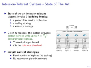
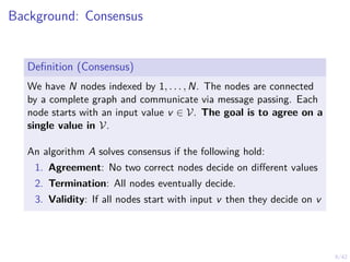
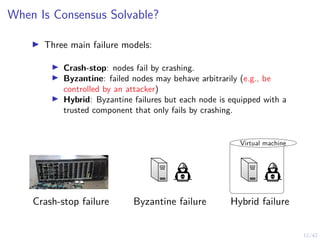
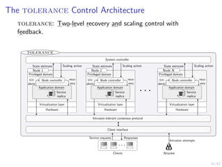
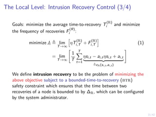
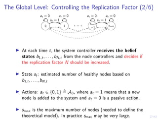
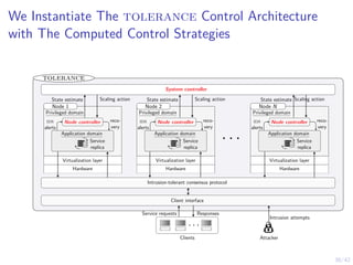
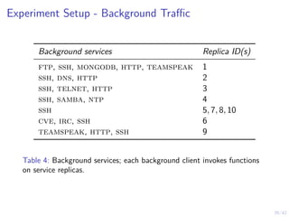
The Local Level: Intrusion Recovery Control (1/4)
▶ Nodes Nt ≜ {1, 2, . . . , Nt} and controllers
π1,t, π2,t, . . . , πN,t.
▶ Hidden states SN = {H, C, ∅} (see
figure).
▶ Actions: (W)ait and (R)ecover
▶ Observation oi,t ∼ Z represents the
number of ids alerts related to node i at
time t.
▶ A node controller computes
bi,t ≜ P[Si,t = C | oi,1, . . .] and makes
decisions ai,t = πi,t(bi,t) ∈ {W, R}.
H C
∅
Crashed
Healthy Compromised
pC1 pC2
pR or a = R
pA](https://image.slidesharecdn.com/nseseminar10nov2023kim-231110114714-7dba48f7/85/Intrusion-Tolerance-for-Networked-Systems-through-Two-level-Feedback-Control-29-320.jpg)
![20/42
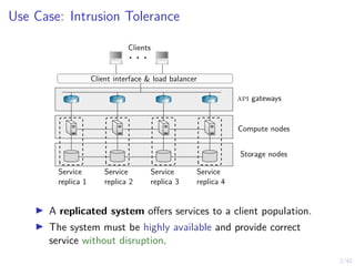
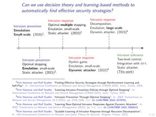
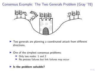
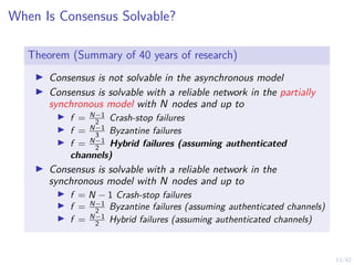
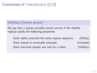
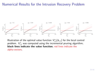
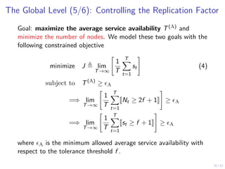
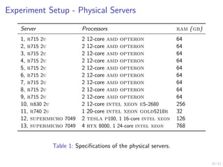
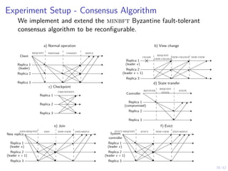
The Local Level: Probability of Failure (2/4)
10 20 30 40 50 60 70 80 90 100
0.5
1
pA = 0.1 pA = 0.05 pA = 0.025
pA = 0.01 pA = 0.005
t
P[St = C ∪ St = ∅]
Probability of node compromise (St = C) or crash (St = ∅) in function of
time t, assuming no recoveries.](https://image.slidesharecdn.com/nseseminar10nov2023kim-231110114714-7dba48f7/85/Intrusion-Tolerance-for-Networked-Systems-through-Two-level-Feedback-Control-30-320.jpg)
![22/42
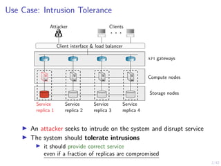
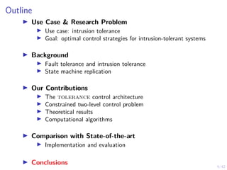
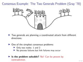
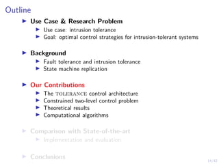
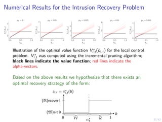
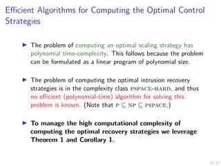
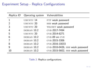
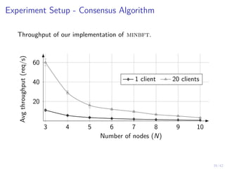
The Local Level: Intrusion Recovery Control (4/4)
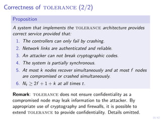
Problem (Optimal Intrusion Recovery Control)
minimize
πi,t ∈ΠN
Eπi,t [Ji | Bi,1 = pA] ∀i ∈ N (2a)
subject to ai,k∆R
= R ∀i, k (2b)
si,t+1 ∼ fN(· | si,t, ai,t) ∀i, t (2c)
oi,t+1 ∼ Z(· | si,t) ∀i, t (2d)
ai,t+1 ∼ πi,t(bi,t) ∀i, t (2e)
ai,t ∈ AN, si,t ∈ SN, oit, ∈ O ∀i, t (2f)](https://image.slidesharecdn.com/nseseminar10nov2023kim-231110114714-7dba48f7/85/Intrusion-Tolerance-for-Networked-Systems-through-Two-level-Feedback-Control-32-320.jpg)
![24/42
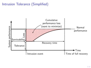
Structure of an Optimal Intrusion Recovery Strategy (1/2)
Theorem (Optimal Threshold Recovery Strategies)
If the following holds
pA, pU, pC1 , pC2 ∈ (0, 1) (A)
pA + pU ≤ 1 (B)
pC1 (pU − 1)
pA(pC1 − 1) + pC1 (pU − 1)
≤ pC2 (C)
Z(oi,t | si,t) > 0 ∀oi,t, si,t (D)
Z is tp-2 (E)
then there exists an optimal recovery strategy π⋆
i,t for each node
i ∈ N that satisfies
π⋆
i,t(bi,t) = R ⇐⇒ bi,t ≥ α⋆
t ∀t, α⋆
t ∈ [0, 1] (3)](https://image.slidesharecdn.com/nseseminar10nov2023kim-231110114714-7dba48f7/85/Intrusion-Tolerance-for-Networked-Systems-through-Two-level-Feedback-Control-35-320.jpg)
![25/42
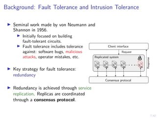
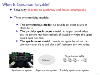
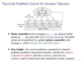
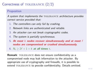
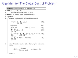
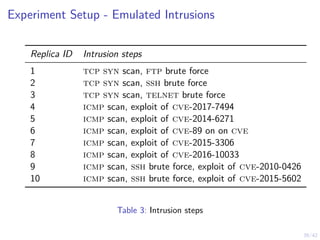
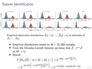
Structure of an Optimal Intrusion Recovery Strategy (2/2)
Corollary (Stationary Optimal Strategy as ∆R → ∞)
The recovery thresholds satisfy α⋆
t+1 ≥ α⋆
t for all
t ∈ [k∆R, (k + 1)∆R] and as ∆R → ∞, the thresholds converge to
a time-independent threshold α⋆.
20 40 60 80 100
0.85
0.9
0.95
α⋆
t
t
The thresholds were computed using the Incremental Pruning algorithm.](https://image.slidesharecdn.com/nseseminar10nov2023kim-231110114714-7dba48f7/85/Intrusion-Tolerance-for-Networked-Systems-through-Two-level-Feedback-Control-36-320.jpg)
![28/42
The Global Level (3/6): Mean Time to Failure
10 20 30 40 50 60 70 80 90 100
200
400
600
pA = 0.1 pA = 0.05 pA = 0.025
pA = 0.01 pA = 0.005
N1
E[T(f )]
Mean time to failure (mttf) in function of the initial number of nodes
N1; T(f )
is a random variable representing the time when Nt < f + 1 with
f = 3 and k = 1; the curves relate to different intrusion probabilities pA.](https://image.slidesharecdn.com/nseseminar10nov2023kim-231110114714-7dba48f7/85/Intrusion-Tolerance-for-Networked-Systems-through-Two-level-Feedback-Control-39-320.jpg)
![29/42
The Global Level (4/6): Reliability Curve
10 20 30 40 50 60 70 80 90 100
0.2
0.4
0.6
0.8
1
N1 = 25 N1 = 50 N1 = 100
N1 = 200 N1 = 400
t
R(t)
Reliability curves for varying number of nodes N; The reliability function
is defined as R(t) ≜ P[T(f )
> t] where T(f )
is a random variable
representing the time when Nt < f + 1 with f = 3.](https://image.slidesharecdn.com/nseseminar10nov2023kim-231110114714-7dba48f7/85/Intrusion-Tolerance-for-Networked-Systems-through-Two-level-Feedback-Control-40-320.jpg)
![31/42
The Global Level (6/6): Controlling the Replication Factor
Problem (Optimal Control of the Replication Factor)
minimize
π∈ΠS
Eπ [J | S1 = N] (5a)
subject to Eπ
h
T(A)
i
≥ ϵA ∀t (5b)
st+1 = fS(st, at, δt) ∈ SS ∀t (5c)
δt ∼ p∆(st) ∀t (5d)
at+1 ∼ πt(st) ∈ AS ∀t (5e)](https://image.slidesharecdn.com/nseseminar10nov2023kim-231110114714-7dba48f7/85/Intrusion-Tolerance-for-Networked-Systems-through-Two-level-Feedback-Control-42-320.jpg)
![32/42
Structure of an Optimal Scaling Strategy
Theorem
If the following holds
∃π ∈ ΠS such that Eπ
h
T(A)
i
≥ ϵA (A)
fS(s′
| s, a) > 0 ∀s′
, s, a (B)
smax
X
s′=s
fS(s′
| ŝ + 1, a) ≥
smax
X
s′=s
fS(s′
| ŝ, a) ∀s, ŝ, a (C)
then there exists two strategies πλ1 and πλ1 that satisfy
πλ1 (st) = 1 ⇐⇒ st ≤ β1 πλ2 (st) = 1 ⇐⇒ st ≤ β2 ∀t (6)
and an optimal randomized threshold strategy π⋆ that satisfies
π⋆
(st) = κπλ1 (st) + (1 − κ)πλ2 (st) ∀t (7)
for some probability κ ∈ [0, 1].](https://image.slidesharecdn.com/nseseminar10nov2023kim-231110114714-7dba48f7/85/Intrusion-Tolerance-for-Networked-Systems-through-Two-level-Feedback-Control-43-320.jpg)
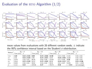
![33/42
Algorithm for The Local Control Problem
Algorithm 1: Recovery Threshold Optimization (rto)
1 Input: η, pA, pC1 , pC2 , pU, Z, ∆R
2 Parametric optimization algorithm: PO
3 Output: A near-optimal local control strategy π̂θ,t
4 Algorithm
5 d ← 1 − ∆R if ∆R < ∞ else d ← 1
6 Θ ← [0, 1]d
7 For each θ ∈ Θ, define πi,θ(bt) as
πi,θ(bt) ≜
(
R if bt ≥ θi where i = max[t, d]
W otherwise
8 Jθ ← Eπi,θ
[Ji ]
9 π̂θ,t ← PO(Θ, Jθ)
10 return π̂θ,t](https://image.slidesharecdn.com/nseseminar10nov2023kim-231110114714-7dba48f7/85/Intrusion-Tolerance-for-Networked-Systems-through-Two-level-Feedback-Control-45-320.jpg)
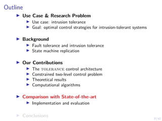

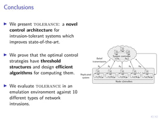

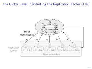
This document outlines a two-level feedback control architecture for intrusion tolerance in networked systems. At the local level, node controllers monitor individual replicas and make recovery decisions based on belief states about their health. At the global level, a system controller scales the replication factor based on belief state information from the node controllers. The architecture provides correct service if certain conditions are met, including maintaining a sufficient number of replicas. The two-level approach models intrusion tolerance as classical machine replacement and inventory replenishment control problems.