1. JohnMichael Croft
File:198045bd-7f35-44c2-808e-eb0aa000a4bb-150213005029-conversion-gate01 Page 1 of 6 John Mic
Part 3:
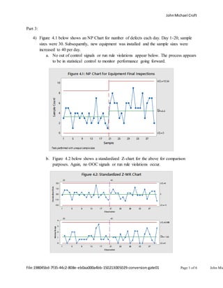
4) Figure 4.1 below shows an NP Chart for number of defects each day. Day 1-20, sample
sizes were 30. Subsequently, new equipment was installed and the sample sizes were
increased to 40 per day.
a. No out of control signals or run rule violations appear below. The process appears
to be in statistical control to monitor performance going forward.
b. Figure 4.2 below shows a standardized Z-chart for the above for comparison
purposes. Again, no OOC signals or run rule violations occur.
2. JohnMichael Croft
File:198045bd-7f35-44c2-808e-eb0aa000a4bb-150213005029-conversion-gate01 Page 2 of 6 John Mic
c. Figure 4.3 below shows an NP Chart by stages (old and new equipment). Again
no OOC signals or run rule violations occur. Notice the newer equipment has a
wider variance due to lack of use suggesting it may need to be monitored and
calibrated to reduce the variance of defects per day.
5) Below are a series of evaluations on the X5 variable assuming the first 30 subgroups as a
baseline with very good control of the process.
a. Figure 5.1 below shows an IMR chart of the first 30 subgroups to estimate the
mean and standard deviation.
2825221 91 61 31 0741
70
65
60
55
50
Observation
IndividualValue
_
X=60.21
UCL=72.62
LCL=47.81
2825221 91 61 31 0741
1 6
1 2
8
4
0
Observation
MovingRange
__
MR=4.66
UCL=15.24
LCL=0
Figure 5.1: IM-R of Subgroups 1-30
3. JohnMichael Croft
File:198045bd-7f35-44c2-808e-eb0aa000a4bb-150213005029-conversion-gate01 Page 3 of 6 John Mic
𝑃𝑟𝑜𝑐𝑒𝑠𝑠 𝑀𝑒𝑎𝑛 = 60.21
𝑃𝑟𝑜𝑐𝑒𝑠𝑠 𝑆𝑡𝑎𝑛𝑑𝑎𝑟𝑑 𝐷𝑒𝑣𝑖𝑎𝑡𝑖𝑜𝑛 =
4.66
1.128
= 4.13
b. Figure 5.2 below attempts to monitor the remaining subgroups based on the
parameter estimates from the first 30 subgroups using an IMR chart. Notice
several OOC and run rule violations in the MR chart that need to be addressed
prior to making meaningful decisions based on the I chart. However, the I chart
displays one OOC and 2 run rule violations.
c. Figure 5.3 simulates the above again, but with a EWMA chart. Again, notice
several OOC points beyond the UCL suggesting the process is unstable and needs
to be calibrated to remove the unwanted variability.
5. JohnMichael Croft
File:198045bd-7f35-44c2-808e-eb0aa000a4bb-150213005029-conversion-gate01 Page 5 of 6 John Mic
i. Subgroups 1-30 represent a stab process with a mean, 60.21 and standard
deviation, 4.13.
ii. Figures 5.2 – 5.4 all suggest assignable cause variation or possible mean
shifts while monitoring subgroups 31-60.
iii. Figure 5.2 suggest an OOC signal at subgroup 46 and run rule violations at
48 and 50.
iv. Figure 5.3 show several OOC signals within the cluster of subgroups 45 –
54 suggesting the process lost control between 31 and 43.
v. Figure 5.4 show several OOC signals from 46 – 57.
vi. Recommend eliminating assignable cause variation and closely
monitoring to reduce variability within the process.
6) Below are several charts evaluating two parameters, separately and together, monitoring
process performance in a multivariate setting.
a. Figures 6.1 and 6.2 below show X6A and X6B to be independently in statistical
control with no OOC signals or run rule violations.
2825221 91 61 31 0741
40
35
30
25
20
Observation
IndividualValue
_
X=29.65
UCL=42.38
LCL=16.93
2825221 91 61 31 0741
1 6
1 2
8
4
0
Observation
MovingRange
__
MR=4.78
UCL=15.63
LCL=0
Figure 6.1: IM-R X6A
6. JohnMichael Croft
File:198045bd-7f35-44c2-808e-eb0aa000a4bb-150213005029-conversion-gate01 Page 6 of 6 John Mic
b. Figure 6.3 performs a multivariate T^2 Chart considering both variables together.
Subgroup 30 appears to be OOC as it exceeds the UCL on the T^2n chart. This
appears consistent with the spike in the Generalized Variance.
c. Considering the interaction of the two effect together allows for OOC signals to
be detected where univariate charts might not.
2825221 91 61 31 0741
25.0
22.5
20.0
1 7.5
1 5.0
Observation
IndividualValue
_
X=20.16
UCL=26.50
LCL=13.82
2825221 91 61 31 0741
8
6
4
2
0
Observation
MovingRange
__
MR=2.384
UCL=7.790
LCL=0
Figure 6.2: IM-R X6B
2825221 91 61 31 0741
20
1 5
1 0
5
0
Sample
Tsquared
Median=2.25
UCL=14.31
2825221 91 61 31 0741
1 .6
1 .2
0.8
0.4
0.0
Sample
GeneralizedVariance
|S|=0.442
UCL=1.443
LCL=0
Figure 6.3: Multivariate Chart