
Recommended
More Related Content
What's hot
What's hot (20)
Similar to Time series project report report
Similar to Time series project report report (20)
Recently uploaded
Recently uploaded (20)
Time series project report report
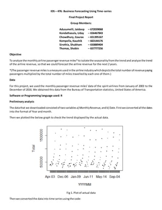
- 1. IDS – 476: Business Forecasting Using Time-series Final Project Report Group Members: Adusumelli, Jaideep – 672039068 Kondathasula, Uday – 656467843 Chowdhury, Gaurav – 651395167 Kompella, Kaushik – 663144176 Sirothia, Shubham – 650889404 Thomas, Shobin – 657777256 Objective To analyze the monthlyairline passengerrevenue miles*toisolate the seasonalityfromthe trendand analyze the trend of the airline revenue, so that we could forecast the airline revenue for the next 2 years. *(The passengerrevenue milesisameasure usedinthe airlineindustrywhichdepictsthe total numberof revenuepaying passengers multiplied by the total number of miles travelled by each one of them.) Data For this project, we used the monthly passenger revenue miles’ data of the spirit airlines from January of 2003 to the December of 2016. We obtained this data from the Bureau of Transportation statistics, United States of America. Software or Programming language used: R Preliminary analysis The datathat we downloadedconsistedof twovariablesa) MonthlyRevenue,andb) Date.Firstweconvertedallthe dates into the format of Year and month. Then we plotted the below graph to check the trend displayed by the actual data. Fig 1. Plot of actual data Thenwe convertedthe datainto time seriesusingthe code:
- 2. > rpm = read.csv("data.csv") > rpm.ts = ts(as.numeric(rpm$Total), start=c(2003,01),freq=12) > plot(rpm.ts,ylab="Total") Fig 2. Time series plot of data Decompositionofdata We thendecomposedthe datainto3 parts a) Trend,b) Seasonality,andc) random. Fig 3. Decomposed graphs of time series data
- 3. As we can see in figure two that our data had an upward increasing trend, hence we had to use the multiplicative decomposition. Xt = Mt * St * Ztj Mt: Trend in the data St: Seasonality in the data Zt: Randomness in the data Thenwe plottedthe autodecompositionfactorgraphfor the decomposeddata. > rpm.acf=acf(as.numeric(Rpm.decom$random), na.action = na.omit, lag.max = 40) Fig 4. ACF plot for the random variable in decomposed data. As we can see thatthe ACFplotshowedveryunevenplot,withnosignificanttrends.Hence,furthermodellingneeded to be done. Thenwe fittedalinearmodel alongwitha seasonal parameter. The ACFplotforthe residualsfromthe linearmodel were as follows. Fig 5. ACF plot for the linear model with seasonality.
- 4. The ACF plotdidn’tdie insteadithadwentonto negative side of the graph. So,we triedfittingaSARIMA model.Forthiswe plottedthe PACFandACFcurvesbelow,whichshow usthatthat the AC F plotdiesoff at 1 andPACFalsodiesof at 1, hence the parametersusedbyuswere p=1, q=1, d=1 withseasonalityont he AR(1) model. Fig 6. PACF plot for the SARIMA model. Fig 7. ACF plot for the SARIMA model. Forecasting Afterthe model buildingwe thenapplieditonourdata whichgave usa forecastof the nexttwelve monthsinthe formof a .txt file which is attached along with this document. We got the following graph as out put.
- 5. Fig 8. Forecasting output of the SARIMA model with the dotted line being the output.