Income Determination under two-sector economy

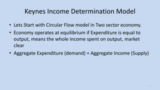
1. Keynes Income Determination Model
• Lets Start with Circular Flow model in Two sector economy.
• Economy operates at equilibrium if Expenditure is equal to
output, means the whole income spent on output, market
clear
• Aggregate Expenditure (demand) = Aggregate Income (Supply)
1

2. The Two Sector Model
(Simple Keynesian Model)
• We start with Circular flow of income in Two Sector Economy,
aggregate expenditure – consumption and investment i.e.
Aggregate Expenditure = C + I
Aggregate Income = C + S
We assume a closed economy (no international trade), no
government
• Saving becomes the only withdrawal and investment the only
injection into the circular flow of income
2

3. Consumption, Saving & Investment
• Consumption spending (C) is household expenditure on
durable and non-durable goods and services while saving (S) is
that part of disposable income not consumed
• Saved income is the one that is borrowed for investment
spending (I)
• Consumption, Saving and Investment play central roles in an
economy
3

4. The Consumption Function
• According to Keynes, Consumption is the function of Income.
In the simple case (this case) the consumption function
relates desired consumption expenditure to disposable
income
4

5. Consumption function Cont’d
• Consumption can be broken down into:
1. Autonomous consumption is the minimal amount consumed by an
individual at zero income (through borrowing or dis-saving)
2. Induced consumption is the one that varies with disposable income
(the higher the income, the higher the amount consumed)
• The consumption function can be represented by the following
equation: C = f (Y) General form
C = Ca + cY Specific form
• Ca represents autonomous and cY represents induced
consumption expenditure 5

6. 6

7. Average Propensity to Consume (APC)
• The average propensity to consume (APC) is the total
consumption spending divided by the total disposable income
APC = C/Y
• APC falls as disposable income increases
• Below break-even APC > 1 (dissaving)
• At break-even APC = 1 (All income consumed)
• Above break-even APC < 1 (saving)
7

8. Marginal Propensity to Consume (MPC)
• The marginal propensity to consume (MPC) is the amount of
extra consumption generated by an extra dollar of disposable
income and is given by the formula:
MPC = ∆C/∆Y = c
• The MPC gives the slope of the C-function and 1 > MPC > 0
for all levels of income
• For every $1 of income, less than $1 is spent on consumption
and the rest is saved
8

9. 9
0
1000
2000
3000
4000
5000
0 1000 2000 3000 4000 5000 6000
Consumption
Income
Consumption Function

10. 10
Disposable
Income YD
45º Line
a
Desired
ConsumptionC
C = Ca + cY
Y1
Y2
Induced
Consumption
Autonomous
Consumption
Consumption function Cont’d

11. The Saving Function
• Saving is all the disposable income that is not spent on
consumption, that is:
S = Y – C
• Inverse of consumption function
• The relationship between desired saving and income is
represented by the saving function shown in the figure below.
S = Sa + sY , Sa = - Ca, and s = - c
11

12. Average Propensity to Save (APS)
• The proportion of disposable income that households want to
save is called the average propensity to save (APS).
• It is derived by dividing the total desired saving by total
disposable income:
APS =
𝑺
𝒀
(=1 – Average Propensity to Consume)
12

13. Y C MPC S MPS
0 600 Change C
/Change Y
-600 Change
S/Change Y
1000 1300 700/1000=
0.7
-300 300/1000 =
0.3
2000 2000 0.7 0 300/1000 =
0.3
3000 2700 0.7 300 0.3
4000 3400 0.7 600 0.3
5000 4100 0.7 900 0.3
13

14. Marginal Propensity to Save (MPS)
• the extra saving generated by an extra dollar of disposable
income is called the marginal propensity to save (MPS).
• The MPS is also the slope of the S-function given by the
formula:
MPS= s =
∆𝑺
∆𝒀
= (1 – MPC = 1-c)
• The saving line cuts the horizontal axis at the break-even level
of income, thus:
S = 0 when C = Y
14

15. Graphical Presentation of the
S-function
0
DesiredSavingS
S = -a + (1-b)Y
-a
Disposable Income YD
15
)1( c
Y
S
Slope 



ΔY
ΔS

16. Consumption Function & The 45⁰ Line
• In order to understand Consumption and Equilibrium output in
economy, we draw a 45⁰ line in the graph.
• This line shows: Y = C + S
• Income is Either consumed or saved.
16

17. Consumption function & the 450 Line
Disposable Income YD
45º
Y = C + S
a
DesiredConsumptionC
C = Ca + cY
Saving ( Y > C)
Dissaving ( Y < C)
17

18. 18
Disposable
Income Y
45º Line
C1
a
Desired
ConsumptionC
C2
Y1
Y2
ΔC
ΔY
b
Y
C
YY
CC
Slope 






12
12
Induced
Consumption
Autonomous
Consumption
Output or Income
Consumption function Cont’d
C = Ca + cY

19. Consumption & Saving Relation
The saving function is
basically the vertical
distance between the
consumption function
and the 450 line since
disposable income must
either be consumed or
saved. When C exceeds
income, S<0, when C is
below income, S>0.
19
(i)Consumption function
C = a + bY
S = -a + (1-b)Y
Disposable Income (Y)
450 Line
a
Ye
0
0
-a
Disposable Income (Y)
450 Y = C + S
(ii) Saving function
Ye

20. Investment Spending
• Three components of investment spending are:
a) Inventory accumulation (finished goods, work in progress and raw
materials)
b) Residential housing and construction
c) Business fixed capital formation
• All these components are negatively related to interest rates
20

21. Investment and Income Diagram
21
Real GDP (Y)
Investment(I)
I = I0I0
0
Investment is not dependent on income, it does not change with
income

22. Back to: Two-Sector Model of Income Determination
• Initially we said desired aggregate spending is:
AE = C + I
= (Ca + cY) + I0
• Thus the AE function is a summation of the consumption
function and autonomous investment spending as shown
below:
22

23. Aggregate Expenditure Function
23
Real GDP (Y)
DesiredSpending(AE)
AE = C + I
I = I0
a
a + I0
The AE function is parallel to the consumption function, the
vertical distance between them being equal to the autonomous
investment I0
C = Ca + cY

24. • Given that consumption has an autonomous
and induced component, the constant
investment (I0) adds to the autonomous
component of consumption (a) hence the
intercept becomes (a + I0)
• Superimposition of a 45o line (a locus of all
points where AE=Y) which shows all possible
equilibrium points will help us determine the
equilibrium level of output
24
AE Function Cont’d

25. AE Function & 45o Line
25
45º
AE = Y
Real GDP (Y)Ye
DesiredSpending(AE)
AE = C + I
AEe
AE > Y
AE < Y

26. 26
1. AE > Y – Excess Demand – unexpected
decrease in inventories – planned output rises
2. AE < Y – Excess Supply – unexpected increase
in inventories – planned output decreases
3. Equilibrium level of GDP is determined where
AE = Y i.e. where AE curve intersects the 45o
line
AE Function & 45o Line Cont’d

27. Saving & Investment Approach
• Equilibrium output can be determined where planned
saving (S) is equal to planned investment spending
S = I
• Saving is a leakage (withdrawal) and Investment is an
injection (addition). Income and spending can only be in
equilibrium if leakages equal injections
• The intersection of the saving and investment functions at
point E in diagram (b) gives equilibrium income Ye
27

28. I & S Approach for Equilibrium in Economy
28
0
Desired(I&S)
S = -Ca + (1-c)Y
-a
Real GDP (Y)
I0
Ye

29. 29
Equilibrium in Economy

30. • At GDP level Ye, S = I (b), hence Y = AE in (a) thus
the economy is at equilibrium
• At GDP levels above Ye, S > I (b) (households saving
more than firms want to invest hence demand will
be low), hence AE < Y in (a) thus firms cut down
output and GDP declines towards Ye
• At GDP levels below Ye, S < I (b) households saving
less than firms want to invest hence demand will
be high, hence AE > Y in (a) thus firms increase
output and GDP rises towards Ye
30

31. 31

32. Keynesian Equilibrium with Government and the Foreign Sector
Added (cont'd)
• Determining the equilibrium level of GDP per year
– We are now in a position to determine the equilibrium level of real
GDP per year
– Remember that equilibrium always occurs when total planned real
expenditures equal real GDP