1. A New Selection Criteria for Red and Obscured Quasars in Stripe 82
Milena Crnogorˇcevi´c, Middlebury College
Henry Daniels-Koch, Bowdoin College
Advisor: Eilat Glikman, Middlebury College
Abstract
Most massive galaxies have supermassive black holes at their centers. In order to thor-
oughly understand galaxy evolution, we study the evolution of their corresponding supermas-
sive black holes. Supermassive black holes' gravitational potential pulls in and excites the
gas in their vicinities, causing the gas to emit radiation that we detect as quasars. By study-
ing the evolution of a quasar we indirectly learn about the evolution of the black hole at its
center which can give us some insight into the evolution of the galaxy itself. Our research
concerns the ”teenage years” of quasars which are obscured by dust. Newly formed quasars
often have dust particles around them that absorb and scatter some of the blue light emitted,
effectively ”reddening” the image of the quasar. In our research we utilize a new selection cri-
teria for dust-reddened quasars by studying objects in the infrared region. We consider heavily
obscured, but luminous quasars using infrared selection from Wide-field Infrared Survey Ex-
plorer (WISE). After obtaining data from NASA's infrared telescope (IRTF), we generate an
emission spectrum for each quasar, calculate redshifts, use Gaussian fitting to approximate
fluxes of emission peaks, and plot BPT diagrams. We determine from our BPT diagrams that
6 out of the 8 sources we select are quasars using new selection techniques.
Introduction
As two or more galaxies merge to create one massive galaxy, their black holes combine into
a single black hole. These mergers are followed by a period of intense star formation. At the
same time large amounts of gas are funneled to the bottom of the new gravitational potential.
Supermassive black holes actively accrete gas from their surroundings to form accretion disks,
the defining characteristic of Active Galactic Nuclei (AGN). Quasars are the most luminous type
of AGN. The accretion in a quasar, which emits radiation at nearly all wavelengths, excites the
surrounding atomic gas. However, gas particles surrounding a newly formed quasar absorb and
scatter a significant amount of the blue light emitted by that quasar. This results in a decrease of
the observed luminosity and the ”reddening” of the source in the optical region.
Gases accrete onto a black hole from the accretion disc. Radiation from the quasar can be
emitted by fast moving clouds causing broad line emissions or by slower moving clouds causing
narrow line emissions. Dust around the quasar absorbs blue light, reddening the image of the
quasar. Dust-reddened quasars with lower luminosities are difficult to detect, hence it is important
to come up with a good selection criteria. In the late 1950s, it was initially thought all quasars emit
light in only the radio region of the electromagnetic spectrum, allowing them to be easily identified
by radio telescopes. However, (Kellermann et al., 1989) showed that only about 10% of all quasars
emit in the radio region, necessitating a revision in the quasar selection criteria . In the 2000s, the
Sloan Digital Sky Survey (SDSS) began mapping sections of the sky in the optical region to create
a large database of quasars.
1

2. Our understanding of quasars was revolutionized again with the realization that a significant
portion of the quasar population is dust-reddened and missing from optical quasar surveys such
as the Sloan Digital Sky Survey (SDSS). In its selection process, SDSS makes use of the fact
that most quasars emit more light in the blue region than in the red region of the optical spectra.
However, when quasars are dust-reddened, SDSS's selection algorithm cannot detect them due to
their decreased observed brightness and colors that resemble galaxies and stars. This is problematic
for studying the overall quasar population because a significant group of quasars are missing from
SDSS's quasar population.
To gain a more representative observational data set of quasars and therefore supermassive black-
holes, we must add the significant population of dust-reddened quasars. Until recently, it was not
possible to reliably select a comprehensive set of dust reddened quasars. (Glikman et al., 2007,
Glikman et al., 2012) took the first step by showing that about 20% of all radio-loud quasars are
dust-reddened. However, it remains unknown if radio-quiet, dust-reddened quasars also constitute
20% of radio-quiet quasars. In order to decouple dust-reddened quasars and radio loud quasars,
we need to utilize methods of selecting radio-quiet, but dust-reddened quasars.
Selection Process
Using recently released infrared data from the Wide Field Infrared Survey Explorer (WISE), we
utilize new selection techniques from (Lacy et al., 2004, Lacy et al., 2007) and (Stern et al., 2005).
(Lacy et al., 2004, Lacy et al., 2007) and (Stern et al., 2005) found radio-loud, dust-reddened
quasars through a radio selection process, but then studied their selection's infrared properties.
(Lacy et al., 2004, Lacy et al., 2007) and (Stern et al., 2005) suggest infrared selection criteria for
detecting dust-reddened quasars. We apply (Lacy et al., 2004, Lacy et al., 2007) and (Stern et al.,
2005)'s infrared selection criteria to find radio-quiet, dust-reddened quasars.
We begin our selection method by finding objects from the WISE database in Stripe 82, a well-
studied region of sky. We choose only the objects that are brighter than 6.6mag. Using the infrared
selection criteria from (Lacy et al., 2004, Lacy et al., 2007) and (Stern et al., 2005) we filter out
objects that do not satisfy color-to-color ratios as seen in Figure 1. Using the Sloan Digital Sky
Survey (SDSS), we match our objects from WISE to the objects in SDSS's database. When SDSS
identifies a quasar candidate, it obtains a spectrum for that quasar. However, SDSS's selection al-
gorithm cannot identify dust-reddened quasars and therefore does not have spectra for them. Thus,
we select objects in the matched list that do not contain spectra in SDSS in order to identify candi-
dates for dust-reddened quasars. We further narrow our subset to only the most luminous objects
in the infrared (luminosity of K < 15.1), arriving at a list of 48 objects. Lastly, we remove artifacts
by visual inspection. We notice that the density of luminous objects on the edge of Stripe-82 is
significantly higher from the rest of the area, hence conclude that these objects are pseudo-sources
and appear in our images as a result of the limitation of the electronics used. After examining
images of these objects in the SDSS database, we arrive at a final list of 12 potential dust-reddened
quasars. This process is shown in the selection criteria flow chart (Figure 2).
2

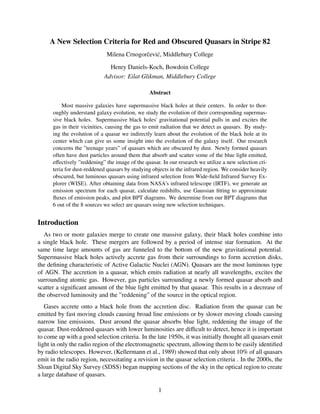
3. Fig. 1.— (Wright et al., 2010). Color-to-color ratios of astrophysical objects with infrared emissions. The
dots shown are the QSO objects with WISE colors of previously selected radio-loud, dust reddened quasars.
Our selection criteria for radio-quiet, reddened quasars is based on color to color of QSO region shown.
WISE Database
563 million objects
Select WISE objects in Stripe 82
-50 < RA < 59, -1.25 < DEC < 1.25
Select brightest objects in WISE
3437 objects
Select objects with color-to-color
ratios characteristic of a quasar
1067 objects
Select brightest objects in
2MASS
192 objects
Select brightest objects in
red region in SDSS
614 objects
Select objects with no existing spetra
48 objects
Remove artifacts by visual inspection
12 objects
Fig. 2.— Quasar Selection Process Flow Chart. Utilizes criteria from WISE, 2MASS, and SDSS to select
objects that are bright, have color-to-color ratios indicative of quasars, and do not contain spectra in SDSS.
3

4. Data Reduction
The optical data used in this research is obtained from the optical telescope at Keck Observatory,
and the infrared observations are conducted via NASA's SpeX telescope. The reduction process
of the optical images consists of removing any additive effects by subtracting the overscan region
and the combined bias, and of removing any multiplicative effects by dividing by the combined
flat-field.
The first step in CCD reduction process is removing the overscan. Overscan is the region that is
added to the frame thereafter and is used to minimize errors that arise from telescope's changeable
physical characteristics, such as its position, temperature, etc. Thirty two pixels at the right edge
are defined to be the overscan region, which values are averaged and subtracted from each frame.
The next step consists of subtracting the combined bias from each image. Bias frames are
images taken by a telescope without the light exposure in a short integration time that allow us to
approximate the additive effects of an individual pixel due to the instrument’s previous use. Ten
biases are combined into a single bias in PyRAF and the combined bias is then subtracted from all
the images.
Final step in CCD Reduction is dividing the images by the combined flat-field. Flat-field image
is a short exposure image of the white screen that is shone upon by a uniform light source and is
used to account for the differences between pixels due their different quantum efficiencies. After
combining ten flats and normalizing the resulting image, we divide objects' images by the com-
bined flat-field. The spectra are extracted and the sky is removed from each frame. The fluxes
are then calibrated by using the sensitivity function and normalized. Then the known wavelengths
from spectra of Argon and Neon are matched to the pixels along the dispersion axis to determine
the wavelength solution.
Finally, the infrared data is combined with the corresponding optical spectra reduced in PyRAF
to produce higher-range wavelength spectra, some of which are shown in Figure 3.
Redshift Calculation and Gaussian Fitting
The light from the objects we observed takes between 1 and 8 billion light years to travel from
the source to the observer, depending on their distance. While the light is traveling to Earth,
the expansion of the universe causes a redshift in the emitted wavelengths. Thus, emission lines
corresponding to certain gases coming from these sources will be shifted to higher wavelengths
compared to the emission lines recorded in a laboratory. In PyRAF, we identify wavelengths of
peaks in various emission spectra and match them to the wavelengths of emissions from gases
found in a laboratory. We calculate the redshift z by using the following expression:
1 + z =
λobs
λemit
,
where λobs is the observed wavelength of emission line from quasar, and λemit is the emitted
wavelength observed in a laboratory. Table 1 lists all the redshifts found and Figure 3 shows a plot
of six emission spectra with their corresponding redshifts. Next, we determine fluxes by fitting
Gaussian curves to emission spectra in IDL. An example of such fitting is shown in Figure 4.
4

5. Fig. 3.— Combined optical and infrared spectra of 6 quasar candidates. Peaks correspond to emissions by
gases around the quasar. By matching peaks in the spectra with emission wavelengths in labs on Earth, we
calculate redshifts.
Fig. 4.— Gaussian Fits. We fit Gaussian curves to peaks in order to find the total flux emitted by a specific
gas. Fluxes were used to create BPT diagrams.
5

6. BPT Diagrams
BPT diagrams are used to classify extragalactic objects based on various emission-line intensity
ratios according to the principal excitation mechanism. As a result of such categorization, most
extragalactic objects can be placed in one of the four categories: (a) photoionized by O or B stars,
high energy sources emitting mostly in the UV region of the emission spectra, (b) photoionized
by a power-law continuum sources with spectral energy distribution that is proportional to the
frequency of the emitted radiation, (c) shock-wave heating, or (d) planetary-nebulae, photoionized
by stars that are usually much hotter than the galactic O-stars. The boundaries between the high
energy objects and low energy objects, K-lines, are determined by (Kewley et al., 2006). We
utilize this categorization from (Baldwin et al., 1981) and by using the fluxes found from fitting
the Gaussian curves we calculate the results shown in Figure 5.
Object Redshift log(O(I I I)
H β ) log( N (I I)
Hα ) log( S(I I)
Hα ) log(O(I)
Hα ) Type (I) Type (II) Type (III)
2152 0.582 -0.73 -1.38 -2.48 NaN starb starb AGN
2057 0.332 1.03 -0.60 NaN -0.13 AGN AGN AGN
2355 0.322 0.35 -0.69 -0.98 -1.86 starb starb starb
0103 0.268 1.12 NaN NaN NaN - - -
2054 0.203 0.73 -0.12 -0.13 -0.57 AGN AGN AGN
0306 0.189 1.75 -0.63 -0.47 0.78 AGN AGN AGN
2252 0.167 0.17 -0.19 -0.33 -0.68 starb starb starb
2246 0.122 0.30 -0.10 -0.48 -1.33 AGN starb starb
0349 0.109 1.41 0.02 -0.37 -0.87 AGN AGN AGN
Table 1: Numerical values of the corresponding redshifts and ratios necessary for the BPT diagrams. We
conclude that 6 out of 9 objects are quasars.
Fig. 5.— BPT Diagrams. We found flux ratios of O(I I I)
H β , N (I I)
Hα , S(I I)
Hα , and O(I)
Hα . BPT diagram shows that
objects with high luminosities (above and to the right of the lines shown) are quasars. We conclude that 5
out of 8 plottable objects are quasars.
6

7. Conclusion
In combination with the X-ray observations, our sample of luminous obscured quasars is pro-
viding, for the first time, a chance to study the most extreme quasars that have been missed by
traditional quasar selection methods. This small sample of low redshift, yet very luminous, ob-
scured quasars is an ideal sample for follow up studies with high resolution imaging by the Hubble
Space Telescope. Follow up studies will look for direct evidence of mergers as has been done
for the radio-selected red quasars at higher redshifts. High resolution imaging in sub-milimeter
wavelengths with the ALMA telescope array in Chile will allow us to study their molecular gas
content, which will give us a more complete picture of how quasars transition from obscured to
unobscured, especially when they are the result of a galaxy merger.
Our sincere thanks goes to Professor Eilat Glikman for her precious support and guidance and
great ability to impart knowledge and passion for our universe. We thank Jonathan Kemp for
his immense help with coding and for teaching us about telescopes. We gratefully acknowledge
the National Science Foundation's support of the Keck Northeast Astronomy Consortium's REU
program. This research has made use of data from NASA’s IRTF telescope, the WISE database,
SDSS, the Keck Observatory, and NASA’s SpeX telescope. Last, but certainly not least, we thank
the other half of Professor Glikman's lab, Carol Hundal and Larson Lovdal, with whom we spent
the summer discussing the complex nature of our existence.
References
A. Baldwin, M.M. Phillips, R. Terlevich. Classification parameters for the emission-line spectra
of extragalactic objects. 93, 5-19 (1981).
E. Glikman, T. Urrutia, M. Lacy, S. G. Djorgovski, A. Mahabal, A. D. Myers, N. P. Ross, P.
Petitjean, J. Ge, D. P. Schneider, D. G. York. FIRST-2MASS Red Quasars: Transitional Objects
Emerging from the Dust. 757, 51 (2012).
E. Glikman, D. J. Helfand, R. L. White, R. H. Becker, M. D. Gregg, M. Lacy. The FIRST-
2MASS Red Quasar Survey. 667, 673-703 (2007).
K. I. Kellermann, R. Sramek, M. Schmidt, D. B. Shaffer, R. Green. VLA observations of objects
in the Palomar Bright Quasar Survey. 98, 1195-1207 (1989).
L.J. Kewley, B. Groves, G. Kauffmann, T. Heckman. The host galaxies and classification of
active galactic nuclei. 372, 961-976 (2006).
M. Lacy, A. O. Petric, A. Sajina, G. Canalizo, L. J. Storrie-Lombardi, L. Armus, D. Fadda, F. R.
Marleau. Optical Spectroscopy and X-Ray Detections of a Sample of Quasars and Active Galactic
Nuclei Selected in the Mid-Infrared from Two Spitzer Space Telescope Wide-Area Surveys. 133,
186-205 (2007).
M. Lacy, L. J. Storrie-Lombardi, A. Sajina, P. N. Appleton, L. Armus, S. C. Chapman, P. I. Choi,
D. Fadda, F. Fang, D. T. Frayer, I. Heinrichsen, G. Helou, M. Im, F. R. Marleau, F. Masci, D. L.
Shupe, B. T. Soifer, J. Surace, H. I. Teplitz, G. Wilson, L. Yan. Obscured and Unobscured Active
Galactic Nuclei in the Spitzer Space Telescope First Look Survey. 154, 166-169 (2004).
7

8. D. Stern, P. Eisenhardt, V. Gorjian, C. S. Kochanek, N. Caldwell, D. Eisenstein, M. Brodwin,
M. J. I. Brown, R. Cool, A. Dey, P. Green, B. T. Jannuzi, S. S. Murray, M. A. Pahre, S. P. Willner.
Mid-Infrared Selection of Active Galaxies. 631, 163-168 (2005).
E. L. Wright, P. R. M. Eisenhardt, A. K. Mainzer, M. E. Ressler, R. M. Cutri, T. Jarrett, J. D.
Kirkpatrick, D. Padgett, R. S. McMillan, M. Skrutskie, S. A. Stanford, M. Cohen, R. G. Walker, J.
C. Mather, D. Leisawitz, III Gautier, I. McLean, D. Benford, C. J. Lonsdale, A. Blain, B. Mendez,
W. R. Irace, V. Duval, F. Liu, D. Royer, I. Heinrichsen, J. Howard, M. Shannon, M. Kendall, A.
L. Walsh, M. Larsen, J. G. Cardon, S. Schick, M. Schwalm, M. Abid, B. Fabinsky, L. Naes, C.-W.
Tsai. The Wide-field Infrared Survey Explorer (WISE): Mission Description and Initial On-orbit
Performance. 140, 1868-1881 (2010).
8