Bayesian Belief Networks for dummies
•Download as PPTX, PDF•
53 likes•55,977 views

introduction to Bayesian Belief Networks for dummies, or more precisely more for business men rather than for mathematicians

Recommended
Recommended
More Related Content
What's hot
What's hot (20)
Viewers also liked
Viewers also liked (11)
Recently uploaded
Recently uploaded (20)
Bayesian Belief Networks for dummies
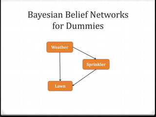
- 1. Bayesian Belief Networks for Dummies Weather Lawn Sprinkler
- 2. Bayesian Belief Networks for Dummies 0 Probabilistic Graphical Model 0 Bayesian Inference
- 3. Bayesian Belief Networks (BBN) BBN is a probabilistic graphical model (PGM) Weather Lawn Sprinkler
- 4. Bayesian Belief Network 0 Graphical (Directed Acyclic Graph) Model 0 Nodes are the features: 0 Each has a set of possible parameters/values/states: 0Weather = {sunny, cloudy, rainy}; Sprinkler = {off, on}; Lawn = {dry, wet} 0BBN sample case: {Weather = rainy, Sprinkler = off, Lawn = wet} 0 Edges / Links represent relations between features 0 Get used to talking in ‘graph language’: 0Lawn is a child of its two parents: Weather and Sprinkler 0 Direction of edges basically indicates Causality: 0Either rainy weather or turning on the sprinkler may cause wet lawn 0 Edges direction from {Weather / Sprinkler} to Lawn Weather Lawn Sprinkler
- 5. BBN – Modeling Reality with Probabilities 1. Each node / feature is a random variable 0 Takes multiple parameters / values / states 0 States occur with a certain probability 0 Example: a fair coin has two possible values: {heads, tails}, each occurs with 50% probability
- 6. BBN – Modeling Reality with Probabilities – cont. 2. We call these probabilities of occurring states - Beliefs 0Example: our belief in the state {coin=‘head’} is 50% 0If we thought the coin was not fair, then our belief for the state {coin=‘head’} wouldn’t be 50% 0 Bayesian Belief Network 3. All beliefs of all possible states of a node are gathered in a single CPT - Conditional Probability Table
- 7. CPT - Conditional Probability Table Weather Lawn Sprinkler Weather (London) Sunny 10% Cloudy 30% Rainy 60% Sprinkler Weather On Off Sunny 20% 80% Cloudy 10% 90% Rainy 0% 100% Lawn Weather Sprinkler Wet Dry Sunny On 20% 80% Cloudy On 40% 60% Rainy On 100% 0% Sunny Off 0% 100% Cloudy Off 10% 90% Rainy Off 100% 0% Weather (Israel) Sunny 70% Cloudy 20% Rainy 10% Prior Probability P(Sprinkler = ‘on’ | weather = ‘sunny’) = 20% Conditional Probability Probability: all beliefs must sum up to 100%
- 8. Bayesian Belief Networks for Dummies 0 Probabilistic Graphical Model 0 Bayesian Inference
- 9. BBN A Probabilistic Graphical Learning Model 0 BBN is a 2-component model: 0 Graph 0 CPTs Weather Lawn Sprinkler Weather (London) Sunny 10% Cloudy 30% Rainy 60% Sprinkler Weather On Off Sunny 20% 80% Cloudy 10% 90% Rainy 0% 100% Lawn Weather Sprinkle r Wet Dry Sunny On 20% 80% Cloudy On 40% 60% Rainy On 100% 0% Sunny Off 0% 100% Cloudy Off 10% 90% Rainy Off 100% 0%
- 10. BBN Machine Learning Process counting {Weather = ‘rainy’ ; Sprinkler = ‘off’’ ; Lawn = ‘wet’} {Weather = ‘sunny’ ; Sprinkler = ‘on’’ ; Lawn = ‘wet’} {Weather = ‘sunny’ ; Sprinkler = ‘off’’ ; Lawn = ‘dry’} {Weather = ‘cloudy’ ; Sprinkler = ‘off’ ; Lawn = ‘dry’} Weather Lawn Sprinkler Weather (London) Sunny 10% Cloudy 30% Rainy 60% Sprinkler Weather On Off Sunny 20% 80% Cloudy 10% 90% Rainy 0% 100% Lawn Weather Sprinkler Wet Dry Sunny On 20% 80% Cloudy On 40% 60% Rainy On 100% 0% Sunny Off 0% 100% Cloudy Off 10% 90% Rainy Off 100% 0% lots of training cases We begin with a model
- 11. BBN – Predicting (Inferencing) 0 Bayesian Inference: After training (CPT calculation), we can then answer questions like: 0 Given a rainy weather, is the lawn wet? 0 Given that the lawn is wet, what could be the reason for that? 0Rainy weather? or 0A turned-on sprinkler? Weather Lawn Sprinkler Stay Tuned! The real action begins... Trivial answer - not interesting Cool
- 12. Bayesian Inference 0 Bayes’ Theorem: 0 Philosophically: Knowledge is power! Thomas Bayes 18th century Newborn is AB- ? P = 1% Our Prior Belief Hypothesis = what we seek
- 13. Bayesian Inference 0 Bayes’ Theorem: 0 Philosophically: Knowledge is power! Thomas Bayes 18th century Newborn is AB- ? P = 1% Our Prior Belief Hypothesis = what we seek Mother is AB- Evidence
- 14. Bayesian Inference 0 Bayes’ Theorem: 0 Philosophically: Knowledge is power! 0 Bayesian Updating: Evidence updates belief Thomas Bayes 18th century Newborn is AB- ? P = 1% Our Prior Belief Hypothesis = what we seek Mother is AB- Evidence P = ? Our a posteriori Updated Belief
- 15. Bayesian Inference 0 Bayes’ Theorem: 0 Philosophically: Knowledge is power! 0 Bayesian Updating: Evidence updates belief Thomas Bayes 18th century Newborn is AB- ? P = 1% Our Prior Belief Hypothesis = what we seek Mother is AB- Evidence P = ? Our a posteriori Updated Belief Remember! Links are directed from what we seek to what we observe
- 16. Bayesian Inference – Belief Propagation 0 Given that the lawn is wet, what could be the reason for that? 0 Rainy weather? or 0 A turned-on sprinkler? Weather Lawn Sprinkler Hypotheses Evidence Prior P(Sprinkler = ‘On’) P(Sprinkler = ‘Off’) Prior P(Weather = ‘Sunny’) P(Weather = ‘Rainy’)
- 17. Bayesian Inference – Belief Propagation 0 Given that the lawn is wet, what could be the reason for that? 0 Rainy weather? or 0 A turned-on sprinkler? Weather Lawn Sprinkler Hypotheses Evidence Prior P(Sprinkler = ‘On’) P(Sprinkler = ‘Off’) Prior P(Weather = ‘Sunny’) P(Weather = ‘Rainy’) A Posteriori P (Sprinkler = ‘On’ | Lawn = ‘wet') P (Sprinkler = ‘Off’ | Lawn = ‘wet') A Posteriori P(Weather = ‘Sunny’ | Lawn = ‘wet') P(Weather = ‘Rainy’ | Lawn = ‘wet')
- 18. MAP = Bayes Decision Rule 0 So what to predict? Rainy weather or turned-on sprinkler? 0 MAP: choose Maximum A posteriori Probability 0 For P(Weather=‘rainy’ | Lawn=‘wet’) = 0.1 ; P(Sprinkler=‘On’ | Lawn=‘wet’) = 0.08 0Choose Weather = ‘rainy’ , i.e. given the lawn is wet it’s more probable that a rainy weather caused it rather than a turned-on sprinkler Weather Lawn Sprinkler Hypotheses Evidence A Posteriori P(Sprinkler = ‘On’ | Lawn = ‘wet') P(Sprinkler = ‘Off’ | Lawn = ‘wet') A Posteriori P(Weather = ‘Sunny’ | Lawn = ‘wet') P(Weather = ‘Rainy’ | Lawn = ‘wet')
- 19. Thank You
- 20. Appendix A BBN – Likelihood Estimation 0 Parameters Estimation = Assigning probabilities to parameters (CPTs’ entries) 0 One method of computing these probabilities is by Likelihood Estimation, using statistics: 0 Tossing a coin for 100 times and getting 040 times {‘head’} 060 times {‘tail’} 0 Is the process of likelihood estimation of {head, tail} parameters: 0The likelihood of ‘head’ parameter is 40% = ‘head’ is 40% likely to happen 0The likelihood of ‘tail’ parameter is 60% = ‘tail’ is 60% likely to happen
- 21. BBN – Likelihood Estimation of CPTs 0 Training: 0We observe the system for 1,000 times 0 {weather=‘cloudy’ ; sprinkler=‘off’ ; lawn=‘wet’} 0 {weather=‘sunny’ ; sprinkler=‘off’ ; lawn=‘dry’} 0 … 0Likelihood Estimation of Belief CPTs = Counting all observations 0e.g. out of 50 observed cases of {weather=‘cloudy’ ; sprinkler=‘off’ ; lawn=*} in 30 of them lawn was dry and in 20 of them it was wet, we then get: 0 P(lawn = ‘wet’ | weather=‘cloudy’ & sprinkler=‘off’) = 20 / 50 = 40% 0 P(lawn = ‘dry’ | weather=‘cloudy’ & sprinkler=‘off’) = 30 / 50 = 60%
- 22. Appendix B The mathematics behind the scenes
- 23. Probabilities – could be fun 0 A model’s goal: approximating the real world as close as possible “A probabilistic model models the real world using probabilities” 0 A probabilistic model’s goal: estimate its underlying joint probability distribution as accurate as possible Weather Sprinkler Lawn Prob Sunny On Wet 20% Sunny On Dry 10% Sunny Off Wet 0% Sunny Off Dry 10% Rainy On Wet 0% Rainy On Dry 0% Rainy Off Wet 60% Rainy Off Dry 0% table of all probabilities of all possible combinations of states in that world model
- 24. BBN - Factorization 0 BBN estimates its global underlying joint probability by factorization: 1. Separately estimating all its belief CPTs 2. Multiplying them P(weather, sprinkler, lawn) = P(weather) x P(sprinkler | weather) x P(lawn | sprinkler, weather) For example: P(weather=‘sunny’, sprinkler=‘on’, lawn=‘wet’) = = P(weather=‘sunny’) x P(sprinkler=‘on’ | weather=‘sunny’) x P(lawn=‘wet’ | sprinkler=‘on’ , weather=‘sunny’) = 0.1 * 0.2 * 0.2 = 0.004 Weather (London) Sunny 10% Cloudy 30% Rainy 60% Sprinkler Weather On Off Sunny 20% 80% Cloudy 10% 90% Rainy 0% 100% Lawn Weather Sprinkler Wet Dry Sunny On 20% 80% Cloudy On 40% 60% Rainy On 100% 0% Sunny Off 0% 100% Cloudy Off 10% 90% Rainy Off 100% 0%
- 25. 0 BBN estimates its global underlying joint probability by factorization: 1. Separately estimating all its belief CPTs 2. Multiplying them: P(weather, sprinkler, lawn) = P(weather) x P(sprinkler | weather) x P(lawn | sprinkler, weather) This should be your expression now. Wonder why? The answer is just one slide ahead BBN - Factorization
- 26. P(weather, sprinkler, lawn) = P(weather) x P(sprinkler | weather) x P(lawn | sprinkler, weather) 0 Why is it so fascinating? It’s the basic chain rule from first course in probability: 0P(A,B,C…) = P(A) x P(B|A) x P(C|A,B) x …. 0 That’s the beauty! By simply estimating the independent CPTs, BBN estimates very complex networks! CPTs BBN - Factorization
- 27. Curse of Dimensionality Reason #2 for being happy 0 Network Size = number of parameters Weather Sunny Rainy Weather Sunny Rainy
- 28. Curse of Dimensionality Reason #2 for being happy 0 Network Size = number of parameters Weather Sprinkler Sunny Rainy On Off weather sprinkler Sunny On Sunny Off Rainy On Rainy Off Weather Sunny Rainy
- 29. Curse of Dimensionality Reason #2 for being happy 0 Network Size = number of parameters Weather Lawn Sprinkler Sunny Rainy On Off Wet Dry weather sprinkler Sunny On Sunny Off Rainy On Rainy Off Weather Sprinkler Lawn Sunny On Wet Sunny On Dry Sunny Off Wet Sunny Off Dry Rainy On Wet Rainy On Dry Rainy Off Wet Rainy Off Dry Weather Sunny Rainy
- 30. Curse of Dimensionality Reason #2 for being happy 0 Network Size = number of parameters Weather Lawn Sprinkler Sunny Rainy On Off Wet Dry weather sprinkler Sunny On Sunny Off Rainy On Rainy Off Weather Sprinkler Lawn Sunny On Wet Sunny On Dry Sunny Off Wet Sunny Off Dry Rainy On Wet Rainy On Dry Rainy Off Wet Rainy Off Dry Weather Sunny Rainy Gardener arrived Yes No Weather Sprinkler Lawn Gardener Arrived Sunny On Wet Yes Sunny On Wet No Sunny On Dry Yes Sunny On Dry No Sunny Off Wet Yes Sunny Off Wet No Sunny Off Dry Yes Sunny Off Dry No Rainy On Wet Yes Rainy On Wet No Rainy On Dry Yes Rainy On Dry No Rainy Off Wet Yes Rainy Off Wet No Rainy Off Dry Yes Rainy Off Dry No
- 31. 0 Network Size = number of parameters 0 Network grows exponentially with number of nodes ~ 2N 0Each additional node doubles the size of the network! 0 A network with 100 nodes 2100 parameters! Impractical! 0 BBN – your super hero Weather Lawn Sprinkler Weather Sunny Rainy Sprinkler Weather On Off Sunny Rainy Lawn Weather Sprinkler Wet Dry Sunny On Sunny Off Rainy On Rainy Off BBN size = 3*2 + 5*4 + 6*8 = 74 Joint size = 214 = 16K Curse of Dimensionality Reason #2 for being happy
- 32. 0 BBN battles the curse of dimensionality 0 One of the most powerful properties of BBN 0 For estimating 74 parameters instead of 16K you need much less training data 0 Could be priceless in real business applications BBN size = 3*2 + 5*4 + 6*8 = 74 Joint size = 214 = 16K Curse of Dimensionality Reason #2 for being happy
Editor's Notes
- We’ll follow the so-called ‘Sprinkler Example’ to learn about BBN
- We’ll follow the so-called ‘Sprinkler Example’ to learn about BBN
- First we decipher what a network is. In its computer science sense a network is a graph. It consists of nodes and edges. Bayesian Networks are a DAG type of graphs, i.e. graph’s edges are directed and graphs have no loops - Parameters are the possible set of values/states a node can take
- BBN is a probabilistic model, i.e. it comes to model the world with probabilities. How does it do that? It represents each node as a random variable, whose parameters may occur within a certain probability, and gather all these probabilities in a CPT
- BBN is a probabilistic model, i.e. it comes to model the world with probabilities. How does it do that? It represents each node as a random variable, whose parameters may occur within a certain probability, and gather all these probabilities in a CPT
- The CPT holds each node’s conditional probabilities, hence its name: Conditional Probability Table. Condition on what? On its parents. Sprinkler is conditioned on its Weather parent. For example: the probability that we’ll look at the sprinkler and see it’s on, while the weather is sunny is equal to 20%. What happens for nodes without parent(s)? They posses prior probabilities. Prior probability incorporates our prior knowledge for this specific node. Therefore, the prior probability for weather is different for Israel and London. That means, we need in Insight to re-examine these probabilities for each customer
- We feed the engine with examples, a.k.a. BBN cases. The training algorithm counts each occurrence of each state and generates probabilities out of these statistics, a.k.a. CPTs.
- Now it’s the money time: we have the model that we trained for this particular task of prediction. Given a real situation that occur in real time we need to make a prediction (or to inference) what could be the reason for a wet lawn: A rainy weather or a turned-on sprinkler. Or in Insight: Given current status of a calling customer, what are the most likely motivations for this customer to call.
- BNs are used for inference/prediction. By applying evidence to some node(s), the BN uncertainty propagation algorithm propagates this evidence through the rest of the BN to produce a posteriori distribution of the target variables, given the evidence. For example, P(Weather | evident Lawn) or P(call motivation | evident observation).
- BNs are used for inference/prediction. By applying evidence to some node(s), the BN uncertainty propagation algorithm propagates this evidence through the rest of the BN to produce a posteriori distribution of the target variables, given the evidence. For example, P(Weather | evident Lawn) or P(call motivation | evident observation).
- Now, that a posteriori probabilities were computed using the Belief Propagation algorithm, we need to output our prediction: a rainy weather or a turned-on sprinkler? The method to choose is called MAP – choosing the highest (posterior) probability
- "joint distribution". This is a table of all the probabilities of all the possible combinations of states in that world model. Such a table can become huge, since it ends up storing one probability value for every combination of states, this is the multiplication of all the numbers of states for each node.
- "joint distribution". This is a table of all the probabilities of all the possible combinations of states in that world model. Such a table can become huge, since it ends up storing one probability value for every combination of states, this is the multiplication of all the numbers of states for each node.
- "joint distribution". This is a table of all the probabilities of all the possible combinations of states in that world model. Such a table can become huge, since it ends up storing one probability value for every combination of states, this is the multiplication of all the numbers of states for each node.
- "joint distribution". This is a table of all the probabilities of all the possible combinations of states in that world model. Such a table can become huge, since it ends up storing one probability value for every combination of states, this is the multiplication of all the numbers of states for each node.
- "joint distribution". This is a table of all the probabilities of all the possible combinations of states in that world model. Such a table can become huge, since it ends up storing one probability value for every combination of states, this is the multiplication of all the numbers of states for each node.
- Because a Bayes net only relates nodes that are probabilistically related by some sort of causal dependency, an enormous saving of computation can result. There is no need to store all possible configurations of states, all possible worlds, if you will. All that is needed to store and work with is all possible combinations of states between sets of related parent and child nodes (families of nodes, if you will). This makes for a great saving of table space and computation. An alternative view:
- Because a Bayes net only relates nodes that are probabilistically related by some sort of causal dependency, an enormous saving of computation can result. There is no need to store all possible configurations of states, all possible worlds, if you will. All that is needed to store and work with is all possible combinations of states between sets of related parent and child nodes (families of nodes, if you will). This makes for a great saving of table space and computation. An alternative view: