MAGESSA_Sayi.pdf

UNITED NATIONS NATIONS UNIES
AFRICAN INSTITUTE FOR ECONOMIC DEVELOPMENT AND PLANNING
INSTITUT AFRICAIN DE DEVELOPPEMENT ECONOMIQUE ET DE PLANIFICATION
(IDEP)
DETERMINANTS OF TRADE BALANCE
IN TANZANIA, 1970-2006
By
SAYI KATWALE MAGESSA
Submitted in partial fulfilment of the requirements for the award of Master of Arts Degree in
Economic Policy and Management at the African Institute for economic Development and
Planning (IDEP)
Supervisor: Dr. Dipo BUSARI
April 2009

i
DEDICATION
I dedicate this thesis to my family- my wife, Bahati, for her invaluable time to take care of the
family for the whole academic period spent while pursuing my studies, my son, Thomas, and my
daughters, Caren and Lulu. They make life both challenging and worth living and I appreciate
their leaving me just enough time to finish this thesis.

ii
ACKNOWLEDGMENTS
Firstly I would like to give thanks to the Almighty God for aiding me while writing this thesis. It
is His love and mercy that allowed me to successfully complete it. I thank all those whose
direction and guidance has led to the successful completion of this thesis.
I am highly indebted to Dr. Dipo Busari who served as my chief Supervisor during the
preparation of the thesis. He thoroughly read my draft work and the analysis of the thesis. In
addition, his sharp criticisms and useful insights and suggestions greatly contributed to the
standard of this thesis. Also my sincere appreciation goes to Dr. Medou Diakhate who served as
the External Examiner and Dr. Elias Ayuk who was a member of the thesis committee. Their
invaluable insights and comments on the work were very useful in producing the final thesis
document.
I am very grateful to all my lecturers who helped me analyze issues and make appropriate
decisions: Dr. Ahmadou Traore, Prof. Mike I. Obadan, Dr. Vladimir A. Danso, Dr. Ibrahima
Hathie, Dr. Eugene Kouassi, Prof. Mohamed Ben O. Ndiaye, Dr. Dipo Busari, Dr. F. Doucoure,
Dr. Sylvain H. Boko, Dr. Laurent N. Assogba, Dr. Alexis Campal, Dr. Cheikh Tidiane Dieye, Dr.
A. Mawaya, Prof. Birahim B. Niang and Dr. A.K. Allasan.
My sincere gratitude goes to the Acting Director of the Institute, Prof. Aloysius Ajab Amin under
whose leadership; the Institute has been able to organize a number of courses that have benefited
me and many African students, hence improving professional capacity building in Africa.
I acknowledge with deep gratitude the support given by the entire IDEP staff during this training
course. I would wish to thank colleagues in the same academic year as mine whose sharing of
experiences cut across the spectrum due to the diversity of nationalities. As a result I have gained
a lot of insight in the cultural diversity on the African continent. Secondly, we were able to share
many common interests
I am very much grateful to register my sincere gratitude to the Tanzania Government for having
nominated me for the scholarship award without which it could not have been possible to
accomplish the task of writing the thesis. In particular, I am highly indebted to the Ministry of
Communication, Science, and Technology for which I work, for not only being my sole sponsor
of the Master of Arts program in Economic Policy and Management, but also for granting me a
study leave to pursue the Master of Arts program.
Last but no means the least; I extend my heartfelt thanks to my wife, Bahati, for her parental
guidance. I am most thankful for her support and being a source of inspiration. As always, I owe
the greatest debt to my son, Thomas, and my daughters, Caren and Lulu, for their encouragement,
support and consistent prayers.

iii
ABSTRACT
This study is aimed at identifying the most important factors, which are well thought-out to the
origin causes of the trade deficit that has persisted in Tanzania since the 1970s. Using the
Johansen cointergration procedure and Error Correction Modeling (ECM), the empirical results
suggest that government expenditure, household expenditure, foreign direct investment and
income from the rest of the world have positive effects on trade balance, while real exchange rate
and openness (commercial policy) have negative effects on trade balance. The key policy
implication from this study is derived from the findings that both internal and external factors
were important in determining the trade balance behaviour in Tanzania. The more open the
economy of Tanzania is, the more vulnerable it is to macroeconomic shocks from abroad through
shifts in the trade balance. These results indicate that policymakers in Tanzania may not use
exchange rate policy to promote large balance of trade surpluses and hence economic growth,
especially in the long run. This finding suggests that other policy channels, such as monetary and
fiscal policy, become more important than ever to establish effective means of real convergence
towards the world standards. Therefore, policymakers may need to pay closer attention to the
importance of fiscal discipline and the close coordination of monetary and fiscal policy in
Tanzania economy to achieve long run economic growth.

iv
RESUME
L’objectif de cette étude est d’identifier la cause principale du déficit commercial qui a persisté
en Tanzanie depuis les années 70. En utilisant la procédure de cointégration de Johansen et le
modèle à correction d’erreur (MCE), les résultats empiriques suggèrent que les dépenses
publiques, la consommation des ménages, I’investissement direct étranger et les revenus du reste
du monde ont des effets positifs sur la balance commerciale, alors que le taux d’échange réel et
I’ouverture (politique commerciale), ont des effets négatifs sur la balance commerciale.
L’implication politique clé de cette étude découle des conclusions qui soulignent les fait que les
facteurs internes et externes sont importants dans la détermination du comportement de la balance
commerciale en Tanzanie. Plus l’économie de la Tanzanie est ouverte, plus elle est vulnérable
aux chocs Ces résultats indiquent qu’il est possible que les décideurs politiques en Tanzanie
n’utilisent pas la politique du taux de l’échange pour promouvoir d’importants excédents de la
balance commerciale et partant la croissance économique en particulier à long terme. Ce résultat
suggère que d’autres pistes politiques, telles que la politique monétaire et budgétaire, deviennent
plus importantes que jamais pour établir des moyens efficaces de convergences réelles vers les
normes mondiales. Ainsi, les décideurs politique doivent prêter plus d’attention à I’importance de
la discipline budgétaire et l’étroite coordination de la politique monétaire et budgétaire de
l’économie en Tanzanie pour atteindre l’objectif de croissance économique à long terme.

v
EXECUTIVE SUMMARY
During the 1970s and the early 1980s, the world economy suffered serious economic imbalances,
reflecting mainly the sharp increases in oil prices and adverse movements in commodity terms of
trade (Streeten, 1988). These imbalances were markedly pronounced in non-oil developing
countries which suffered not only from deterioration in the terms of trade, but also from the
resulting recession in the industrial countries and the sharp rise in international interest rates. As a
result, trade balance deficit of non-oil developing countries widened from about 122.6 billion US
dollars during 1976-1978 to 318.9 billion US dollars during the subsequent three years (IMF,
1999).
A payments deficit normally means that reserve assets decline, and such reserves are limited. If
these reserves approach zero, the country becomes unable to make payment for imports, and
deliveries may cease. During the early 1980s Tanzania was in such a situation, and the operating
rule for the delivery of imports was that ships did not come into Dar es Salaam to unload until the
captain had received a radio message to the effect that payment had been received and had
cleared in the bank (IMF, 1999). In order to address these imbalances, many African countries
initiated reform programs in mid 1980s to restore macroeconomic balance and reverse their
economic decline Faruquee et al. (1994). The key elements of the economic reform programs
were restoration of macroeconomic stability and elimination of major economic distortions in
order to lay a foundation for sustainable growth and development.
Despite numerous Structural Adjustment Programs (SAPs) designed to increase exports and
encourage growth and investment, Tanzania has suffered from a chronic negative balance of
payments since the late 1970s. Moreover, instead of progressively diminishing, the balance of
payments deficit has actually increased. The objective of the study is to discover most important
factors that bigoted the trade balance in Tanzania from 1970 to 2006. Tanzania provides an
interesting case study of the subject for the following reasons; by any measure this country is the
hardest hit on balance of payments crisis. Although Tanzania has been exercising different trade
policy but the performance of the export sector has not been consistent with recommended
policies and it has been outstripped by the increase in imports. Therefore this study will deal with
the policy instruments used to tackle Tanzania’s trade deficit problems and suggested the
effectiveness of alternative policy options. Consequently, the finding of the work will add to the
knowledge to the existing literature and it will save as a guide to policy makers and other
developing partners. It is on the basis of the above arguments that the study becomes justifiable.
On theoretical literature review, the various approaches include the elasticity, absorption,
monetary, structural, computable general equilibrium models, Fleming- Mundell model and
macro balance model has been extensively reviewed elsewhere. The theoretical literature review
suggests that the internal and external factors that influence an economy’s trade balance vary
from country to country and from time to time. As a result, their influences on the trade balance
also vary significantly. It is therefore important to establish an empirical relationship between
Tanzania’s trade balance and its determinants. In this study, the approach chosen for my work is
based on the work by Bahmani (1985), who introduced a simple reduced form model of the

vi
trade balance in which the trade balance was related to the real exchange rate in addition to other
variables.
This study has relied on secondary time-series data concerning the trade balance (defined as the
ratio of imports to exports). For the purpose of this study, variables which were investigated
involved; household expenditure, government expenditure, FDI, the real exchange rate, openness
(sum of exports and imports as ratio to gross domestic products) and income from the rest of the
world (calculated using five major Tanzania’s trading partners, namely; India, China, South
Africa, Japan and Kenya). The research methodology employed in this study is based on
literature reviewed above and a model was selected that best represents the circumstances of
African countries and, in particular Tanzania. This study covers only merchandise trade because
it was difficult to get relevant information on trade in services. All the data series used in the
empirical analysis are gathered from International financial Statistics of IMF (CD-ROM) with the
exception, data series for the income from the rest of the world as well as data for FDI were
obtained from the World Bank Development Indicators.
The empirical results suggest that government expenditure, household expenditure, foreign direct
investment and income from the rest of the world have positive effects on trade balance, while
real exchange rate and openness have negative effects on trade balance. The key policy
implication from this study is derived from the findings that both internal and external factors
were important in determining the trade balance behaviour in Tanzania. These results indicate
that policymakers in Tanzania may not use exchange rate policy to promote large balance of trade
surpluses and hence economic growth, especially in the long run. This finding suggests that other
policy channels, such as monetary and fiscal policy, become more important than ever to
establish effective means of real convergence towards the world standards. Therefore,
policymakers may need to pay closer attention to the importance of fiscal discipline and the close
coordination of monetary and fiscal policy in Tanzania economy to achieve long run economic
growth. In conclusion; I note that the strategy for managing the current account for Tanzania
should be based on prudent economic policies at home and efforts to diversify the economies as
well as diversifying the structure and direction of trade by increasing her share of manufactured
exports in the world trade.

vii
TABLE OF CONTENT
Pages
DEDICATION....................................................................................................................i
ACKNOWLEDGMENTS ................................................................................................ii
ABSTRACT......................................................................................................................iii
RESUME...........................................................................................................................iv
EXECUTIVE SUMMARY...............................................................................................v
LIST OF TABLES AND ANNEXES............................................................................viii
LIST OF ABBREVIATIONS AND ACRONYMS .......................................................ix
CHAPTER ONE: BACKGROUND................................................................................1
1.1 Introduction ...............................................................................................................1
1.2 Statement of the Problem ..........................................................................................2
1.3 Objective of the Study...............................................................................................2
1.4 Justification of the Study...........................................................................................3
CHAPTER TWO: ECONOMIC PERFORMANCE IN TANZANIA........................4
2.1 Trade and Domestic Policies in Tanzania.................................................................4
2.2 Trade Performance in Tanzania ................................................................................5
CHAPTER THREE: LITERATURE REVIEW............................................................7
3.1 Introduction ...............................................................................................................8
3.2.Review of Theoretical Literature ..............................................................................9
3.2.1 The Elasticities Approach ..................................................................................9
3.2.2 The Absorption Approach ................................................................................11
3.2.3 The Monetary Approach...................................................................................11
3.2.4 Structuralist Approach .....................................................................................12
3.2.5 Computable General Equilibrium Models.......................................................13
3.2.6 The Mundell-Fleming Model............................................................................14
3.2.7 Macroeconomic-Balance Approach.................................................................15
3.3 Review of Empirical Literature...............................................................................17
CHAPTER FOUR: METHODOLOGY, RESULTS AND INTERPRETATION ...22
4.1 Introduction .............................................................................................................22
4.2 Model Specification ................................................................................................22
4.3 Justification of Variables.........................................................................................24
4.4 Empirical Analysis ..................................................................................................25
4.5 Scope and Data Sources ..........................................................................................26
4.6 Limitation of Data ...................................................................................................27
4.7 Estimation Procedures.............................................................................................27
4.8 Interpretation of Results..........................................................................................29
CHAPTER FIVE: POLICY RECOMMENDATIONS AND CONCLUSION .........33
5.1 Summary of Findings..............................................................................................33
5.2 Policy implications..................................................................................................33
5.3 Conclusion and Area for further studies .................................................................35
REFERENCES................................................................................................................36
ANNEXES........................................................................................................................42

viii
LIST OF TABLES AND ANNEXES.
A. TABLES
Table 2.1: Tanzania’s Value of Exports, 2000-2006 (USD Million)...............................................7
Table 4.1: Unit Root Test Results..................................................................................................27
Table 4.2: Johansen Cointergration Test Results...........................................................................28
Table 4.3: Regression Results........................................................................................................29
B. ANNEXES
Annex 1: Data Used In the Analysis ..............................................................................................42
Annex 2: Normality Test................................................................................................................43
Annex 3: Ramsey Reset Test .........................................................................................................43
Annex 4: Breusch-Godfrey Serial Correlation LM Test................................................................43
Annex 5: Heteroskedasticity Test: White.......................................................................................43
Annex 6: CUSUM TEST ...............................................................................................................43
Annex 7: CUSUM OF SQUARES TEST......................................................................................43

ix
LIST OF ABBREVIATIONS AND ACRONYMS
ADF: Augmented Dickey Fuller
AIC: Akaike Information Criterion
BOP; Balance of Payments
CD-ROM; Compact Disc, Read-Only-Memory
CGE: Computable General Equilibrium
EAC: East African Community
ECM: Error Collection Model
FDI: Foreign Direct Investment
GDP: Growth Domestic Product
GNP: Growth National Product
IFS: International Financial Statistics
IMF: International Monetary Fund
IS: Investment - saving equilibrium
LDCs: Less Developed Countries
LM: Liquidity preference - Money supply equilibrium
LRM: Linear Regression Model
M: Imports
M-F: Mundell- Fleming Model
OLS: Ordinary Lest Squares
PP: Phillips Perron
RER: Real Exchange Rate
SADC: Southern African Development Community
SAPs: Structural Adjustment Programmes
TB: Trade Balance
UAE; United Arab Emirates
UNCTAD: United Nations Conference on Trade and Development
USD: United States Dollar
WTO: World Trade Organization
X: Exports

1
CHAPTER ONE
BACKGROUND
1.1 Introduction
During the 1970s and the early 1980s, the world economy suffered serious economic imbalances,
reflecting mainly the sharp increases in oil prices and adverse movements in commodity terms of
trade (Streeten, 1988). These imbalances were markedly pronounced in non-oil developing
countries which suffered not only from deterioration in the terms of trade, but also from the
resulting recession in the industrial countries and the sharp rise in international interest rates. As a
result, trade balance deficit of non-oil developing countries widened from about 122.6 billion US
dollars during 1976-1978 to 318.9 billion US dollars during the subsequent three years1
A payments deficit normally means that reserve assets decline, and such reserves are limited. If
these reserves approach zero, the country becomes unable to make payment for imports, and
deliveries may cease. During the early 1980s Tanzania was in such a situation, and the operating
rule for the delivery of imports was that ships did not come into Dar es Salaam to unload until the
captain had received a radio message to the effect that payment had been received and had
cleared in the bank2
. In order to address these imbalances, many African countries initiated
reform programs in the mid 1980s to restore macroeconomic balance and reverse their economic
decline (Husain and Faruquee, 1994). The key elements of the economic reform programs were
restoration of macroeconomic stability and elimination of major economic distortions in order to
lay a foundation for sustainable growth and development. However, one of the major criticisms
of the IMF/World Bank sponsored SAPs is that trade liberalization will lock countries like
Tanzania into a pattern of sustained agricultural exportation at the expense of industry and
commerce. At the most basic level, reduction of barriers will mean countries with emerging
manufacturing industries will have to compete with much more competitive and efficient
manufacturing industries from abroad. The result could be a long-term structural entrenchment of
1
See International Monetary Fund 1999a, ‘Tanzania: Recent Economic Development’
2
See International Monetary Fund 1999a, ‘Tanzania: Recent Economic Development’

2
the only economic area in which Tanzania and similar countries can compete internationally.
This is disadvantageous because international terms of trade accord higher prices to products that
contain value added (meaning that they undergo a degree of manufacturing), such as capital
goods, than those that contain less or no value added, such as agricultural commodities. Thus, a
country like Tanzania that depends, in large part, upon agricultural exports and higher value
added imports, will suffer from a negative balance of trade.3
.
A nation’s balance of payments is of interest to economists and policy-makers because it
provides much useful information about the nation’s international economic position and its
relationships with the rest of the world. In particular, the accounts may indicate whether the
nation’s external economic position is in a healthy state, or whether problems exist which may be
signaling a need for corrective action of some kind. Much of international monetary economics is
concerned with diagnosis of deficits or surpluses in balance of payments for countries with fixed
exchange rates, and especially with analysis of the mechanisms or processes through which such
disequilibria may be corrected or removed.4
1.2 Statement of the Problem
Regardless of numerous Structural Adjustment Programs (SAPs) designed to increase exports
and encourage growth and investment, Tanzania has suffered from a chronic negative balance of
payments since the late 1970s. Moreover, instead of progressively diminishing, the balance of
payments deficit has actually increased. This deficit raises uncertainties that there could be
convinced policy variables that have led to the worsening of the balance of trade. This study,
therefore tries to test empirically the relationship between Tanzania’s trade balance and its most
important factors, which are well thought-out to be the origin causes of the trade balance deficit.
1.3 Objective of the Study
The objective of the study is to discover most essential factors that bigoted the trade balance in
Tanzania from 1970 to 2006.
3
http://www.nationsencyclopedia.com/economies/Africa/Tanzania-INTERNATIONAL-TRADE.html (Access:
27/03/2009)
4
See International Monetary Fund 1999, ‘Tanzania: Recent Economic Development’

3
1.4 Justification of the Study
Tanzania provides an interesting case study of the subject for the following reasons; by any
measure this country is the hardest hit on balance of payments crisis. Although Tanzania has been
exercising different trade policy but the performance of the export sector has not been consistent
with recommended policies and it has been outstripped by the increase in imports. Therefore this
study will deal with the policy instruments used to tackle Tanzania’s trade deficit problems and
suggested the effectiveness of alternative policy options. Consequently, the finding of the work
will add to the knowledge to the existing literature and it will save as a guide to policy makers
and other developing partners. It is on the basis of the above arguments that the study becomes
justifiable.
1.5 Organization of the Study
The rest of the study is organized as follows: chapter two provides the background to the study in
respect to Tanzania economic performance and the evolution of its macroeconomic policies.
Chapter three covers literature review in which both theoretical and empirical studies are
analyzed taking into account the different approaches that have been adopted by various authors.
Chapter four covers the methodological aspects, which details approaches used and specification
of the model employed. It also provides a justification of methodology adopted in preference to
others reviewed. Also, the chapter provides estimation and interpretation of results, leads to the
presentation and interpretation of results obtained from use of different techniques. The same
chapter indicates the sources and measurement of the data. Chapter five addresses policy issues
and conclusions. It highlights policy implications, recommendations, and conclusions of the
study.

4
CHAPTER TWO: ECONOMIC PERFORMANCE IN TANZANIA
2.1 Trade and Domestic Policies in Tanzania
At independence, Tanzania operated a relatively open trade and payments regime supported by
conservative monetary and fiscal policies. These policies survived the introduction of the
Tanzanian shilling in 1965, but the Arusha Declaration of 1967 generated a fundamental
reorientation under the rubric of self-reliance and African socialism. In the two decades following
the Arusha Declaration, the exchange rate in Tanzania's illegal parallel foreign exchange market
rose at a rate of nearly 2.5 percent per month, more than three times as rapidly as the official
exchange rate. By early 1986, the parallel rate exceeded the official rate by more than 800
percent. Trade and exchange rate reforms formed the centerpiece of the 1986 Economic
Recovery Program and its successors, with the result that the country moved gradually but
determinedly over the next 8 years towards a unified foreign exchange market (Kaufmann and
O'Connell, 1999)
During 1993 the Government liberalized nearly all remaining restrictions on foreign exchange
transactions for current account purposes, and late in that year the official and bureau markets
were officially unified. In Tanzania, balance of payments pressures first emerged in the early
1970s, in response to capital flight and expansion of the public sector. The situation was
exacerbated by a combination of drought and the first oil shock in 1974-75. Exchange controls,
which had been in place since the introduction of the Tanzanian Shilling in 1965, were tightened
in response to the 1970-71 balance of payments "mini- crisis" and supplemented by the
introduction of an administrative scheme for the allocation of foreign exchange (Green,
Rwegasira and Arkadie, 1980)
They were then tightened further in response to the more severe crisis in 1974-75. The external
situation was dramatically improved by the arrival of the coffee boom in 1976, but by this time
the parallel premium was over 200 percent. The foreign exchange inflows associated with the
coffee boom helped reduce the premium to 100 percent by the end of 1977, but the Government
chose to use the windfall to initiate the Basic Industrial Strategy (BIS), a major public investment
program whose introduction had been deferred in response to the 1974-75 crises. Increases in

5
public sector spending under the BIS at least partially offset the reduction in monetary financing
that might otherwise have accompanied the coffee boom. The presence of underlying balance of
payments disequilibrium was dramatically revealed in 1978 when the Government loosened
import controls in response to its comfortable reserves position. Reserves fell by 63 percent in
1978, to less than a month of imports (roughly the crisis level before the coffee boom), and
controls were re-imposed (Kaufmann and O'Connell, 1999)
2.2 Trade Performance in Tanzania
Tanzania's major exports include coffee, cotton, tea, sisal, tobacco, cashew nuts, and minerals.
Together, agricultural exports accounted for 56.8 percent of all exports in 1996, while
manufactured products only constituted 16.5 percent of exports. In the same year, the countries of
the EU collectively purchased the largest percentage share of Tanzanian exports (42 percent).
Interestingly, however, Tanzania's dependence on Europe as a market for exports has
substantially declined, as other regions, such as Asia and Africa, have become more important. In
1989, Africa accounted for 4.2 percent of all exports, while Asia accounted for 22.9 percent. By
1996, these figures respectively rose to 11.5 percent and 27.4 percent.5
However, starting in
1997, there has been a resumption of the downward trend in terms of output volume and
earnings. These primary goods, however, face unfavorable terms of trade in the world market.
Tanzania export growth has been predominantly supply constrained. This means that the drop in
real export earnings can be explained by factors affecting the production of export commodities
rather than by a decline in world market prices.6
Tanzanian imports range the gamut of products, including machinery, transport and equipment
(capital goods); oil, crude oil, petroleum products, industrial raw materials (intermediate goods);
and finally, textiles, apparel, and food and foodstuffs (consumer goods). In 1996, capital goods
comprised 36 percent of imports, intermediate goods 38 percent and consumer goods 26 percent.
Countries of the European Union are the major sources of imports, though their importance has
declined considerably as the importance of Asian and African countries have concomitantly
increased. In 1989, the EU (then the European Community) accounted for 58.4 percent of
Tanzanian imports Africa 3.9 percent and Asia13 percent. By 1996 to 2006, the figures
5
Sources: United Republic of Tanzania Economic Survey, 2007
6
http://www.nationsencyclopedia.com/economies/Africa/Tanzania-INTERNATIONAL-TRADE.html

6
respectively changed to 42 percent, 11.5 percent, and 27.4 percent. Important African and Asian
trading partners (for both exports and imports) include Japan, India, South Africa, Hong Kong,
China, Singapore, the United Arab Emirates, .Kenya, Zambia, and Burundi.7
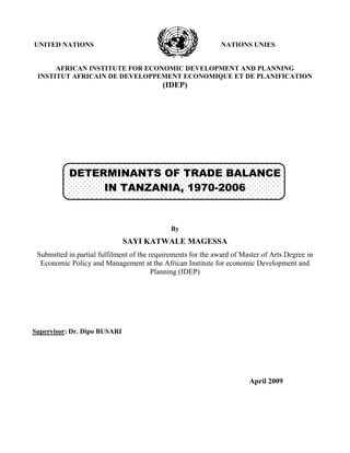
The reforms made
in the early 2000s contributed to the increase in exports, but unfortunately imports were
increasing as well and made the trade balance generally unfavorable 8
(see Figure 2.1).
Figure 2.1: Tanzania merchandise trade balance, 1970-2006 (Tshs millions)
-3500000
-3000000
-2500000
-2000000
-1500000
-1000000
-500000
0
Tshs. (m illions)
1970 1974 1978 1982 1986 1990 1994 1998 2002 2006
Years
TANZANIA MERCHANDISE TRADE BALANCE, 1970-2006
TB
Source: International Financial Statistics of IMF (CD-ROM) and Author’s calculations.
Currently, Tanzania is a member of 2 separate regional trading arrangements (RTAs): the East
African Community (EAC) and the Southern African Development Community (SADC).
Tanzania, however, has not benefited much from these regional and international cooperations as
far as exports are concerned. In general, the major problems that cut across African integration
schemes are more or less the same. These include lack of grassroots support, excessive external
dependency, and institutional weakness, multiplicity of organizations, politics, underdeveloped
economies, the international economic structure and distribution of the benefits of integration.
Paradoxically, these are the same problems that are the very reasons why regional integration in
Africa is on the agenda and will continue to be in the foreseeable future (Nomvete, 1993).
Paradoxically, these are the same problems that are the very reasons why regional integration in
Africa is on the agenda and will continue to be in the foreseeable future (Nomvete, 1993). These
explanations are true for the case of Tanzania. Generally, Tanzania seems to be a marketplace for
goods from her trading partners since it imports more than exports.
7
http://www.nationsencyclopedia.com/economies/Africa/Tanzania-INTERNATIONAL-TRADE.html)
8
Sources: United Republic of Tanzania Economic Survey, 2007

7
Table 2.1: Tanzania’s Value of Exports, 2000-2006 (USD Million)
2000 2001 2002 2003 2004 2005 2006
Traditional
commodity
Coffee 837 571 362 498 498 743 614
Cotton 380 337 286 412 746 1,115 568
Sisal 56 67 66 73 72 73 61
Tea 327 290 296 248 601 256 310
Tobacco 384 367 565 398 576 808 662
Cashew nuts 844 566 466 418 681 466 394
Cloves 100 123 42 103 103 85 82
Sub -Total 2,928 2,321 2,083 2,150 3,277 3,546 2,691
Non
Traditional
Commodity
Petroleum 00 00 00 00 00 00 00
Minerals 1,782 3,022 3,838 5,522 6,802 7,113 8,368
Manufactured
Goods
434 562 659 838 1,101 1,561 1,958
Other
Exports
1,489 2,619 3,239 3,597 3,851 4,544 4,383
Sub Total 3,705 6,203 7,736 9,957 11,754 13,218 14,709
Grand Total 6,333 8,524 9,819 12,107 15,031 16,764 17,400
Source: United Republic of Tanzania, Economic survey, 2007.
A striking feature of the Tanzania growth experience is that when one juxtaposes the respective
growth trends, investment and growth hardly seen to correlate. This was mirrored by the
significance losses in investment productivity during 1970s and early 1980s.It reduced the
economy wide rate return from nearly 30 percent in the early 1970s to nearly 5 percent in the mid
1980s.the economy only slowly recovering from that loss. Underutilization of capacity and poor
investment choices were the main culprits
(Mutalemwa and Ndulu 2002)
CHAPTER THREE: LITERATURE REVIEW

8
3.1 Introduction
The balance of payments is one of the most heavily studied areas in economics. Attempts to
analyse the balance of payments have focused mainly on the determinants of the current account
components, (Farugee and Isard, 1994). This is largely because it is an important macroeconomic
variable whose movements provide information about the behaviour of all market participants in
an open economy. Current account balance is a key leading indicator of the health of a country’s
economy. Movements in this macroeconomic variable are deeply intertwined and convey
information about actions and expectations of all market participants in an open economy. In
particular, the behaviour of the current account balance provides useful insights about shifts in
the stance of the macroeconomic policy and other autonomous shocks, (Knight and
Scacciavillani, 1998). Understanding the behaviour of these economic agents and therefore
movements in the trade balance of payment is an important step in macroeconomic policy
analysis. The balance of payment in analytical terms perhaps is the single most revealing
reflection of the health status of an open economy. In other words, the balance of payments crisis
facing the economy can be seen as a mirror of its underlying economic problems. Contemporary
creditors, for instance, use the balance of payments crisis as a warning indicator for deep-seated
economic crises before contemplating any intervention in the economy (Helleiner, 1986).
A rich body of the literature argues that trade flows respond to currency changes with some
delay (Magee, 1973). Specifically, the short-run effects of currency depreciation is said to be
different from its long-run effects. In the short-run, since goods in transit have been priced at old
exchange rates, the trade balance could deteriorate even after currency devaluation or
depreciation.9
Once the effects of new exchange rate are realized, we may observe an
improvement on trade balance.10
We study both the short- and the long-run linkages between real
exchange rate movements and trade balance in Tanzania.
The export theory can be classified under the neoclassical growth models. The underlying
argument of the export theory is that countries need to export goods and services in order to
generate revenue to finance imports which cannot be produced. Normally, Gross Domestic
9
For more details see Magee (1973) who observed deterioration in the U.S. trade balance despite devaluation of the
dollar by 15% in 1971
10
Following studies investigate the reasons for such depreciation see Bahmani and Kutan (2007)

9
Product (GDP) is used as a proxy of a country’s economic strength and it provides an estimate of
the value of goods and services produced in a country in a specified period.
(Temple, 1994), indicates that because of the demands of international markets such as
continuous innovation and improved efficiency, there is increased specialisation which
encourages utilisation of economies of scale. The export theory thus predicts that growth in
exports causes economy wide productivity gains which amounts to enhanced gross domestic
product. In addition, exports can also be linked to sustainable economic growth through the
balance of payments. The constraints on the balance of payments arise when a country’s level of
imports exceeds that of exports. In such a situation, the deficit can only be financed either
through government borrowing or use of the country’s reserves.
In literature, there are various complementary approaches that have been developed to analyse
the current account. In this review I shall focus on these approaches that are relevant to the
analysis of the current account of Tanzania, which is the focus of the study. In addition to the
theoretical approaches, there is a wide range of literature comprising empirical analysis of the
various models. In this regards, I review both the theoretical and empirical literature on the
balance of payments. The empirical literature review will focus mainly on those studies relevant
to small open developing economies such as Tanzania.
3.2. Review of Theoretical Literature
The history of balance of payment theory since 1930s has been successive approaches of
increasing degrees of theoretical sophistication. In this study I shall provide a summary of the key
issues relevant to my work.
3.2.1 The Elasticities Approach
The approach is based on the Marshallian partial equilibrium analysis of the markets for exports
and imports. Its main preoccupation is in analyzing the effect of devaluation on the trade balance
and in determining the condition under which devaluation can be successful in improving the
balance of payments.11
.The simplest formulation of the approach is based on a partial equilibrium
11
For a more detailed review of such literature, see Goldstein and Khan (1995)

10
model in which the trade balance is expressed in terms of the different between exports and
imports. Using simple export and import demand functions in which the exchange rate and the
prices of imports and exports are important explanatory variables, the conditions under which
devaluation can influence the trade balance are derived in terms of elasticities of supply and
demand for a country’s exports and imports. These elasticities are formulated in terms of the
Marshall-Lerner condition12
which stated that for devaluation to improve the balance of
payments, m
x e
e  13
should be greater than one. See for example, Bahmani-Oskooee (1986)
.Some other studies, such as Shirvani and Wilbratte (1997), Bahmani-Oskooee (1985) Rose
(1991) and Himarios (1989) have constructed a direct link between the exchange rate and the
trade balance. This is based on the assumption of a stable foreign exchange market. If the sum is
equal to unity, a change in the exchange rate will leave the balance of trade unchanged. If the
sum is smaller than unity, depreciation will make the balance of trade unfavorable and an
appreciation will make it more favorable.
The elasticity approach has been criticized on a number of grounds. Firstly, it is based on a partial
equilibrium framework that assumes full employment, price flexibility, and initial equilibrium.
The approach assumes that the economy is initially in equilibrium and thus ignores the fact that
devaluation is mainly undertaken when there are imbalances in the current account. Whether
devaluation leads to an improvement in balance of payment or not depends on the sum of the
foreign elasticity of demand for export and home elasticity of demand for exports x
e and m
e
imports respectively (Johnson, 1972).
A similar critique has been in relation to lags in response of the current account to relative price
changes because of the inertia of importers switching domestic expenditure away from imports
and existence of contracts. In the short run, therefore, devaluation may not increase domestic
export earnings enough to offset the initial increase in the value of expenditure on imports. This
leads to the ‘J effect’ on the current account, where following devaluation, the balance of trade
worsens before it improves in the long run. (Magee, 1973)
12
The Marshall-Lerner condition is originally due to Bickerdike (1920), but has been named after Marshall, the
father of the elasticity concept, and Lerner (1944) for his later exposition of it. For a simple discussion of this
approach see Alexander (1952).
13
Where x
e and m
e foreign elasticity of demand for export and home elasticity of demand for exports imports
respectively.

11
3.2.2 The Absorption Approach
The absorption approach puts emphasis on the income effects of devaluation. As developed by
Alexander (1952), the country’s foreign surplus depends on extend to which domestic output
supply exceeds absorption14
. From his definition of the current account as the excess of income
over expenditure, it was reasoned that for devaluation to improve the current account it needed to
have an impact on either income or absorption. The main conclusion that can be drawn from the
absorption is that the current account can improve if devaluation can generate expenditure
reducing and expenditure switching effects. Expenditure switching can occur only if elasticities
are sufficiently high. On the other hand, expenditure reduction occurs through changes in real
income. Expenditure switching occurs through the effect of devaluation on the relative prices of
foreign and domestic goods, a devaluation increases the demand of domestic goods by foreigners
and at the same time this reduce the demand for imports. This improves the balance of payment.
The main difference between the elasticities approach and absorption approach is that the latter
incorporates the general equilibrium, while the former does not. Though the two approaches are
different, they have the same weakness of not taking consideration of the inflationary effects of
devaluation. Also they do not take into account of the role of money determination of the balance
of payment (Johnson, 1972).
3.2.3 The Monetary Approach
The main idea behind the monetary approach is that balance of payments determination is purely
a monetary phenomenon. A balance of payment deficit or surplus would occur if there were
disequilibrium in the demand and supply of money. These imbalances would be reflected in the
international reserves.15
Under a system of a fixed exchange rate, excess money supply induces
increased expenditure, which shows itself in increased purchases of foreign goods and services
by domestic residents. The purchases have to be financed by running down foreign exchange
reserves thereby worsening the balance of payments. The outflow of foreign exchange reserves
14
For more detailed literature review on Elasticity and Absorption see Johnson (1972)
15
For more detailed literature review on Monetary Approach see Johnson (1972)

12
reduces money supply until it is equal to the money demand thereby restoring monetary
equilibrium and halting an outflow of foreign exchange reserves (Johnson, 1972).
The monetary approach has not gone without criticisms like the other theoretical approaches. Its
applicability to developing countries has been questioned based on the assumptions implicit in
the approach. Long run situation with fully flexible prices, and ignoring of short run adjustment
while taking consideration of only equilibrium points. It is also assumed the demand for money is
stable and that the money market clears automatically which is not realistic especially in less
developed countries. Also, the monetary approach has been criticized on the grounds that, it does
not distinguish between traded and non-traded goods because of assumption of the ‘law of one
price’ that domestic prices of all goods are in line with the international prices (Johnson, 1972).
3.2.4 Structuralist Approach
The core of the structuralist approach is the attempt made in explaining why orthodox
stabilization policies may not achieve their goals as predicted. The initial set of structural
hypothesis was formulated in 1950’s by writers such as Paul Rosenstein-Rodan, W.Arthur Lewis,
Paul Prebisch, Hans Singer and Paul Gunnar Myrdal (Chenery, 1975). One key element of the
formal structuralist models is that devaluation might not induce the expenditure reducing and
switching effects predicted by orthodox models of balance of payments. The explanation is that
due to low elasticities of demand and supply and structural rigidities, appropriate adjustment may
not occur in most development countries. Consequent upon this, devaluation may lead to a
worsening of the current account. However, some empirical studies such as Khan and Knight
(1983) have shown that there are cases where supply and demand responses are adequate for
devaluation to work.
Another explanation from the strucuralist perspective is that devaluation has contractionary
effects, which operate on output through the demand side. Through this channel devaluation
reduces real wages, and thus redistributes income from low savers to higher savers particularly
from workers to capitalists, and consequently reducing domestic absorption. For economies

13
dependent on foreign investment, part of the income redistributed to capitalists is repatriated.16
.Also, the effect on supply may be due to high interest rates as a result of restrictive monetary
policy. When interest rates increase at the same time devaluation takes place, the cost of working
capital increases and since the cost of imported inputs increase as a result of devaluation, then
devaluation and stringent monetary policy will combine leading to a contractionary effect
(Chenery, 1975).
One key weakness of structuralist approach is their behavioural equations are not based on an
optimization framework by economic agents, but on ad hoc assumptions concerning economic
behaviour. The parameters used in empirical research are therefore chosen arbitrarily with little
recourse to the postulates of optimizing behaviour.
3.2.5 Computable General Equilibrium Models
Computable General Equilibrium Models (CGE) is based on the Walrasian general equilibrium
analysis and the neo classical principles of optimization. They model economic behaviour as an
outcome of decentralised decision making by consumers and producers. They assume a perfectly
flexible price mechanism through which adjustment takes place to equate supply and demand in
all markets. The salient feature of CGE models is the derivation of the demand and supply
functions from optimizing behaviour. They also take into consideration the interdependence of
markets and their implications with respect to policy interdependency. Depending on the need
and the extent of data availability, the CGE models can be disaggregated to as many sectors as
possible. (Chumacero and Hebbel, 2005)
Modifications have been made to include market imperfections in the goods, labour, money and
exchange markets. Also, assumptions in respect of substitution mechanisms between exports and
domestic sales have been made. These are introduced in the model by exogenously imposing
structural rigidities like fixed exchange rates, fixed wages and zero elasticities of substitution.
Despite the salient features mentioned above, they have some limitations as regards applicability
to developing countries. In the derivation of the demand and supply functions from an optimizing
procedure, market imperfections should be treated as extra constraints. But, the market
16
For a more detailed treatment of Structual approach see Chenery (1975)

14
imperfections are treated in a simplistic manner. This may result into increased problems of
computation17
. One other limitation is that they do not take account of inter-temporal nature of
many economic decisions. (Chumacero and Hebbel, 2005)
3.2.6 The Mundell-Fleming Model
The Mundell-Fleming (M-F) model is an economic model first set forth by Robert Mundell and
Marcus Fleming. The model is an extension of the IS-LM model. Whereas IS-LM deals with
economy under autarky, the Mundell-Fleming model tries to describe a small open
economy18
.The Mundell- Fleming (M-F) model is a tool that has been used over the years to
analyse how various policy options can be used to attain internal and external macroeconomic
equilibrium. The analytical foundations of the model are founded on a framework that shows the
conditions under which equilibrium can be attained in the markets for goods, money and foreign
exchange. External and internal equilibrium is attained where the IS and LM and BOP lines
intersect.Mundell (1963) and Fleming (1962)
Typically, the Mundell-Fleming model portrays the relationship between the nominal exchange
rate and the economy output (unlike the relationship between interest rate and the output in the
IS-LM model) in the short run. The Mundell-Fleming model has been used to argue that an
economy cannot simultaneously maintain a fixed exchange rate, free capital movement, and an
independent monetary policy Obstfeld (2001). In terms of current account determination, the
Mundell- Fleming model can be used to show how various policy options or changes in other
exogenous factors are transmitted to current account. For example, the model shows that starting
from a current account balance; an expansionary fiscal policy would lead to a current account
deficit. Such a deficit is measured by capital inflows that result from the impact of fiscal
expansion on income and money demand. If the exchange rate is fixed, changes in domestic
credit will have little impact on current account balance (Obstfeld, 2001).
The Mundellian idea of the policy mix was a major conceptual advance and seemingly offered an
elegant way to avoid unpleasant tradeoffs. But the approach had at least two theoretical
17
For more detailed General Equilibrium Models see Chumacero and Hebbel (2005).
18
See Mundell (1963) and Fleming (1962)

15
drawbacks. First, Mundell’s theoretical specification of the capital account as a flow function of
interest-rate levels (a formulation used by Fleming 1962 as well) was theoretically ad hoc. It
implied, implausibly, that capital would flow at a uniform speed forever even in the face of a
constant domestic-foreign interest differential. The second problem, already mentioned, was the
definition of external balance in terms of official reserve flows, rather than in terms of attaining
some satisfactory sustainable paths for domestic consumption and investment. As a medium-term
proposition, it would be unattractive, perhaps even infeasible, to maintain balance-of-payments
equilibrium through a permanently higher interest rate. The results of such a policy–crowding out
of domestic investment and an ongoing buildup of external debt–would eventually call for a
sharp drop in consumption.19
While Mundell’s framework was perhaps useful for thinking about
very short-run issues (such as the need to maintain adequate national liquidity), it failed
completely to bridge the gap from the short run to the longer term. Indeed, the theory of the
policy mix had little practical significance under the Bretton Woods. In his detailed study of nine
industrial countries’ policies during the postwar period to the mid-1960s Michaely (1971) found
only two episodes in which the prescription of the Mundellian policy mix was consistent with the
official measures authorities actually took. Most of the time, Michaely concluded, fiscal policy
simply was excluded from the list of available instruments.20
3.2.7 Macroeconomic-Balance Approach
The analytical foundations had been established in the 1950s by Metzler (1950) and Mundell
(1963) but the application of the model gained importance in the mid 1980s when shifts in fiscal
19
Meade (1951) recognized clearly that in choosing between monetary and fiscal policy, “the
question of the optimum rate of saving is involved.” Mundell briefly discusses problems of the
composition of the balance of payments in chapter 10 of his 1968 book, likening them to
problems of the proper division of national product between consumption and saving. Purvis
(1985) includes a nice discussion of fiscal deficits and the external debt burden from the
perspectives of the Mundell-Fleming and subsequent models.
20
For a more detailed discussion of practical problems in deploying fiscal policy, see Obstfeld
(1993).

16
policy in many industrialized countries became associated with medium term pattern in the
current account balances and exchange rate movements (Knight and Scaccievillani, 1998).
A final important branch in these dynamic developments was the application of optimal growth
theory, in the style of Cass, and Koopmans, to open economies. Notable contributions along these
lines were made early on by Bardhan (1967), Hamada (1969), and Bruno (1970). Building on
these approaches in the early 1980s, a number of researchers developed an intertemporal
approach to the current account in which saving and investment levels represent optimal forward-
looking decisions.21
The new approach contrasted with the Keynesian approaches in which net
exports are determined largely by current relative income levels and net foreign interest payments
are, for the most part, ignored. These new models, unlike the earlier open economy growth
models, were applied to throw light on short-run dynamic issues such as the dynamic effects of
temporary and permanent terms-of-trade shocks and not just the transition to a long-run balanced
growth path. They could also be used to think rigorously about the policy implications of national
and government intertemporal budget constraints. The intertemporal approach, unlike the
Keynesian or monetary approaches, provided a conceptual framework appropriate for thinking
about the important and interrelated policy issues of external balance, external sustainability, and
equilibrium real exchange rates (for a recent example, see Motel, 1999). All of these concepts are
intimately connected with the intertemporal tradeoffs that an economy faces. Another major
advantage of the intertemporal approach was its promise of a systematic welfare analysis of
policies in open economies an analysis on a par, in rigor, with those already applied routinely to
intertemporal tax questions. The approach shifts attention from automatic adjustment
mechanisms and dynamic stability considerations to intertemporal budget constraints and
transversality conditions for maximization, although those perspectives may well, of course, be
mutually consistent (Obstfeld, 2001).
As already reviewed, most theoretical approaches mentioned above are partial equilibrium
approaches whose remedy to balance of payments problems is reliance on devaluation as a policy
option. In addition, while some of these theories consider the distinction between tradable and
non-tradable, other does not. As contrasted to the traditional approaches, of recent the
21
For a more extensive survey of the area, see Obstfeld and Rogoff (1995).

17
structuralist approach has been formulated in a manner that considers the structure of the
economy an important factor and also permits to build in the role of imported inputs as well as
traded and non-traded goods. Though the approaches seem each mutually exclusive in its
theoretical framework, it is evident they are considerably complementary. Thus, a balance
assessment of each approach would suggest the approaches are not conflicting. There is growing
consensus that not a single approach can adequately explain the balance of payments and the
mechanism of addressing the imbalances. Therefore, an integrated approach in which the relative
price, absorption, monetary and structural features are examined would be most appropriate.
3.3 Review of Empirical Literature
The literature on empirical determinants of the current account in LDCs is limited. This is
particularly so in the case of Africa, particular in Tanzania. Available studies tend to be partial in
that they choose a particular theoretical approach and test it empirically. In this way, the studies
focus on the theoretical aspect of the particular approach and thus leave out some other
determinants of the current account in other models. One of the key approaches in the empirical
analysis of the determinants of current account has been through the estimation of the import and
export equations. In addition to identifying the empirical determinants of the current account,
such studies attempt to test the validity of the Marshall-Lerner condition. While providing an
important contribution to the literature, these studies suffer from a number of weaknesses. They
are partial in nature because they consider only the independent variables that enter the import
and export equations.22
. A comprehensive survey of this literature is available in Goldstein and
Khan (1985).
According to Goldstein and Khan (1985), the available evidence shows that for most of the
developing countries studies, the Marshall-Lerner condition was largely met. In an attempt to
address the weaknesses in these studies, Khan and Knight (1983) developed a framework to
examine empirically the influences of external and internal factors on the evolution of the current
account of non oil developing countries during the 1970s. They specified a simple model relating
the current account to its main determinants and estimated the relationship for 32 countries
during 1973-80. Using pooled time series data for 32 countries, they estimated model using least
22
A comprehensive survey of this literature is available in Goldstein and Khan (1985).

18
squares dummy variable technique. The independent variables used in the model were terms of
trade, growth of the GNP of industrial countries, real foreign interest rate, real effective exchange
rate, fiscal position, and time trend. The results of the study showed that both internal and
external factors were important in influencing the current account balance of the countries
studied. The coefficients of the explanatory variables had the expected signs and the overall fit of
the model was good.
In a follow-up study, Doroodian (1985) argued that Khan and Knight failed to take into account
the heterogeneity of the countries in terms of their GNP growth rates, stages of economic
development, and the composition of foreign trade. Also, he argued there were important
explanatory variables that had been left out by Khan and Knight. Doroodian therefore developed
an extended model in which he distinguished between net oil exports and oil importers, which he
in turn classified as exporters of manufactures, low-income countries, and net oil importers. He
also added the income growth rate of the home country and foreign reserves scaled by imports as
explanatory variables.
Using a model similar to that of Khan and Knight (1983), Doroodian estimated the determinants
of current account balances for the groups of countries he had identified. However, he allowed
for the possibility of heteroskedasticity. The results showed that all the variables other than
foreign reserves had the expected signs and were statistically significant. Also, he showed that
the ratio of foreign reserves to imports had the same effect on the current account except for other
net oil importers. The analysis also showed that major exporters of manufactures were more
vulnerable to external shocks and that this could explain why such countries experienced large
current account deficits during the period studied.23
In another study similar to that of Khan and Knight (1983), Germann and Mann (1989) undertook
to estimate empirically the determinants of current account in selected Latin American countries
for period 1973-84. Although their focuses were on the determinants of external debt in these
countries, they used the current account balance scaled by exports as the dependent variable
23
The variable for growth rate differential was included on the basis that the volume of trade is affected real income growth in
home country as well as in its major trading partners. It was reasoned that if the income of the home country grew faster than of
its major trading partners, then the home country could have a trade deficit, given that income elasticities are the same in both
countries. (See IMF staff papers, Volume 32, number 1, March 1985 pp. 160-164)

19
arguing that this was a reasonable proxy for debt. As found in other studies, their results showed
that both external and internal factors were statistically significant in explaining the current
account.
Bartoli (1989) undertook to empirically analyse how fiscal policy transmits itself to the current
account balances using a general equilibrium framework, she developed a five equation system
comprising government current expenditure, government current revenue, total investment,
domestic savings and the current account. She estimated the system using panel data for the
period 1973-83. The method of OLS with dummy variables was used in order to take into
account cross-country differences. The key finding in this study was that the financing of the
budget exerted a large negative effect on the current account. The results of current account
equation showed that the short run movements of the current account were determined by
inflation tax and government capital expenditure with the former affecting private savings
negatively while the latter exerted a multiplicative effect on investment. Real domestic and
foreign interest rates were among the financial variables that appeared to worsen the current
account, through their effect on the current government expenditure.
Despite the popular belief that depreciation can improve trade balance, empirical works tend to
suggest mixed results. Amongst 30 countries studied, Rose (1990) finds that the impact of
devaluation on trade balance is insignificant for 28 countries, and one country shows negative
impact. He concludes that devaluation does not necessarily lead to an increase in trade balance.
More recent work by Upadhyaya and Dhakal (1997) also suggests that improvement in trade
balance was only found in one country out of eight countries studied. On the other hand, others
like Bahmani- Oskooee (1991) and Himarios (1989) find trade balance improvement following
currency devaluation.
Elbadawi and Solo (1977) worked on several developing countries (Ghana Kenya, Mali, Cote
d’Ivorie, Chile, India and Mexico). They employed the standard Dickey Fuller Test to test for the
unit roots tests in all variables. With the exception of the short term capital inflows, all
fundamentals present evidence of non stationary. The Granger test shows that, the real exchange
rate (RER) is Granger caused fundaments, except for the public investment. For most countries,
the causation goes from the real exchange rate to public investment. This signals that public

20
investment is not an adequate proxy for the fraction of government expenditure in the non
tradable goods. They used Engle and Granger (1987)’s two steps procedure to estimate the long
run cointegrated equilibrium. The degree of openness of the economy, defined as the sum of
exports and imports as a ratio to the GDP was found to be important. In all countries a negative
coefficient supports the notion that reforms aimed at reducing tariffs and eliminating trade
restrictions are consistent with a more depreciated real exchange rate.
Saruni (2006) worked on determinants of Trade balance in Tanzania for the period from 1970 to
2002. Although he didn’t incorporate short run dynamics and long run steady which can be
incorporated by using error correction mode, he found that FDI has positive relationship on trade
balance. He found that a 10.0-unit increase of FDI will result in a 0.8-unit improvement in the
trade balance in Tanzania. The impact, however, is not very significant because much of the so-
called FDI currently in Tanzania is in the form of imported capital equipment, and not much has
been produced for export so far.
In a separate study, both the relationship between fiscal deficits and macroeconomic
performance of eight developing countries Easterly and Schmidt- Hebbel (1993) found slightly
different results. High government spending was found to result in an appreciation of the real
exchange rate for Argentina, Coted’Ivorie and Morocco. In the case of Chile, Colombia and
Mexico it resulted in depreciation. Elbadawi (1992) developed a real exchange rate determination
model to account for the traditional long run real determinants such as terms of trade and
commercial policy on the Sudanese economy. The model incorporates the effect of domestic
absorption, which reflects the impact of excess aggregate demand in the economy. The results
provide strong support to the prediction of the cointegration technique. Foreign prices are shown
to have significant influences on the equilibrium level of real exchange rate. The long run effect
of domestic absorption (proxied by the log of total domestic credit) is also quite significant with
an elasticity of o.57. Nominal devaluation was found to have no effect on the process of real
depreciation if implemented from a position of overvaluation.
From the review of empirical studies undertaken by various scholars, one can arrive at a number
of conclusions. Most of the studies have either attempted to test a particular theory empirically on
an individual country or a cross-section. But others have adopted a strategy where they combine

21
various elements of different theories to suit characteristics of a given economies. Most of the
studies reviewed employed econometric techniques to analyse the data of countries concerned.
However, some have employed statistical methods and trend analysis. In view of the different
studies reviewed, there is need to adopt an integrated approach to the analysis of the current
account of the balance of payments.
Based on the above consideration, it can be argued that there is no single unifying framework for
the analysis of the current account of the balance of payments. As noted by Karunartne (1988),
the lack of theoretical guidelines has led to an amalgam of historical and eclectic approaches to
identify and estimate the key determinants of current account balances in developing countries.
This is an important issue particularly when it comes to prescribing appropriate policy
prescriptions. Note that while some studies have used aggregate trade data, some have employed
bilateral trade data. Again, the findings are mixed (Bahmani and Kutan, 2007)
Frankly speaking, the factors influencing current account of balance of payments have been
viewed in terms of external and internal shocks and how to deal with them by creating a
mechanism to minimize or avoid these shocks.

22
CHAPTER FOUR: METHODOLOGY, RESULTS AND
INTERPRETATION
4.1 Introduction
The research methodology employed in this study is based on literature reviewed above and a
model was selected that best represents the circumstances of African countries and, in particular
Tanzania. Moreover, the model is selected to take into account the specific features of Tanzania.
The modification made was in terms of explanatory variables. This modification will be
discussed in the sections that follow.
4.2 Model Specification
Due to the fact that there is no single unifying framework for the analysis of the current account
of the balance of payments, the literature suggests that the internal and external factors that
influence an economy’s trade balance vary from country to country and from time to time. As a
result, their influences on the trade balance also vary significantly. A full account of such factors
requires a detailed country analysis. It is therefore important to establish an empirical relationship
between Tanzania’s trade balance and its determinants. In this study, the approach chosen for my
work is based on the work by Bahmani-Oskooee (1985), who introduced a simple reduced form
model of the trade balance in which the trade balance was related to the real exchange rate,
foreign income and domestic income.
A country’s trade balance equation can be expressed in a reduced form as follows:
TB = f (RER, YW, FDI, G, OPEN, HC) Brada et al. (1997) model............................. (4.1)
On equation 4.1 above, Trade Balance was expressed as a function of all the key determinants
and taking into account both internal and external factors. The consensus among all recent studies
is that the trade balance should depend on a measure of domestic income, a measure of foreign
income and the real exchange rate. Thus, following Rose and Yellen (1989) and many other
studies, in order to run the regression analysis from the above function; I model Tanzania’s trade
balance as follow:
t
t
t
t
t
wt
t
t LogHC
a
OPEN
a
LogG
a
LogFDI
a
LogY
a
LogRER
a
a
LogTB 








 6
5
4
3
2
1
0 ….…
……………………………………………………………………………………..4.2

23
Where
TB is a measure of the trade balance. Following Bahmani-Oskooee (1991) and others we define it
as the ratio of imports over exports so that the model could be expressed in log-linear form at
time t,24
RER is the measure of real effective exchange rate at time t,25
( wt
Y ) is a measure of foreign income,26
FDI is foreign direct investment at time t in U.S
dollars, t
G is Government expenditure at time t, OPEN (commercial policy) is the sum of exports
and imports as a ratio of gross domestic products, t
HC is household expenditure at time t
(including net private investment and t
 -is the error term, included in the model to capture
unexplained factors in the trade balance.
Although the analytical structure remains the same as the one in Bahmani-Oskooee and Brada et
al, my model has been modified by including in the model foreign direct income, Government
expenditure, Openness and Household expenditure. Introduction of new variables in the model is
based on the three assumptions suggested by Branson (1983).First the neoclassical assumption of
price and wage flexibility guarantees full employment. Next in the global market, "the law of one
price" would lead to an equalization of the domestic and foreign currency price of each good.
Finally on the assumption that domestic and foreign financial assets are perfect substitutes,
foreign and domestic interest rates would be equal except for anticipated exchange rate changes.
Therefore, these variables are significant and necessary to include into the model to be
estimated.27
24
The ratio is used to make the measure of trade balance unit free (Bahmani-Oskooee, 1991). For theoretical
derivation of the reduced form see Rose and Yellen (1989, pp. 54-55).
25
I note that data on real effective exchange rates in LDC’s is hard to obtain. In this study, I used NER=Nominal
Exchange Rate to compute Real Growth Exchange Rate as RER= (NER*CPI Domestic/ ICPI Foreign CPI). Where CPI=
Consumer price Index and ICPI= Indian Consumer Price Index, (Tanzania major trading partner).
26
Foreign income, calculated on the basis of Tanzania’s five major trading partners that account for the largest
shares of its trade namely; India Japan, China, South Africa and Kenya.
27
A comprehensive survey of this literature is available in Branson (1983).

24
4.3 Justification of Variables
TB is a measure of the trade balance. Following Bahmani-Oskooee (1991) and others defined it
as the ratio of imports over exports so that the model could be expressed in log-linear form at
time. If a decrease in REX or depreciation is to lower imports and stimulate exports, therefore
RER have positive impact on the trade balance28
.
Household expenditure depending on the scene of economic growth plays a critical role. If the
level of an economy’s output is expected to rise permanently in the future, households in the
economy may smooth out consumption by borrowing more and thus lead to an increase in current
account deficit or reduction of surplus29
. Thus household expenditure will be a negative function
of the trade balance.30
The expansion in the final goods component of government expenditure produces a sizeable
worsening in the current account balance of the home country and corresponding increases in net
foreign indebtedness. Therefore, conditional on a positive shock to domestic government
expenditure on final goods, the current account deterioration in the home country appears
noticeably linked to the increase in government expenditure.31
Thus, Government expenditures
therefore have a negative impact on the trade balance
The economic impact of FDI on the level of economic activity has been widely investigated in
recent years across different countries. Some results suggest that the inflow of FDI can ‘crowd in’
or ‘crowd out’ domestic investment depending on specific circumstances. Overall, FDI has a
positive impact on economic growth but the magnitude of the effect depends on the availability
of complementary resources, especially on the domestic stock of human capital (Vaidya, 2006).
Empirical research in several countries suggests that the initial inflow of FDI tends to increase the
host country's imports. One reason for this is that primarily FDI companies have high
propensities to import capital and intermediate goods and services that are not readily available in
28
See Bahmani and Kutan(2007)
29
Paper presented at CES/AEA session at ASSA 2003, Washington DC by Lu and Ding*
30
For more detailed discussion see Bahmani (1991)
31
For a more extensive survey of the area, see Cavallo (2005)

25
the host country. However, if FDI is concentrated in import substituting industries, then it is
expected to affect imports negatively because the goods that were imported earlier would now be
produced in the host country by foreign investors Vaidya (2006). The impact of FDI on the trade
balance may be positive or negative.
Income from the rest of the world it has a positive impact on the trade balance. The fundamental
assumption is that when the income of Tanzania trading partner’s increases, they would import
more from Tanzania (Rawlins and Praveen, 1993)
Openness variable (Commercial policy) affects trade balance depending on the brutality of trade
restriction and exchange controls. Trade restrictions and exchange controls reduce the degree of
openness of domestic economy, thereby reducing the relative prices of importable goods to non
tradable goods, thus causing the exchange rate to appreciate. Given the difficulties of obtaining a
well defined measure of trade restrictions and exchange control most empirical studies use the
ratio of the sum of exports and imports to gross domestic product (open) as a proxy. The variable
is expected to carry a positive sign (Bhorat, 2000).
4.4 Empirical Analysis
Economic theory requires variables in regression analysis to be stationary. Engle and Granger
(1987) have shown that ordinary least squares (OLS) estimators can be inconsistent when
economic time-series are not stationary and consistent with the assumptions of the linear
regression model (LRM). Although OLS estimation can give results with high 2
R and significant
t-statistics, inferences based on traditional statistical tests could be misleading. For modeling
purposes, I tested the stationarity of the time-series before conducting regression analysis. I also
tested whether the assumptions of the LRM are violated and correct them accordingly.
The trade balance model expressed by equation (4.2) above represents the long-run relationships
between the trade balance and its determinants. In an effort to test the trade balance deficit I
incorporated the short-run dynamics into the long-run model outlined by equation (4.2). The
easiest way to do this is to express equation (4.2) in an error-correction modeling format. I do this
following testing approach of the general mathematical formulation of the Hendry ECM model.
The general mathematical formulation of the Hendry ECM model is as shown below:

26
t
k
t
k
t
t
t
kt
k
t
t
t X
X
X
Y
X
X
X
Y 







 













 


 ....
.... 2
2
1
1
1
0
2
2
1
1
0 ..... (4.3)
 
 

 






k
i
k
j
t
jt
j
t
it
t X
Y
X
Y
1 1
1
1
0
1
0 



 ……………………………………. (4.4)
Where:
0
 = constant
0
 = error correction coefficient
k


 ,...
, 2
1 = short-term dynamics
k


 ,...
, 2
1 = long-term dynamics
Hence the linear specification of our error correction model is as below:
            OPEN
D
a
LFDI
D
LYw
D
LG
D
LHC
D
LRER
D
LTB
D (
6
5
4
3
2
1
0 





 





     
)
5
.
4
(
..
)
1
(
)
1
(
)
1
(
1
1
1
13
12
11
10
9
8
7
t
OPEN
a
LFDI
a
LYw
a
LG
LHC
LRER
LTB



















Wher
e; D= Difference operator, defined as D(X) t = Xt – Xt-1,, 0
 = Constant
t
 = the error term, 6
5
4
3
2
1 ,
,
,
,
, 




 = Coefficients of the short-run model and
13
12
11
10
9
8
7 ,
,
,
,
,
, 





 = Coefficients of the long-run model
As indicated in the previous section, the first task in estimating equation (4.3) is to justify the
inclusion of the lagged level variables by carrying out the F test. It has been demonstrated that the
results could be sensitive to the lag order imposed on each first differenced variable. Thus, as a
fixed rule, following Bahmani-Oskooee and Ratha (2004b), I impose lags on each first
differenced variable and employ Akaike’s Information Criterion (AIC) to select the optimum
lags. I then carry out the F test at optimum
4.5 Scope and Data Sources
The study period covers 1970-2006 which comprises 37 observations for each variable. This
study has relied on secondary time-series data concerning the trade balance (defined as the ratio
of imports to exports).Variables which were investigated involved; household consumption
expenditure, government expenditure, FDI, the real exchange rate, openness (sum of exports and
imports as ratio to gross domestic products) and income from the rest of the world (calculated
using five major Tanzania’s trading partners, namely; India, China, South Africa, Japan and
Kenya).All variables are transformed in to log form except openness. Furthermore, many studies

27
have defined international trade as involving cross-border movement of goods, services, and
factors of production such as capital and labor. This study covers only merchandise trade because
it was difficult to get relevant information on trade in services.
4.6 Limitation of Data
It was not possible to obtain all the data from the one source. The data reported in these sources
are in some cases inconsistent because each source has inherent problems in the data generation
process. However, in order to minimize this problem, where data on a given variable could be
obtained from the same source, I tried to stick to one such source.
4.7 Estimation Procedures
A number of diagnostic tests were carried out to clarify and determine the characteristics of the
data used. The analysis begins with examination of data generating process of each variable. For
this purpose, two unit root tests are used: Phillips-Perron (PP) (1988) and Augmented Dickey-
Fuller (ADF) (1979) tests. The tests are done both in the level, first difference and second
difference of the data and the results are presented in Table 4.2. In all cases, the results provided
by ADF test are consistent to that of PP test. The tests suggest that all variables are non-stationary
in the level and all stationary in the first difference, except income from the rest of the world was
stationarly in the second difference.
Table 4.1: Unit Root Test Results
At level At 1st
Difference At 2nd
Difference Deci
sion
Intercept Trend &
Intercept
Intercept Trend &
Intercept
Intercept Trend &
Intercept
ADF PP ADF PP ADF PP ADF PP ADF PP ADF PP
LTB -2.51 -2.40 -2.40 -2.31 -6.32** -6.68** I(1)
LHC -2.01 -1.75 -2.86 -2.86 -6.04** -9.37** I(1)
LG -0.83 -0.82 -1.79 -1.77 -4.21** -4.27** I(1)
LYW 0.08 0.14 -2.36 -1.90 -2.76 -2.72 -2.78 -2.76 -6.42** -6.55** I(2)
LRER -0.65 -0.42 -1.58 -1.61 -3.12** -3.11** I(1)
LFDI -0.94 -0.56 -2.64 -2.52 -6.82** -7.79** I(1)
OPEN -1.63 -1.92 -2.37 -1.61 -4.25** -4.17**
I(1)
Source: Eviews 6. Note: (**) and (*) denotes stationary at 1% and 5% Level respectively.
ADF is Augmented Dickey-Fuller test and PP is Phillips-Perron test.
Investigation of the long run relationship using Johansen cointegration test, the results were
found to be satisfactory. (See table 4.3)

28
Table 4.2: Johansen Cointergration Test Results
Lags interval (in first differences): 1 to 1
Unrestricted Cointegration Rank Test (Trace)
Hypothesized Eigenvalue Trace Statistic 0.05 Prob.**
No. of CE(s) Critical Value
None * 0.825479 188.9898 125.6154 0.0000
At most 1 * 0.733790 127.8899 95.75366 0.0001
At most 2 * 0.601674 81.56849 69.81889 0.0043
At most 3 * 0.441497 49.35148 47.85613 0.0359
At most 4 0.404650 28.96415 29.79707 0.0621
At most 5 0.199786 10.81292 15.49471 0.2233
At most 6 0.082465 3.012254 3.841466 0.0826
Trace test indicates 4 cointegrating eqn(s) at the 0.05 level
* denotes rejection of the hypothesis at the 0.05 level
Source: Eviews 6
From Table 4.3 above, the Johansen Test indicates 4 cointegrating equation(s) at 5 percent level,
which this implies that I can use the error correction model (ECM) Because of that, I employed a
“two-step” ECM procedure, which permits separate estimation of long-run (steady state)
relationships and short-run dynamics. A keen element in a long run dynamic model of this type is
the coefficient of the error correction model.. The coefficient of the error collection term shows
the expected sign and is significant at 1 percent level of significance. A negative and significant
coefficient obtained for ECM is an alternative way of supporting cointegration. By this criterion,
cointegration is supported in my case, this provides more powerful support for cointegration
among the variable. (See Table 4.4)
Finally, I concluded empirically that errors are homosdakecity, errors are not correlated, the
variables are cointegrated, and the model was well specified, good, and structurally stable and the
overall fit of the model was good. In addition I accepted the results that the trade balance (TB)
and its explanatory variables (HC, G, FDI, OPEN, RER and YW) Series of Tanzania follow
normal law and are lognormal over the period from 1970 to 2006 (see Annex 2-7). Having
completed all the requisite tests I applied OLS to the model to estimate the parameters.

29
Table 4.3: Regression Results
Coefficient Std. Error t-Statistic Prob.
C -12.4338 4.5462 -2.7350 0.0121
D(LFDI) 0.0375 0.0441 0.8516 0.4036
D(LG) 0.9176 0.2947 3.1134 0.0051**
D(OPEN) -0.2480 0.2624 -0.9453 0.3548
D(LYW) 0.7136 0.3095 2.3057 0.0309**
D(LRER) -0.5894 0.1596 -3.6934 0.0013**
D(LHC) 2.2845 0.5555 4.1125 0.0005**
LTB(-1) -0.5099 0.1709 -2.9830 0.0069**
LFDI(-1) 0.0425 0.0544 0.7799 0.4438
LG(-1) 0.5784 0.2192 2.6383 0.0150**
OPEN(-1) -0.4622 0.1283 -3.6030 0.0016**
LYW(-1) 0.2401 0.1264 1.9001 0.0706*
LRER(-1) -0.1878 0.0903 -2.0802 0.0494**
LHC(-1) 1.9557 0.8588 2.2773 0.0328**
R-squared 0.7696 Mean dependent var 0.0197
Adjusted R-squared 0.6335 S.D. dependent var 0.2165
S.E. of regression 0.1311 Akaike info criterion -0.9412
Sum squared residue 0.3778 Schwarz criterion -0.3254
Log likelihood 30.9412 Hannan-Quinn criteria. -0.7262
F-statistic 5.6530 Durbin-Watson stat 1.7803
Probability(F-statistic) 0.0002
Source: Eviews 6. Note: (**) and (*) denotes at 1% and 10% significant Level respectively. L is
the Neperian logarithm: D is the first difference operator defined by D(Xt) = Xt-Xt-1, which
indicates short run effect for specific coefficient of a variable, while (-1) it indicates Long run
effect. G is Government Expenditure; HC is Household expenditure (including net private
investment; OPEN is Openness (commercial policy) is the sum of exports and imports as a ratio
of gross domestic products; RER is Real exchange rate; FDI is Foreign Direct Investment and
YW is Income from the rest of the world
4.8 Interpretation of Results
The general fit of the model was found to be satisfactory with adjusted 2
R of 63 percent. This
implies that up to 63 percent of the variation in the trade balance in Tanzania is explained by
changes in the factors included by the model. The coefficient of the error correction shows a
negative sign as expected, (-0.51) at the 1 percent significant level in a long run. This implies that
51 percent of the effect of the trade balance in Tanzania can be absorbed in the following year.
The probability (F-statistic) is 0.0002 is also small, at 1 percent level which confirms that the
model has significant explanatory power. The constant is significant at the 1 percent level, which
implies that the model had captured many of the factors influencing the trade balance in
Tanzania.

30
From Table 4.4 above; four variables household expenditure, government expenditure, real
exchange rate and income from the rest of the world are statistically significant in explaining the
imbalances of the trade balance in Tanzania. Analyzing the estimated results above, exchange
rate and openness (commercial policy) are the main variables that cause the trade balance deficit
in Tanzania.
RER has negative sign but its effect is significant at 1 percent level both in a short and long run.
A 1 percent increase in real exchange rate results in a 0.6 percent worsening of the trade balance
in a short run. Thus, currency devaluation in a situation of foreign currency scarcity and
substandard export is not a feasible solution for promoting exports. This result is consistent with
study carried by Rose (1990) who concludes that devaluation does not necessarily lead to an
increase in trade balance. Upadhyaya and Dhakal (1997) also suggests that improvement in trade
balance was only found in one country out of eight countries studied. In developing countries like
Tanzania, what is more important is to improve the value of exports such that they will compete
in the world market not only in terms of price, but also in terms of superiority. There is a need
also to improve infrastructure. Although the result was unexpected, this reflects the realism about
the nature of the export product agricultural crops which face deteriorating terms of trade in
Tanzania.
Income to the rest of the world shows a positive sign, as expected, at the 1 percent and 10 percent
level of significance in a short and long run respectively. A1 percent increase in the income of the
rest of the world in a short run will result in a 0.7 percent improvement in Tanzania’s trade
balance. This finding suggests that Tanzania needs to improve productivity and efficiency so as
to meet the standards of foreign demand.
Government expenditure, on the other hand, is not having the expected sign and its effect is
significant at the 1 percent level both in a short and long run. A 1 percent increase in government
expenditure would lead to an improvement of the trade balance by 0.9 percent. According to the
theoretical literature of Taylor (1993), this result simply means that there have been reasonable
government interventions, such as investment in productive sectors, undertaken to encourage
exports. Elbadawi and Soto (1977), in most countries they obtained the positive elasticity of

31
government expenditure implying that fiscal spending tends to appreciate the real exchange rate.
(Ghana Kenya, Mali, Cote d’Ivorie and Chile).
Household expenditure has also indicated a positive sign and is statistically significant at 1
percent level both in a short and long run. This result shows that a 1 percent increase in
household expenditure will result in a 2.3 percent improvement of the trade balance in a short
run. Such a result for Tanzania is not correct and is strongly supported by the high import content
of commodities found on the consumer bookshelf in Tanzania .This is true because there are very
few goods produced locally, compared with local demand. Total demand is fulfilled largely by
imported consumer goods. Even the few locally produced goods that are existing don’t meet the
qualities preferred by local consumers, so there is a lot of substitution of imported goods for
locally produced ones. That substitution continues to worsen the trade balance rather to recover
trade balance.
FDI shows a positive relationship however; its effect is insignificant both in a short and long run
as shown by probabilities. A 10 percent increase of FDI will result in a 0.4-unit improvement in
the trade balance in a short run. This result is consistent with Saruni (2006), who found that a
10.0-unit increase of FDI will result in a 0.8-unit improvement in the trade balance in Tanzania.
The impact, however, is not very significant because much of the so-called FDI currently in
Tanzania is in the form of imported capital equipment, and not much has been produced for
export so far. According to the theoretical literature of Vaidya (2006), this result simply means
FDI has a positive impact on economic growth but the magnitude of the effect depends on the
availability of complementary resources, especially on the domestic stock of human capital.
Empirical research in several countries suggests that the initial inflow of FDI tends to increase the
host country's imports. One reason for this is that primarily FDI companies have high
propensities to import capital and intermediate goods and services that are not readily available in
the host country. These explanations are true for the case of Tanzania.
Openness (Commercial Policy) has indicated negative sign but it is insignificant in a short run
however, it is statistically significant in a long run at the 1 percent level. This means that trade
liberalization had played an important role in influencing the trade balance in Tanzania. The
result shows that the deficit is worsened by 0.3 percent when the country introduces trade

32
liberalization. This result is consistent with the Elbadawi and Soto (1977) they found negative
coefficient of openness which supports the notion that reforms aimed at reducing tariffs and
eliminating trade restrictions are consistent with a more depreciated real exchange rate. By
looking at the real situation in Tanzania, I see that this statement is true since there was a
physically powerful flood of consumer goods after trade liberalization in the early 1990s. There is
evidence to suggest that policy reforms during the 1990s may have attracted the additional
overflow of private capital. Additionally, the increase in FDI from US$11 million in 1998 to
US$474 million in 2006 reinforces the belief that investors responded favorably to policy
changes that took place during the 1990s, this also is consistent with the World Bank (2008).

33
CHAPTER FIVE: POLICY RECOMMENDATIONS AND CONCLUSION
5.1 Summary of Findings
The purpose of this study has been to present the Tanzanian experience with trade deficits and to
identify the main contributions of the policy instruments that were used to confront the problem.
In terms of policy instruments used, it should be noted that the instruments have attracted more
imports (capital outflows), but that domestic capacity to produce for export is inadequate. The
study also has aimed at determining the origin cause of trade deficits that have carry on in
Tanzania since the 1970s. In the case of Tanzania, I have found that the main contributing factors
for trade deficit balance are real exchange rate and openness (commercial policy).
5.2 Policy implications
The key policy implication from this study is derived from the findings that both internal and
external factors were important in determining the Trade balance behaviour in Tanzania. These
results indicate that policymakers in Tanzania may not use exchange rate policy to promote large
balance of trade surpluses and hence economic growth, especially in the long run. This finding
suggests that other policy channels, such as monetary and fiscal policy, become more important
than ever to establish effective means of real convergence towards the world standards.
Therefore, policymakers may need to pay closer attention to the importance of fiscal discipline
and the close coordination of monetary and fiscal policy in Tanzania to achieve economic
growth. Maintaining a depreciated exchange rate not only has implied positive consequences on
the balance of payments through the foreign elasticity of demand and domestic elasticity of
supply of exports, but also through its effects on absorption and monetary aspects. While
elasticities focus attention on the structural or expenditure and resource switching aspects of
depreciation, it effects on the level of real expenditure is also important.

34
5.3 Policy Recommendations
As noted earlier, among of the key variables that were significant in influencing the Trade
balance was Government Expenditure. The policy recommendation here is that in order to
improve on trade balance Tanzania should exercise fiscal discipline. In terms of fiscal discipline,
the key would be to ensure efficient collection of revenue accompanied with strict expenditure
management and controls. Also, expenditures should be geared towards, productive activities that
contribute to growth.
The results show that commercial policy (openness) played a significant role in influencing the
trade deficit balance in Tanzania. To address the problem constraining trade expansion and
growth in Tanzania, it is necessary that the choice of suitable policy instruments reflects the most
direct relationship between issues involved in the identified constraint and the instruments
available. Trade policy implementation has to prioritize the application of instruments to address
specific problems on the basis of anticipated direct impact
Since real depreciation is not effective for Tanzania to achieve economic growth in the long-run,
reducing exchange rate fluctuations, to prevent the real exchange rate from depreciating, it would
be important for Tanzania to maintain a flexible exchange rate system while ensuring that
inflation is kept at a low-single digit level.
As pointed above, both internal and external factors were important in determining the Trade
balance behaviour in Tanzania. As I have noted in the literature, dependence on primary goods
for export has been one of the key reasons why terms of trade have adverse effects in African
countries particularly in Tanzania. In order to minimize this, it will be important for Tanzania to
diversify its exports by increasing her share of manufactured exports in the world trade.
Enhance policies to increase trade with African countries would be useful in diversifying
Tanzania trading partners. While these measures are useful, they need to be implemented in a
comprehensive macroeconomic framework that promotes economic stability and growth. In this
connection, it is important for Tanzania to continue deepening the structural and economic
reforms

35
5.3 Conclusion and Area for further studies
The purpose of this study was to discover most essential factors that bigoted the trade balance in
Tanzania since 1970s and to identify the main contributions of the policy instruments that were
used to confront the problem. These results indicate that policymakers in Tanzania may not use
exchange rate policy to promote large balance of trade surpluses and hence economic growth,
especially in the long run. This finding suggests that other policy channels, such as monetary and
fiscal policy, become more important than ever to establish effective means of real convergence
towards the world standards. Therefore, policymakers may need to pay closer attention to the
importance of fiscal discipline and the close coordination of monetary and fiscal policy in
Tanzania to achieve economic growth. Managing the current account for Tanzania should be
based on prudent economic policies at home and efforts to diversify the economies as well as
diversifying the structure and direction of trade by increasing her share of non traditional goods
and manufactured exports in the world trade.
While this study has advanced the literature on several fronts there are some shortcomings that
will be addressed in future work. The existing literature has revealed several variables that
influence trade balances. I have been able to capture some of them in the Tanzanian context, but I
could not capture others. Variables like terms of trade and capacity to produce for export are very
important in explaining the variability of the trade balance. But a lack of consistent and reliable
data on terms of trade kept me from not capturing its effect on trade balance. If enough reliable
information can be obtained about these variables, integrating them with the other variables
would be interesting work. Trade in services is another important area that needs further research
because it is now the booming industry in the majority of least developed countries. Such
research can also encompass forecasting in sample in order to substantiate one’s empirical
findings.

MAGESSA_Sayi.pdf

Recommended

Recommended

More Related Content

Similar to MAGESSA_Sayi.pdf

Similar to MAGESSA_Sayi.pdf (20)

Recently uploaded

Recently uploaded (20)

MAGESSA_Sayi.pdf