1. Unstructured Grid Generation and Flow Simulation
S. Fatemeh Razavi, Jeff Boisvert, Juliana Leung
University of Alberta, Edmonton, AB
Grid Shapes: Triangles and Tetrahedrons
Mesh Generation Technique: Delaunay Tessellation
Grid Type: Unstructured Grid
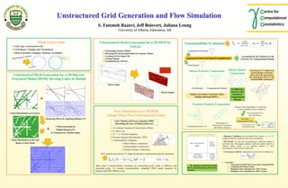
Mesh Generation
Unstructured Mesh Generation for a 2D Discrete
Fractured Model (DFM): Develop Codes in Matlab
0 10 20 30 40 50 60 70 80 90 100
0
10
20
30
40
50
60
70
80
90
100
All Faults
0 10 20 30 40 50 60 70 80 90 100
0
10
20
30
40
50
60
70
80
90
100
G o ts a te e o g C ose o ts
Point Distribution on BG and
Remove Close Points
Point Distribution on Fractures
+
0 10 20 30 40 50 60 70 80 90 100
0
10
20
30
40
50
60
70
80
90
100
Mesh Generated by:
Matlab DelaunayTri
& Visualized by: Matlab triplot
Removing Slivers by Applying Distance CF
+
Unstructured Mesh Generation for a 3D DFM by
TetGen
Generating Fracture Planes
Detecting the Intersections Between Fracture Planes
Creating TetGen Input File
Getting Output
Visualization by TetView
TetGen input
TetGen output
Flow Simulation on a 3D DFM
(Single Phase Flow/Unstructured Grids)
Goal: Solution of Pressure Equation (PDE)
Describing the Flow of Fluid in Reservoir
1) Continuity Equation (Conservation of Mass)
2) Darcy Law
3) 1 + 2 = Pressure Equation
Pressure Equation Discretization: TPFA
Transmissibility Evaluation
Matrix-Matrix Connections
Fracture-Matrix Connections
Fracture-Fracture Connections
TPFA Scheme true for any CV shape (structured or unstructured) and any dimension:
Main point is transmissibility evaluation for unstructured grids which is different with
structured grids. To evaluate transmissibility, simplified DFM model proposed by
Karimi-Fard (SPE 79699) is used.
Transmissibility Evaluation
Accounting for the Thickness of the
Fractures in Computational DomainApplying Karimi-Fard Model for Simplification
Grid Domain
Computational Domain
Matrix-Fracture Connections
Volume correction is necessary when
dealing with large DFM s.
Grid Domain Computational Domain
Matrix-Matrix
Connections
No difference
between Grid
Domain &
Computational
Domain
3 Intersecting Fracture CVs
Intermediate CV:
Intersection of 6 fractures
with different thickness
Fracture-Fracture Connections
Because of the intermediate CV small size,
it causes instability in the calculations
To avoid using CV at
the intersections
Star-Delta
Transformation (SDT)
The equivalent T for n
connecting fractures
Each fracture CV which is not
on the boundary of fracture
plane and in the intersections
has connectivity with 5 CVs for
transmissibility calculations
Matrix - Matrix Assembly
(MMA)
Transient of
Matrix - Fracture
Assembly (MFA)
Matrix –
Fracture
Assembly
Fracture -
Fracture
Assembly
(FFA)
Transmissibility Matrix Structure
Boundary Conditions: For an isolated flow system, “u . n = 0”
condition should be satisfied on the reservoir boundary.
BCGSTAB: To solve the nonsymmetrical coefficient matrix in
each time step, Biconjugate gradients stabilized method could be a
suitable choice which is an iterative method to solve
nonsymmetric linear systems numerically.
Convergence Analysis: mean pressure errors can be computed as:
Extenstion
Unstructured 2D/3D Mesh Generation Using DistMesh,
Completing 3D-1Phase model,
Multiphase Flow Simulation by TPFA scheme,
Multiphase Flow Simulation by MPFA scheme.
By applying Karimi-Fard model
flow is considered along and between
fractures .

2. Effective medium theory
Power law averaging
Arithmetic (horizontal K), Geometric (vertical K), Harmonic mean techniques
Cardwell Parsons
Percolation Model
Hierarchical methods such as renormalization
These techniques are fast but suffering from some limitations
Direct methods also known as pressure solver methods
Histograms
at different
scales
Effective
property vs.
Scale: in x
direction (100
realizations)
Permeability Upscaling and Gridding
S. Fatemeh Razavi Z., Clayton Deutsch
University of Alberta, Edmonton, AB
Upscaling of Permeability
Pressure Solver Methods
Converting highly detailed geological models to simulation grids because of computational
limitations
KH/KV
KeffH/KeffV
Fine scale Coarse scale
Many possible choices of upscaling approach:
Since mid 90s
direct solution of the pressure equation
A single phase flow calculation is set up with specified BC
Single phase upscaling is the simplest form
Looking for effective K which results in the same flow rate
as the fine grid calculation
total flow of single phase fluid through the coarse,
homogenous block = total flow obtained from the fine
heterogeneous block
What will affect the results:
Boundary condition has significant effect on results.
no flow BC
Periodic BC
Local BC
Global BC
Solvers to get pressure distribution (accuracy and speed)
Direct solvers
Iterative solvers
“flowsim”: (Clayton Deutsch, 1989)
applies pressure solver method,
is a program for single phase flow-based scale-up of
permeability within a stratigraphic layer,
takes a fine scale 3-D Cartesian grid of permeability and
scaling it to a coarser 3-D Cartesian grids of effective
properties.
The distribution of P is calculated.
The flow rates at the inlet and outlet facies are calculated.
Then the directional effective K is calculated from Darcy’s
law.
Geometric, harmonic and arithmetic averages will be reported
in the flowsim output as well.
Periodic BC Unit cell for
effective
permeability
calculation
Spatially periodic porous medium
No flow BC
Pin
Pout
qin
qout
In a structured 3D model, there
are six neighbors for each grid
block except at the boundaries of
the model.
The pressure at the block
center is related to the pressures
of the adjacent blocks through the
pressure equation .
There is a separate pressure
equation for each grid block in the
model which results in a 7
diagonal pressure matrix for each
set of boundary conditions.
T
B
E
N
W
S
P
The effective K in x direction is given by:
Cumulative input and output flow rates:
Solve pressure matrix to get
pressure field with values
between pin and pout
Solvers to Find Pressure Distribution
GBAND is a direct solver for the solution of banded matrices without pivoting. The input of the algorithm is a one
dimensional array containing the band of the diagonal matrix sorted by rows. The required dimension of the array is:
where M is the number of diagonals above the main diagonal and O is number of equations. The number of diagonals above
and below the main diagonal are the same.
Direct: GBAND
Linear Successive Over Relaxation (LSOR) is the solver has been used for a long time in the flowsim program and Strongly Implicit
Procedure (SIP) has been added recently by JM .
Successive over relaxation (SOR) is one of the popular iterative methods which is the accelerated version of Gauss Seidel algorithm.
Strongly Implicit Procedure (SIP) is an incomplete lower-upper decomposition method which has found use in CFD problems and
proposed by Stone in 1968.
Iterative: SIP / LSOR
Direct solution, Gband is accurate but fast for small problems.
Iterative solvers:
Need stopping criterion
Answer is not exact: (error < tol)
Rapid convergence of the algorithm is the key factor for the effectiveness.
As we usually don’t have access to the
exact solution, the general stopping
criterion for the algorithms in the flow
simulator is the maximum change made to
the pressure field in a given iteration. If the
change is low enough (less than the input
residual), then we assume the pressure field
is close enough to the exact solution.
For convergence analysis, as we know the
exact solution by Gband for the applied
problems, the convergence to the exact
solution is investigated by the following
errors and they are used as a criterion to
stop algorithms as well.
By plotting the errors,
convergence is displayed
Solver: Implementation / Error Plots
0 100 200 300 400 500 600 700 800 900 1000
0
20
40
60
80
100
120
10 by 10 by 10 model generated by SGSIM
Four cases have been investigated. All are 3D problems.
The first, third and forth cases are generated in Matlab and the second case is a 10 by 10 by 11 model generated by the sgsim program.
The first and forth cases are models with 10 by 10 by 10 grids and the third one is a 10 by 10 by 11 model.
The difference between 4th and 2nd cases is high permeability grid blocks in shale layers in the 4th model.
10
0
10
1
10
2
10
3
10
4
0
100
200
300
400
500
600
700
800
900
iterations
PermeabilityError
HSB10.out: KX convergence (LSOR vs. SIP)
LSOR
SIP
K
10
0
10
1
10
2
10
3
10
4
0
50
100
150
iterations
PressureError
HSB10.out: PX convergence (LSOR vs. SIP)
LSOR
SIP
P
The level of errors
for SIP is reduced
higher orders in
less Iterations
10
0
10
1
10
2
10
3
10
4
0
0.5
1
1.5
2
2.5
3
3.5
4
4.5
5
x 10
4
iterations
PressureError
HSB11.out: PZ convergence (LSOR vs. SIP)
LSOR
SIP
P
SIP converges faster than LSOR
10
0
10
1
10
2
10
3
10
4
0
10
20
30
40
50
60
70
80
90
iterations
PressureError
HSB10.out: PZ convergence (LSOR vs. SIP)
LSOR
SIP
PMore instability
and fluctuations in
LSOR convergence
behavior
10
0
10
1
10
2
10
3
10
4
0
1
2
3
4
5
6
x 10
4
iterationsPermeabilityError
Model7.out: KZ convergence (LSOR vs. SIP)
LSOR
SIP
K
10
1
-2000
-1000
0
1000
2000
3000
4000
iterations
PermeabilityError
Model7.out: KZ convergence (LSOR vs. SIP)
LSOR
SIP
Model1: Stopping Criteria < = 0.1%
CPUTimeX CPUTimeY CPUTimeZ niterX / S.C. niterY / S.C. niterZ
SIP 0.0468003 0.0468003 27.8954602 12 / 0.00055 12 / 0.00055 >
10e5/13.45
LSOR 0.0624004 0.0624004 31.6370028 48 / 0.00072 48 / 0.00072 > 10e5
/13.99
GBAND 0.2340015 0.2184014 0.2340015 Direct Solver
Model2: S.C. < = 0.1%
niterX niterY niterZ
SIP 11 11 499
LSOR 48 48 1511
GBAND Direct Solver
SIP required less computational effort (less
iterations) than LSOR
the CPU time for each inner iteration of SIP
seems to be more expensive than LSOR
Grid Size Consideration / REV concept
KH/KV
KeffH/KeffV
Engineering Consideration
Computer resources: CPU speed
History matching
Geological consideration:
Capture geological feature Geological length scale
Other Considerations
Length scale of process (Ian Gates Paper)
Numerical dispersion
Hybrid grid (LGR)
By definition and theoretically, statistical representative elementary
volume (REV) is a volume within which:
a) the statistics of quantity of interest varies insignificantly
and property is homogenous and statistically stationary.
b) it should be large enough to capture representative
amount of heterogeneity.
c) it’s common to consider REV 10 to 100 times larger
than point data.
Constructing high resolution 3D and 2D models
3D models:
By sgsim: The permeability field has a lognormal distribution and randomly generated,
By ellipsim: a random bimodal case with no spatial correlation.
2D: models of sand/shale with same volume fraction of mudstone, same thickness for shales but different shale breaks’ length.
Assigning permeability to sand/shale.
The directional permeability of each high resolution micromodel is calculated by imposing a constant pressure gradient in the direction of flow and
no flow boundary conditions in the other directions.
Summary of implementation details:
The goal of performing the following experiments is to see how permeability
varies with isotropic sample support.
Following plots and figures will help to
quantify variability:
Plots of effective values vs. scales
Plots of variances vs. scales
Histograms in different scales
Variograms in different scales
Some examples to help / Results
For 2D and 3D models generated by
ellipsim: The permeability fields have
no spatial correlation, that is the
variance is pure nugget effect.
The low permeable grid cells are
assigned randomly in a high
permeable matrix using the ellipsim
program (Gslib).
3D
2D
0 100 200 300 400 500 600 700 800 900 1000
0
0.01
0.02
0.03
0.04
0.05
0.06
0.07
KeffX
Frequency
point data: mean = 521 st.dev. = 213
2*2*2 : mean = 509 st.dev. = 194
5*5*5 : mean = 496 st.dev. = 170
10*10*10 : mean = 482 st.dev. = 129
The results for the Y and Z directions are the same because the underlying
permeability distribution is random and isotropic.
Variance is reduced and variability becomes small and smaller when the scale of
averaging is about 10 times of the scale of variability.
point data 2* 2 * 2 5 * 5 * 5 10 * 10 * 10
0
1
2
3
4
5
6
7
x 10
4
Sample Volume
VarianceinXdirection
Variance reduction (100 realizations),
10 random realization selected to plot
Geometric Average
457.13
At smaller sample volumes, vertical and horizontal permabilities vary significantly
KA KG KH
8833.140 8816.516 8799.503
200*200*1
Point data
Shale Breaks Length (m) Keff X Keff Y KA KG KH
Model 1 0.2 8804.906 469.445 8833.140 8816.516 8799.503
Model 2 1 8934.903 19.720 8966.566 8948.122 8928.971
Model 3 5 8955.226 11.566 8975.613 8956.536 8936.704
0 1000 2000 3000 4000 5000 6000 7000 8000 9000 10000
0
1
2
3
4
5
6
7
8
9
x 10
5
Permeability
Frequency
There is variability at all scales and grid scaling should be done considering engineering constraints. In reality the scales of relevance are not entirely
dictated by scale of geology and it could be dictated by data and flow process.
Different items influence on the determination of the length scale (REV) of a process, including geological features (heterogeneity), transport
phenomena and fluid flow, chemistry and process design where each of them has its own length scale.

3. In transition regime:
•Both variability within and between grid blocks
is happening.
•Features cross multiple grid blocks.
•The feature isn't inside of the grid and it's
bigger than the size of the grid. Also the grids
cannot be only in or out of the feature to be
modeled discretely.
• Geological features can not be represented explicitly at the scale of flow simulation grids.
• They are captured by the effective properties at the grid block scale.
• While upscaling, 3 regimes are defined to represent the heterogeneities.
• We can look at the regimes considering:
– Fixed grid size and various grid block sizes.
– Various grid block sizes and fixed grid size.
• Flow simulation is often used to forecast the reservoir response for specific scenarios of development and management of
petroleum reservoirs.
• Flow simulation can handle on the order of one million grid blocks.
• Upscaling is necessary Calculating effective properties
Scaleup of Geological Heterogeneity and Geostatistical Modeling
Fatemeh Razavi, Clayton Deutsch
University of Alberta, Edmonton, AB
Upscaling of Permeability
Representation of Geological Heterogeneities
KH/KV KeffH/KeffV
Fine scale Coarse scale
Quantifying the Boundaries by Applying
the Criteria on Various Models
“FLOWSIM” that is a program for single phase flow-based scale-up of permeability
within a stratigraphic layer with specified BC.
Upscaling: Converting highly detailed
geological models to simulation grids because of
computational limitations
Geological feature size + Grid block size
Definition of
Discrete/Transition
/Continuous
In discrete regime:
•Variability is between the grid blocks while
within the grid blocks is homogenous.
•Grid is small enough and feature is large
enough that grids fit inside of the feature.
In continuous regime:
•There is lots of variability within
the grid blocks.
•Grid is large enough and feature
is small enough that mostly
feature can fit inside of the grid.
Large geological features are represented as discrete volumes and small features are represented
continuously as proportions.
• Quantifying the
Boundaries of the
Regimes
•Modification on
Classical REV plot
• In the traditional REV plot
proposed by Bear, the focus has been only on
continuous regime.
• The classic REV plot illustrates
that the average of the property becomes stable
and constant at intermediate V which is called
REV, and then fluctuates as V approaches zero.
• Goal: Developing the concept of
heterogeneity being represented as discrete object
or as continuum will result in a modified REV plot.
Evaluation of Boundaries on Modified REV Plot
•X axis of the modified REV plot is dimensionless scale that is
calculated as maximum ratio of the object size in each direction over
the length scale (length of the sample volume in that direction).
•Grid size / size of heterogeneity
•Max (Lx/ax , Ly/ay)
•The is an increasing in the proportion of the upscaled
values that fill in the area between the distributions of the
point data. The changing of the proportion in this area could
be a criterion to evaluate A boundary of the transition zone.
•We are looking for the proportion in which grid volume
contains significant mixing.
•At “A” significant mixing starts: At 15% of mixing
to get Ldiscrete
Criteria to Get Boundary A
0 200 400 600 800 1000
0
0.5
1
1.5
2
2.5
x 10
5
Permeability
Frequency
Mixing Percentage vs.
Dimensionless Length
Is Plotted.
•Variance Ratio: The ratio of the variance of the upscaled model to
maximum variance that is the variance of the point data.
At sigma = 2% of maximum sigma
To get Lcontinuous aka LREV
Variance Ratio of Averaged Values vs.
Dimensionless Length Is Plotted.
Criteria to Get Boundary B
Upscaled models at grid block size 16, LHS: in discrete regime
RHS: in transition regime
Grid size: 4 × 4 × 1
in Discrete Regime
Grid size: 100 × 100 × 1
in Transition Regime
Proposed Modified REV Plot Considering the Levels of Reservoir Heterogeneity
• The experiments were conducted on several synthetic models in discrete and transition regimes and also related
simulated models in transition.
• To compare the models: Flow simulation and compare the pressure responses.
• Vertical permeability played the most important role in the models that were studied. The geostatistical
simulation of permeability on KY has been investigated.
Models in Discrete
Regime
Models in
Transition Regime
Simulated Models
in Transition
Regime
Scenarios A, B & C Scenarios 1, 2 & 3
Sample Volume
Size in transition =
8 × 8
OBM Upscaling
Models 1, 2 & 3
SGS on Ky
Modeling in Transition Regime
•Vertical: Pure Nugget Effect.
•Horizontal: Show structure depending on the size of the shale breaks.
Simulated Models in Transition
Upscaled Model in Transition, SC 2
Flow Simulation on the Scenarios and Simulated Models
Compare Scenarios A, B, C & 1, 2, 3
Scatter plots to quantify the similarities /dissimilarities
Compare Scenarios 1, 2, 3 &
Simulated Models
Comparison I: Scenarios 1, 2 & 3 are
appropriate representatives for scenarios
A, B & C.
Comparison II: Flow responses are
positively and highly correlated.
Transition modeling with a correct
variogram and histogram converges to a
correct discrete model.
Horizontal & Vertical Flooding Test