1. Big Data Analytics Programming - Assignment 4
Eryk Kulikowski
May 28, 2015
Part I
Trip length distribution
1 Problem description
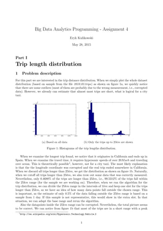
For this part we are interested in the trip distance distribution. When we simply plot the whole dataset
distribution (based on sample from the file 2010 03.trips) as shown on figure 1a, we quickly notice
that there are some outliers (most of them are probably due to the wrong measurement, i.e., corrupted
data). However, we already can estimate that almost most trips are short, what is logical for a city
taxi.
(a) Based on all data (b) Only the trips up to 25km are shown
Figure 1: Histograms of the trip lengths distribution.
When we examine the longest trip found, we notice that it originates in California and ends up in
Spain. When we examine the travel time, it requires hypersonic speeds of over 20Mach and traveling
over ocean. This is theoretically possible1, however, not for a city taxi. The most likely explanation
is that the the longitude coordinate was corrupted and the real trip ended somewhere in California.
When we discard all trips longer than 25km, we get the distribution as shown on figure 1b. Naturally,
when we cutoff all trips longer than 25km, we also trow out some data that was correctly measured.
Nevertheless, only 0.4688% of the trips are longer than 25km, i.e., 99.5312% of the trips fall within
the 25km range (for the sample we are working on). Therefore, when we run the algorithm for the
trip distribution, we can divide the 25km range in the intervals of 1km and keep one slot for the trips
longer than 25km, so we have an idea of how many data points fall outside the chosen range. This
is important, as the estimate of only 0.5% of the data falling outside the 25km range is based on a
sample from 1 day. If this sample is not representative, this would show in the extra slot. In that
situation, we can adapt the base range and rerun the algorithm.
Also the datapoints inside the 25km range can be corrupted. Nevertheless, the total picture seems
to be correct. We can notice from figure 1b that most of the trips are in a short range with a peak
1
http://en.wikipedia.org/wiki/Hypersonic Technology Vehicle 2
1

2. around 2km, and some trips are longer with a peak around 20km. The longer trips could be, for
example, trips to the airport, etc.
2 Implemented algorithms
First implementation that I did was in Matlab. This is very trivial and requires only few lines of
code (see also ex1.m file). Matlab uses an interpreted language, therefore it is not the most optimal
implementation that can be done. Nevertheless, it is very efficient, since the data fits in the memory.
The whole algorithm needs only little bit over 1s (1.32s) to complete, and this includes reading the
data and plotting the figure. Nevertheless, when we run the algorithm after a fresh start of the Matlab,
this also requires loading some libraries with the first run of the algorithm, and the running time is
around 2.43s. It would be more fair to compere this running time with the local running time of the
Hadoop code, as it also requires loading libraries, starting the virtual machine, etc. Note that starting
Matlab takes 7 to 8 seconds.
Hadoop implementation is straight forward as we simply count the trips within an interval. It is not
much different from the WordCount examples as can be found in the Hadoop tutorial, except for using
the String.split(string) instead of StringTokenizer, which is legacy code. For the distance calculations
I have used the spherical Earth projected to a plane flat-surface formula. Following the reasoning
described in section 1, I have decided to add a threshold value as a parameter. That value is then the
upper-bound for the trip length and the trips longer than the threshold are not included in the results
(if we do not pass this parameter, no threshold is used, i.e., this value is set to Integer.MAX VALUE,
and all trips are counted in the results). Nevertheless, the trips that fall outside of this threshold are
counted with an Hadoop Counter and are displayed on the terminal with other counters (and can also
be found in the logs). The results contain then the counts for each 1km interval lower than or equal
the threshold value. For example, when we run the algorithm with threshold 25, we see this output in
the terminal:
Listing 1:
Threshold : 25
Wrong format r e c o r s : 0
Map input records : 441933
Above threshold : 2072 , 0.47% of t o t a l records ( excluded from r e s u l t s )
Zero distance : 7460 , 1.69% of t o t a l records ( included in [ 0 , 1 ] i n t e r v a l )
The output of the algorithm contains a number representing the interval (1 represents the [0, 1]
interval, 2 represents the (1, 2] interval, 3 represents the (2, 3] interval, etc.) and the corresponding
count of the trips that fall within that interval. For the threshold value 25, we would have exactly
25 counts in the output. For more details on the code, see the code itself (TripDist.java, it is really
straight forward).
When run locally, Hadoop reports 0ms CPU time and 81ms garbage collection time. Nevertheless,
the total running time is 3.22s, i.e., very comparable with the Matlab algorithm. Hadoop introduces
overhead of serializing intermediary results and transferring serialized data between the components,
sorting and synchronization code, loading the components in the containers, etc., so it is expected
that the running time would be slightly longer. Also, we need only one Map, we use the Combine step
(that actually does all the work since all data passes in this case by the Combiner in one pass, Reducer
simply outputs the results here and we can even skip it for better efficiency, however no time difference
could be measured locally as we only pass 25 records to the reducer) and the data fits in memory,
making the time very comparable. The result is exactly the same as the one obtained with Matlab and
the plot of the histogram is also exactly the same (see also figure 2 and the ex1.m that contains the
plotting code for Matlab). When we run the code on the cluster, we have additional network latency,
etc., so the running time is expected to be longer than what is observed locally. When run on cluster,
the code needed 20.339s to finish. This is also understandable. Note that we use only one Map, as the
Hadoop documentation mentions, setting up a Map task takes a while and each Map task should take
at least one minute in order to be efficient. It is clear that for this small dataset, it is better to run
the code locally.
2

3. Figure 2: Plot of the result from Hadoop with threshold set to 25.
Part II
Top-k detours
3 Problem description
In this part we are interested in the top-k trips with highest detour ratio. We define the detour ratio
as the total trip length divided by the distance between the two end points of the trip. This ratio
would be infinite for trips with the distance between the two end points of the trip equal to zero and
the non-zero total trip length. From the previous exercise we know that there are many trips with zero
end-to-end distance in the data, approximately 1.69%, because of an error in the data, or, this trips
could be legitimate. This could happen, for example, when a tourist wants to see the city and then get
back to his/hers hotel. An other scenario could be that a person goes somewhere, lets the taxi wait,
and returns to an original location. In all of these cases we cannot really call these trips detours, as
the start and the end point are effectively the same location with non-zero total length. The same is
true for very short trips, as the passenger could be picked up and dropped on slightly different spot
(e.g., on the other side of the street, etc.). Therefore, also for this part we use a threshold value, but
now for the minimal end-to-end trip distance (the default if 0.5km, about 5min walking distance, or
two city blocks). If no threshold parameter is passed, or is equal to zero, the trips that have infinite
ratio are defined as having Double.MAX VALUE ratio. If both distances are zero (e.g., the passenger
changed his/hers mind), the ratio is 1. The trips with distance below the threshold value are defined
as having ratio −1 (this trips should not show up in the results, unless the minimum trip distance
threshold is set very high and there are not enough trips above the threshold distance, therefore, the
negative value is chosen to indicate that these trips are not valid according to the threshold value).
We are interested in the top-k trips with highest detour ratio. However, returning exactly k results
requires computing all ratios, sorting them, and returning only the first k results. Alternatively, we
could use something like the MinMaxPriorityQueue (or simply the java.util.PriorityQueue). For the
priority queue type of solution we store the top-k trips seen so far in an object or a file accessible by
all reducers, and each reducer after processing a trip checks if the trip has higher ratio than the trip
with the lowest ratio in the queue. If it is the case, the trip is inserted in the queue, while the trip
with the lowest ratio is then removed. Note that we cannot use a java object as queue, as we run on
multiple machines. We could use then a HDFS file, but this requires some locking mechanism (this is
not standard present in the HDFS file system). The best option would be then to use an SQL server
and store the top-k trips there (or simply put a lock to the file in the database, while keeping the
priority queue on a file). However, all jobs would be dependent on a single resource, in the worst case,
running longer than one single job would need.
The post-processing is then a better option. If we want to use job chaining for that, we can use only
one top-k reducer. For example, we could have multiple trip ratio reducers, each resulting in the top-k
trips seen locally for better efficiency (after the combiner step, which could also be optimized to return
only top-k trips), and one top-k reducer that selects then top-k trips from the output from all trip
3

4. ratio reducers. However, when we already select only top-k trips in each ratio reducer, we have only
k∗number reducers results after the first job (in the final code it is k∗number reducers∗number taxis,
since we group by taxi ID). The number of reducers is usually small (e.g., 0.95 * [no. of nodes] * [no.
of maximum containers per node]) and using hadoop map-reduce for processing the final result would
be unnecessary. It would be way more efficient to simply run a script or a local program for that
(Matlab, Perl, Java, or any other), as seen in the the first part of this assignment on a small dataset.
Alternatively, we could approximate the k by choosing a threshold value for the minimal ratio that
we want in our results. By first checking the distribution of the ratios (first map-reduce job), we can
estimate that minimal ratio for the desired k by looking at that distribution. We can then also use
two threshold values for the ratio, minimum and maximum, giving us the results in a specific range
(this could be useful in some cases). This way, we do not need the priority queue or sorting by ratio.
However, since in practice we group by taxi ID, we would still need to post-process the data in order
to construct the final top k results. This also means that we either would have to use the threshold
values for the ratio and approximate the k, or return exactly k results with sorting or using the priority
queue. Also, we still have the problem of approximating the distribution of trip ratios. This cannot
be easily done on a sample, since we need to reconstruct the trips first (i.e., we need a sample of the
trips, not of the individual records), and thus we need to run another job for that.
Therefore, for this assignment, I have chosen the option of selecting the top k solutions locally in
the combiners and reducers. Note that this is done using the priority queue and is only very efficient
(especially for the memory usage) when the k value is much lower than the number of trips (what
should always be the case for this assignment). After that the map-reduce job is ready, the results are
post-processed in the same Java program. Thus, you need to run only one main, the final results are
placed in the result.txt file in the output directory (i.e., in the hadoop file system together with the
output of the individual reducers).
4 Implemented algorithms
This section discusses the various aspects of the implementation of the different components; the
Mapper, the Combiner, and the Reducer.
4.1 Mapper
The input for the map function is a single record. We can not construct the trips on this level, but we
can filter some of the records that have errors, are not correctly formatted, etc.:
• We verify if the record has 9 fields.
• We verify if the taxi ID is a positive integer.
• We verify if the timestamps of the start and the end points fall within the dataset time-frame:
from May 2008 to January 2011. For that, we need to parse the timestamps to the Date objects.
When we do that, we can convert the date to the number of seconds since January 1, 1970,
00:00:00 GMT represented by that Date object, before emitting the record to the combiner, for
easier processing later.
• We verify if the start and end point coordinates are within certain limits (e.g., they are not
in Spain). The default bounding box is within California: latitude 32.32N to 42N, longitude
−114.8E to −124.26E. This can be changed with corresponding parameters (see also the readme
file).
• We verify if the start and end point status is either E or M.
• We calculate the traveling speed, if it is above 200km/h (this s can be set with an argument to
the main), we drop that record. Since we need to calculate the traveled distance for that, we
store the calculated distance for the records with status M,M (i.e., start and end point with
status M ), so we do not need to recalculate it later on.
4

5. • The start time must be before the end time of the segment.
• Finally, a threshold value is used for a segment duration. If a segment is longer than the threshold
value, it is dropped.
For the statistics after running the code, we keep the count of the records that we filter out with
the hadoop counters (one counter for each type of validity check).
After filtering, we emit the records with as composite key a Text containing the taxi ID (we group
by taxi ID) and the start time of the segment (we sort by the start time, i.e., the code uses the
secondary sort feature of hadoop). The records can contain 8 comma separated fields in a Text value
(we use sparse notation, and the data that is not used later is not passed, e.g., for empty records
(i.e., records with status EE) we only need the start and end time, or even better, we drop the empty
records, see also the combiner and reducer sections):
• All of the original fields, except for the taxi ID.
• We merge the status of the start and end point into one segment status (i.e., EE, MM, etc.)
and we encode it as an integer (we have four possible combinations of the start and end status,
combined status is then a number between 0 and 3, see the code for specifics).
• The transformed timestamps to the number of seconds since January 1, 1970, 00:00:00 GMT.
• The distance traveled in the single segment (only for MM segments)
4.2 Combiner
Before the data gets to the combiner, it is grouped by the taxi ID and sorted by the start time by
hadoop. However, as the hadoop documentation mentions, there is no guarantee of the combiner sort
being stable in any sense, as the order of available map-outputs to the combiner is non-deterministic.
In practice, at least for this assignment, it turns out to work quite well and we can already merge
many segments in order to reduce the number of records being passed to the reducers.
The sorting itself is done with the secondary sort of hadoop. This is quite straight-forward as
there are many tutorials available online. We need to use composite keys (in this case, the taxi ID for
grouping and the start time of the segment for sorting), implement two comparators (one for sorting
and one for grouping, see also the TaxiTimeSortComparator and TaxiTimeGroupingComparator in
the code) and the custom partitioner (TaxiTimePartitioner in this case). Implementation of these
classes is very straight forward. Also the usage is very easy, as we only need few lines of code to
configure the job correctly.
Since there is no guarantee of the secondary sort at the combiner level, we can only make best
effort to merge some of the records. For example, we can merge subsequent empty records into one
record, etc. The most important for this assignment are the trips. A valid trip usually starts with an
EM segment, followed by MM segments, and it ends with en ME segment. As we read quite a lot of
data with each mapper (the default is 128MB), there is a good chance that we will merge many trips
at the combiner level. As an optimization, the combiner returns only the top-K highest ratio trips it
finds.
The chosen technique for that is the priority queue. For that purpose, the trips are stored in a
custom Comparable object, where the values that are compared are the ratios (see the RatioTripPair
class). These custom objects are then stored in a priority queue (java.util.PriorityQueue) with initial
capacity k + 1. When the queue holds k objects and one more trip is constructed, that trip is first
added to the queue, and the trip with the lowest detour ratio is then removed. This way, the queue
holds at most k trips with the highest ratios seen so far. After that the combiner is done, at most k
trips are returned in the results.
The merging of the segments is a more complicated process. Since we are not certain about the
secondary sort of hadoop at the combiner level (as discussed earlier), we need to be careful which
records we merge. The chosen strategy is to merge two subsequent records only if the first one has the
same end time as the start time of the second record. Additionally, also the check on the coordinates
5

6. could be implemented, but it seemed not needed, as the correct measurements are redundant, i.e., the
end of one segment is exactly the same as the start of the next and it would only slow down the code.
Nevertheless, this is trivial and can be easily added. The merging itself is organized as follows:
• First we check if the current segment does not start before the previous one ended. If this is not
true, we drop the current segment. We know that both segments, previous and current, have
a valid duration according to the chosen threshold value, i.e., we could drop any of the two
segments to resolve the conflict. However, choosing the current one significantly simplifies the
code. Otherwise, we would have to unmerge some records, or iterate over the segments more
than once, etc.
• Empty records (EE) can be only merged with other empty records. Ideally, the mapper does not
emit empty records, and no empty records can be found at the combiner level. However, this has
a risk at the reducer level. The empty records help to distinguish between two different trips.
For example, the mapper already drops many records that do not pass the validity checks, and
if unlucky, we drop the ME and EM records making it harder to clearly distinguish between
two trips. By default, no empty records are emitted. Nevertheless, this can be changed with the
corresponding argument.
• Ideally, the other merged records would be all trips. However, because we can only make the best
effort at merging the trips, we can end up with trip parts (e.g., EM-MM-MM, MM-MM, etc.).
We can simplify some cases, e.g., when we merge two MM records, the result is an MM record.
Nevertheless, the total number of possible states is 7 (i.e., extra three states to the original four).
The newly defined states are EMMM, MMME, and EM(MM)ME (a full trip). These merged
segments are then the input to the reducer.
• The reconstructed trips have a detour ratio. These ratios are then also stored in the trip records.
The output of the combiner is then a collection of trips, partially reconstructed trips and possibly
empty records (segments with status EE). As mentioned earlier, the empty records can be already
filtered out at the mapper level by setting the corresponding argument. Each combiner can emit at
most k reconstructed trips. Since we group by taxi ID, we can have at most k ∗ NbCombiners ∗
NbTaxiIDs reconstructed trips at this point. Additionally, the reducer will reconstruct many trips
from the remaining (merged) segments.
4.3 Reducer
The reducer is almost exactly the same as the combiner. Except, it makes greater effort at recon-
structing the trips and outputs only the reconstructed trips.
The effort of reconstructing the trips is regulated with the maximum time gap between the records.
By default, the maximum duration of a segment is two minutes and the maximum gap between two
records is 90s. These values are chosen such that we are very certain about the reconstructed trips
(if we want to decide that some trips are illegitimate, we should be certain about the data quality
first). Usually, the segments span one minute. We take two minutes as the maximum, such that most
of the correct segments will not be filtered out (we prefer to keep the data than trying to reconstruct
it later). The rather low setting for the maximum time gap is sufficient to merge two segments where
in between one segment of 90s is missing (i.e., longer than representative 1 minute, but shorter than
two segments of 1 minute each). In other words, in most cases, we can reconstruct one segment, given
that the we have the two neighbor segments. The reasoning behind it is that when more than one
subsequent segments are missing, there is a significant portion of a trip that we are uncertain about,
and the quality of the reconstruction suffers.
Reconstructing only one segment especially helps in situations where, for example, we would merge
two trips into one because the two segments that are missing are the ME and EM segments. We still
run that risk, but it is lowered. In fact, these values permit to safely drop the empty records at the
mapper level, making the code very efficient. Also, we have many trips in the data, missing some of
them (actually all trips of non-trivial length are in the results, only some trips are split in more than
6

7. one trip when this strategy is followed because of the reconstruction difficulties) does not influence
the end results greatly. For the best possible accuracy, we can still change the parameter values. For
example, we could emit the empty records at the mapper and than use the maximum time gap larger
than the maximal segment duration, etc.
The output of the reducer is then a collection of trips. We group by taxi ID, so we have k ∗
NbReducers∗NbTaxiIDs trips, unsorted. The class TopKFinalResult is then used for final processing.
It was easiest to do that from java code, as we can easily access the hadoop file system. In the final
processing, the results are sorted by the ratio (with highest ratios on top) and only the top-k results
are returned (the same algorithm with the priority queue is used as in the combiner and the reducer).
Also, the timestamps of the trip start and end are reconstructed for easier reading. Because the output
of the reducer is small, the post-processing does not take significant amount of time (it is negligible
when compared to the running time of the map-reduce).
Finally, because in the end result we do not have intermediary coordinates of the trip (only the
trip start and the trip end are returned), an additional map-reducer class is implemented, see the
GetTrip.java. We can then use this to start a second job (with the same jar, see the readme file) to
retrieve the segments from the data for a specific trip we are interested in. The implementation of this
is very simple, as only the mapper is used (no combiner or reducer). It iterates over all records and
filters only the relevant ones. A simple post-processing (GetTripFinalResult) is used to sort the results
by starting time, output the coordinates separately from the segments for easy viewing on the map
service, etc. The segments are also included in the results for debugging purposes. Also the counters
are used as in the detour implementation for debugging information.
5 Performance and results
The implemented code scales very well without additional improvements. For example, on the large
dataset on the cluster, the job needs around 15 to 16 minutes (depending on the conditions) to complete
for k = 100. For comparison, the second job to retrieve the intermediary coordinates of a specific trip
needs almost 14 minutes. The second job is trivial, as it only filters few data points and uses only
mappers. Basically, it is limited by the disk IO and does almost no computations (also no records are
send to reducers, etc.) and thus it sets the limit to what can be expected in terms of performance.
One idea that I wanted to try (out of curiosity) was to implement a single top-k reducer. I thought
I could skip the detour combiner and use the detour reducer instead. This way, only the trip records
would be returned at the combiner level, with loss of accuracy (as discussed earlier, we do not have
any guarantee on the records that we get on the combiner level, and they are certainly not complete
for any taxi ID when large dataset is used). However, this approach failed because of the sorting
and partitioning problem and the possibly low quality of the results when compared to the original
implementation.
The code for the top-k reducer does not run on the cluster, I think it is because I can only set
one partitioner and one sorting comparator (I can set different grouping comparators for the combiner
and the reducer (for the top-k reducer it is trivial, where all objects are equal), but this option is
not available for the other components). The code probably crashes then on keys that are no longer
composite of taxi ID and the start time (the error is very unclear). This could be fixed, but the
only clean way to do it is to set a separate job. However, as discussed earlier (and observed from the
experiments), it is more efficient to post-process the small data with a regular Java class than to force a
map-reducer on it. Nevertheless, when I run the code locally on the small dataset (taxi 706.segments),
the code does not crash, but no gain in performance can be observed (as discussed earlier, the original
code gets already close to the limit set by the simple GetTrip implementation), making this approach
very uninteresting.
As for the number of reducers, I have tried using the formula 0.95 * [no. of nodes] * [no. of
maximum containers per node]. With 4 containers per node, we would have around 34 reducers.
Nevertheless, the setting closer to the number of nodes worked better, and I have executed most of
my jobs with 8 reducers. For the file split size, the standard setting of 128MB works also very well.
As it turns out, it is not easy to find illegitimate detours. When I use the minimum end-to-end
7

8. distance of only 0.5km, the trips that I find are usually indicating that the start point end end point
are the same. For example, one trip that I have found is from the airport to a private home, after two
minutes, the taxi rides back to the airport (the client probably forgot his passport). It is usually more
interesting to set the minimum end-to-end distance higher.
Even with higher setting it is not guaranteed to find illegitimate trips. For example, the trip with
highest detour ratio in the large data set with this value set to 10km shows that a person (a priest?)
goes to one church, lets the taxi wait for an hour (from 9 to 10 in the morning) and then goes to
another church. It is then more likely that illegitimate tours have also lower ratio and will not necessary
show in the first few hits with extremely high ratios.
The best strategy was to get more candidate tours (e.g., top 100), and look for recurrent taxi ID.
This might indicate that a particular driver is more likely to have illegitimate tours. For example, with
this strategy I have found one trip that seems illegitimate to me: on the way to the airport, the driver
took the wrong highway, and only after quite a long distance he turned around to get to the airport,
but did not turn off the meter. This trip is shown on figure 3. More in general, even by manually
looking at the trips, it is not easy to tell if the trips are legitimate or not. In the case described above,
they might have picked up another person that was waiting next to the exit, etc.
Figure 3: Illegitimate detour candidate.
8