Unit 4 external sorting

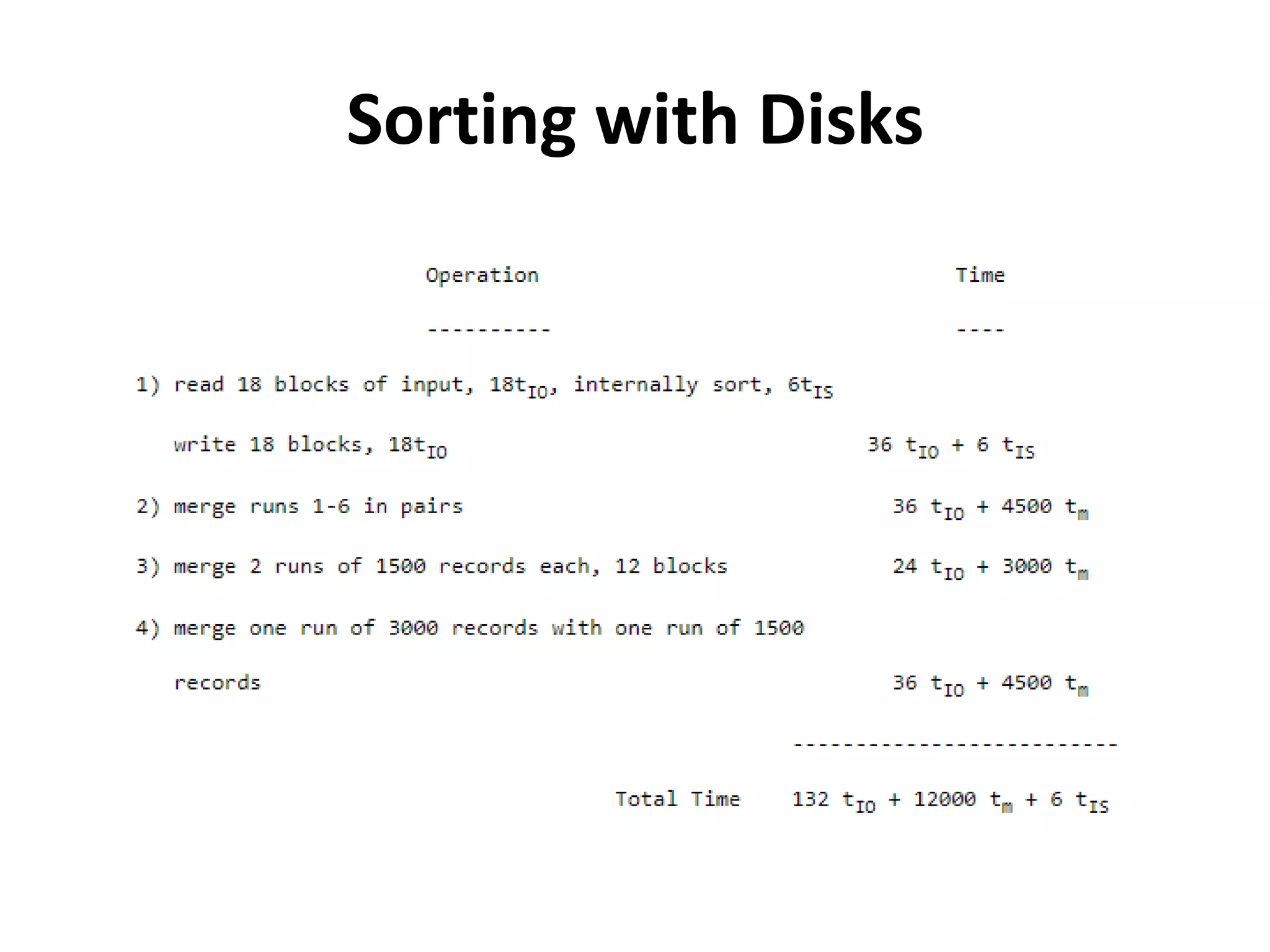
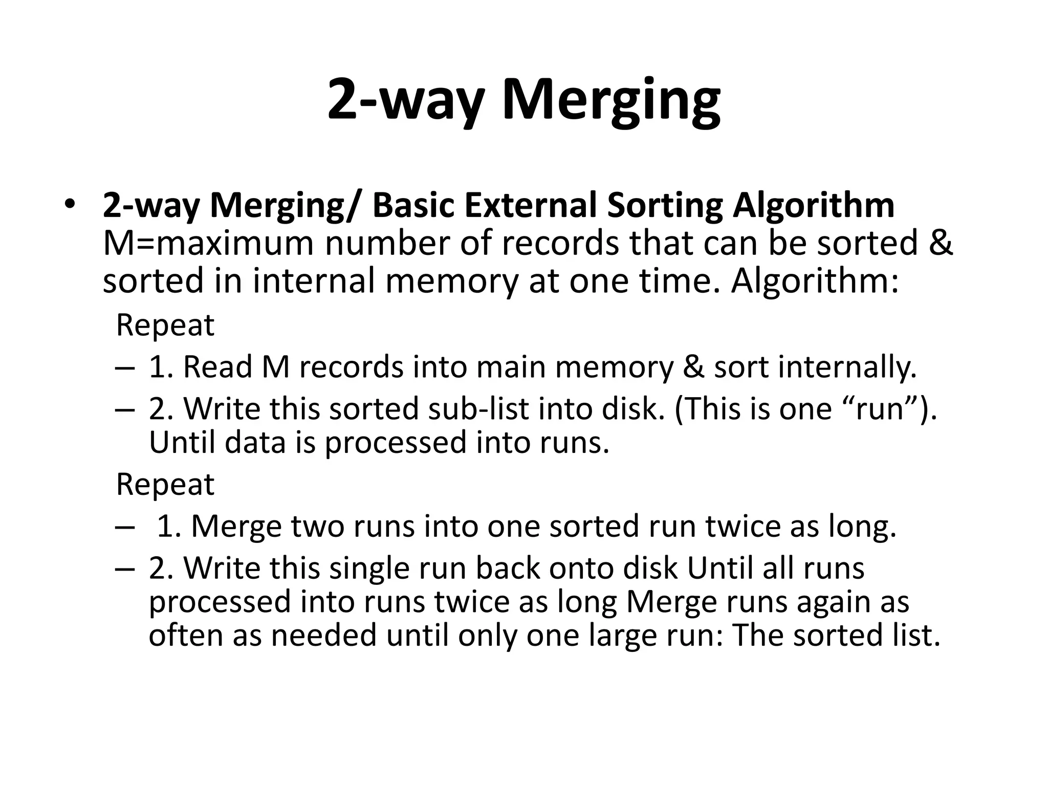
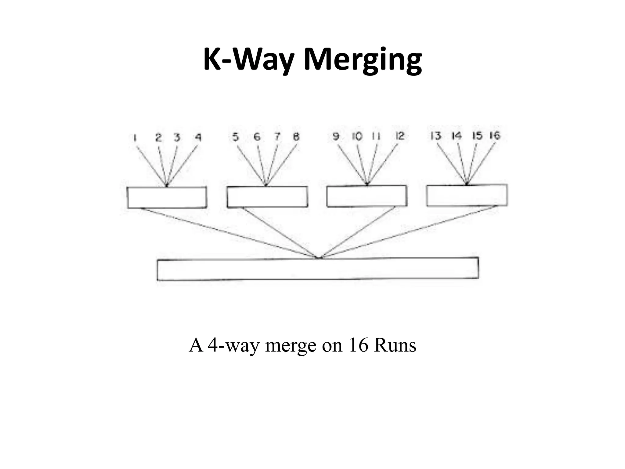
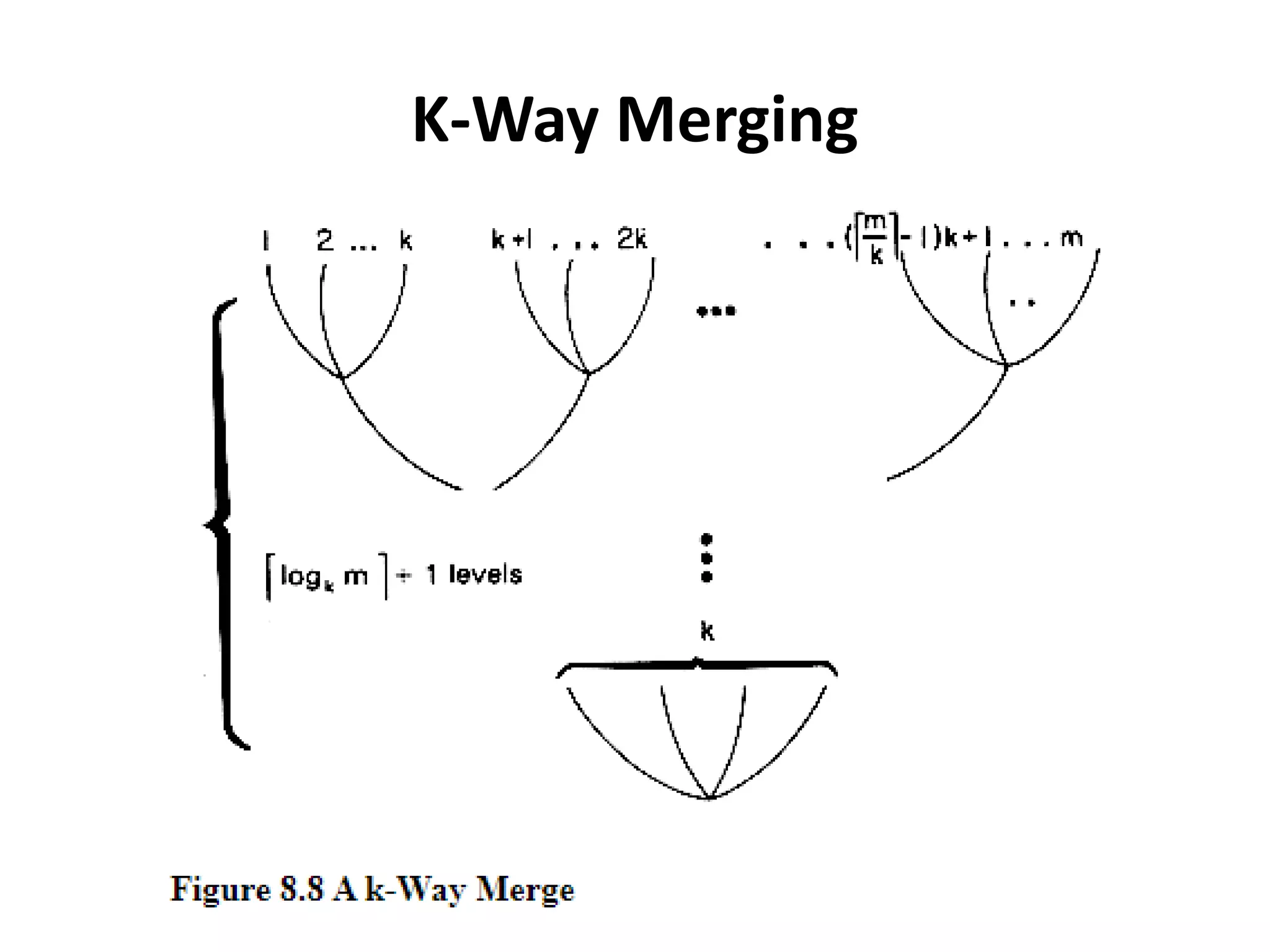
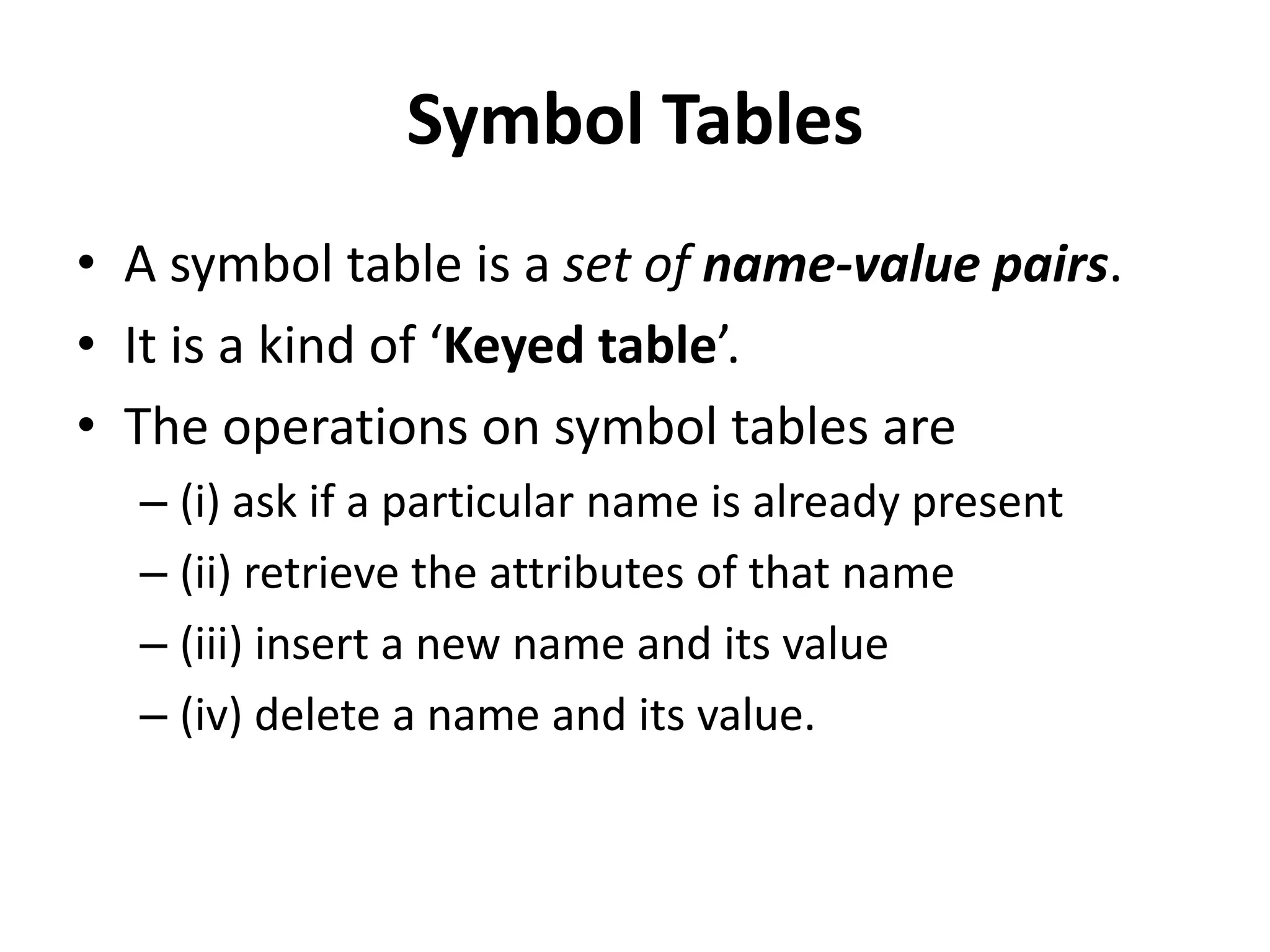
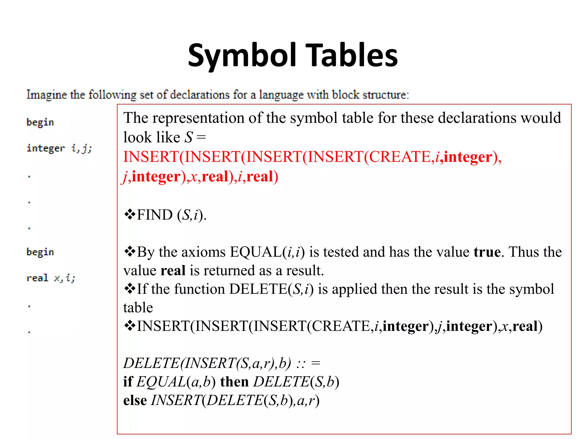
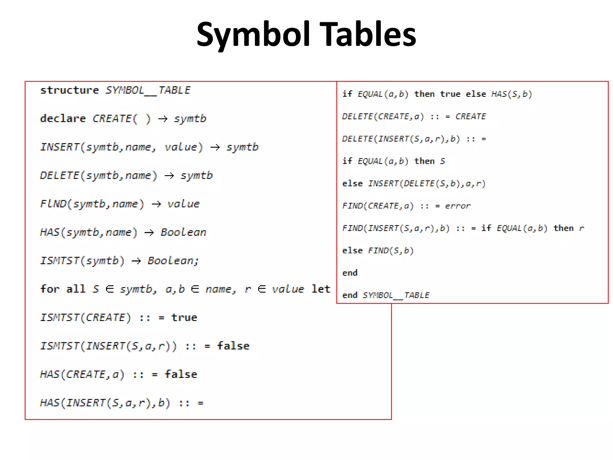
Unit 4
External Sorting & Symbol Tables
Dr. R. Khanchana
Assistant Professor
Department of Computer Science
Sri Ramakrishna College of Arts and Science for
Women
http://icodeguru.com/vc/10book/books/book1/chap08.htm
http://icodeguru.com/vc/10book/books/book1/chap09.htm

Storage Devices
Magnetic Tapes
Disk Storage

Magnetic Tapes
• Magnetic tape devices are similar
in principle to audio tape
recorders.
• The data is recorded on magnetic
tape approximately 1/2" wide.
• The tape is wound around a spool.
• A new reel of tape is normally
2400 ft. long.
• Tracks run across the length of the
tape, with a tape having typically
7 to 9 tracks across its width.

Magnetic Tapes
• Depending on the direction of magnetization, a
spot on the track can represent either a 0 or a 1
(i.e., a bit of information).
• The combination of bits on the tracks represents
a character (e.g., A-Z, 0-9, +, :, ;, etc.).
• The number of bits that can be written per inch
of track is referred to as the tape density.
• Standard track densities are 800 and 1600 bpi
(bits per inch).

Magnetic Tapes
• The code for the first
character on the tape is
10010111 while that
for the third character
is 00011100.
• If the tape is written
using a density of 800
bpi then the length
marked x in the figure
is 3/800 inches.

Magnetic Tapes
• A tape drive consists of two
spindles.
• On one of the spindles is mounted
the source reel and on the other
the take up reel.
• During forward reading or forward
writing, the tape is pulled from the
source reel across the read/write
heads and onto the take up reel.
• Some tape drives also permit
backward reading and writing of
tapes; i.e., reading and writing can
take place when tape is being
moved from the take up to the
source reel.

Magnetic Tapes
• If characters are packed onto a tape at a density of 800 bpi, then a
2400 ft. tape would hold a little over 23 x 106 characters.
• A density of 1600 bpi would double.
• The information on a tape will be grouped into several blocks.
• These blocks may be of a variable or fixed size.
• In between blocks of data is an interblock gap normally about 3/4
inches long.
• The interblock gap is long
enough to permit the tape to
accelerate from rest to the
correct read/write speed before
the beginning of the next block
reaches the read/write heads.

Magnetic Tapes
• The block of data is packed into the words A, A +
1, A + 2, .... Similarly, in order to write a block of
data onto tape one specifies the starting address
in memory and the number of consecutive
words to be written. These input and output
areas in memory will be referred to as buffers.
• Usually the block size will correspond to the size
of the input/output buffers set up in memory.

Magnetic Tapes
• The blocks to be as large as possible for the following reasons:
• (i) Between any pair of blocks there is an interblock gap of 3/4".
– With a track density of 800 bpi, this space is long
enough to write 600 characters.
– Using a block length of 1 character/block on a 2400
ft. tape would result in roughly 38,336 blocks or a
total of 38,336 characters on the entire tape.
– Tape utilization is 1/601 < 0.17%. With 600
characters per block, half the tape would be made
up of interblock gaps.

Magnetic Tapes
• (ii) If the tape starts from rest when the input/output command
is issued, then the time required to write a block of n characters
onto the tape is ta + ntw where ta is the delay time and tw the
time to transmit one character from memory to tape.
– The delay time is the time needed to cross the interblock
gap.
– Assuming a tape speed of 150 inches per second during
read/write and 800 bpi the time to read or write a character
is 8.3 x 10-6sec.

Magnetic Tapes
• If the entire tape consisted of just
one long block, then it could be
read in
• An average transmission rate of almost 12 x 104 charac/sec.
• The tape would have at most 38,336 characters or blocks.
• This would be the worst case and the read time would be
about 6 min 24 sec or an average of 100 charac/sec.
• In this case the time to read 38,336 one character blocks
would be 3 min 12 sec, corresponding to an average of about
200 charac/sec.

Magnetic Tapes
Assumptions about tape drives:
(i) Tapes can be written and read in the forward direction only.
(ii) The input/output channel of the computer is such as to
permit the following three tasks to be carried out in parallel:
- Writing onto one tape
- Reading from another and
- CPU operation
(iii) If blocks 1, ...,i have been written on a tape, then the tape
can be moved backwards block by block using a backspace
command or moved to the first block via a rewind command.

Disk Storage
• Direct access external storage
• Two distinct components:
– Disk module (or simply disk or disk pack) on which
information is stored (this corresponds to a reel of
tape)
– Disk drive (corresponding to the tape drive) which
performs the function of reading and writing
information onto disks.

Disk Storage
• Figure 8.4 shows a disk pack with 6 platters.
• Each platter has two surfaces on which information can be recorded.
• The outer surfaces of the top and bottom platters are not used. This
gives the disk of figure 8.4 a total of 10 surfaces on which information
may be recorded.
• A disk drive consists of a spindle on which a disk may be mounted and
a set of read/write heads.
• There is one read/write head for each surface. During a read/write the
heads are held stationary over the position of the platter where the
read/write is to be performed, while the disk itself rotates at high
speeds (speeds of 2000-3000 rpm are fairly common).
• Device will read/write in concentric circles on each surface. The area
that can be read from or written onto by a single stationary head is
referred to as a track.
• Tracks are thus concentric circles, and each time the disk completes a
revolution an entire track passes a read/write head. There may be
from 100 to 1000 tracks on each surface of a platter.
• The collection of tracks simultaneously under a read/write head on the
surfaces of all the platters is called a cylinder.
• Tracks are divided into sectors. A sector is the smallest addressable
segment of a track. Information is recorded along the tracks of a
surface in blocks

Disk Storage
• Three factors contributing to input/output time
for disks:
• (i) Seek time: time taken to position the read/
write heads to the correct cylinder. This will
depend on the number of cylinders across which
the heads have to move.
• (ii) Latency time: time until the right sector of the
track is under the read/write head.
• (iii) Transmission time: time to transmit the block
of data to/from the disk.

Disk Storage
• Maximum seek times on a disk are around 1/10 sec.
• A typical revolution speed for disks is 2400 rpm.
• Hence the latency time is at most 1/40 sec (the time
for one revolution of the disk).
• Transmission rates are typically between
105 characters/second and 5 x 105 characters/second.
• The number of characters that can be written onto a
disk depends on the number of surfaces and tracks per
surface.
• This figure ranges from about 107 characters for small
disks to about 5 x 108 characters for a large disk.

Sorting with Disks
K –way Merging

Sorting with Disks
• The most popular method for sorting on external storage devices is merge
sort.
• This method consists of essentially two distinct phases.
• First, segments of the input file are sorted using a good internal sort
method.
– These sorted segments, known as runs, are written out onto external storage as they
are generated.
• Second, the runs generated in phase one are merged together following
the merge tree patter until only one run is left

Sorting with Disks
• Analyze the method described above to see how much
time is required to sort these 4500 records. The
analysis will use the following notation:
• ts = maximum seek time
• tl = maximum latency time
• trw = time to read or write one block of 250 records
• tIO = ts + tl + trw
• tIS = time to internally sort 750 records
• n tm = time to merge n records from input buffers to
the output buffer

2-way Merging
• 2-way Merging/ Basic External Sorting Algorithm
M=maximum number of records that can be sorted &
sorted in internal memory at one time. Algorithm:
Repeat
– 1. Read M records into main memory & sort internally.
– 2. Write this sorted sub-list into disk. (This is one “run”).
Until data is processed into runs.
Repeat
– 1. Merge two runs into one sorted run twice as long.
– 2. Write this single run back onto disk Until all runs
processed into runs twice as long Merge runs again as
often as needed until only one large run: The sorted list.

K-Way Merging
A 4-way merge on 16 Runs

Sorting with Tapes
Balanced Merge Sort
Polyphase Merge

Polyphase Merge
A polyphase merge sort is a variation of bottom up Merge sort that sorts a list
using an initial uneven distribution of sub-lists, primarily used for external
sorting, and is more efficient than an ordinary merge sort when there are fewer
than 8 external working files. A polyphase merge sort is not a stable sort.

Symbol Tables
• A symbol table is a set of name-value pairs.
• It is a kind of ‘Keyed table’.
• The operations on symbol tables are
– (i) ask if a particular name is already present
– (ii) retrieve the attributes of that name
– (iii) insert a new name and its value
– (iv) delete a name and its value.

Symbol Tables
The representation of the symbol table for these declarations would
look like S =
INSERT(INSERT(INSERT(INSERT(CREATE,i,integer),
j,integer),x,real),i,real)
FIND (S,i).
By the axioms EQUAL(i,i) is tested and has the value true. Thus the
value real is returned as a result.
If the function DELETE(S,i) is applied then the result is the symbol
table
INSERT(INSERT(INSERT(CREATE,i,integer),j,integer),x,real)
DELETE(INSERT(S,a,r),b) :: =
if EQUAL(a,b) then DELETE(S,b)
else INSERT(DELETE(S,b),a,r)

Representation of Symbol Tables
• There are two different techniques for implementing a
keyed table
– Static Tree Tables
• It is used when symbols are known in advance and no
insertion and deletion is allowed
– Dynamic Tree Tables
• It is used when symbols are not known in advance but
are inserted as they come and deleted if not required
– Hash Tables
• Hash tables are created with an algorithm that stores the
keys into hash buckets, which contain key-value pairs.

9.1 STATIC TREE TABLES
• Definition: A binary search tree T is a binary
tree; either it is empty or each node in the
tree contains an identifier and:
(i) all identifiers in the left subtree of T are less (numerically or
alphabetically) than the identifier in the root node T;
(ii) all identifiers in the right subtree of T are greater than the
identifier in the root node T;
(iii) the left and right subtrees of T are also binary search trees.

Extended Binary Tree
•N Nodes ( Internal Nodes)
•N+1 Null Links (Square Nodes
–External Nodes- not part of
the original Tree)

Internal vs External Path length
• Internal length Path
The sum over all internal nodes of the lengths of
the paths from the root to those nodes.
• External length Path
• The sum over all external nodes of the lengths of
the paths from the root to those nodes.

Internal vs External Path length

• Internal Path Length
• At most 2 nodes at distance 1, 4 at distance 2,
and in general the smallest value for I is
• 0 + 2 1 + 4 2 + 8 3 + ....
• This can be more compactly written as

• For example, suppose n = 3 and we are given the
four weights: q1 = 15, q2 = 2, q3 = 4 and q4 = 5.
• Two possible trees would be:
• Their respective weighted
external path lengths are:

Huffman Code
• Huffman coding is a lossless data compression algorithm.
• In this algorithm, a variable-length code is assigned to input
different characters.
• The binary bits in the code word for a message determine the
branching needed at each level of the decode tree to reach
the correct external node.
• For example, If we interpret a zero as a left branch
and a one as a right branch, then the decode tree
corresponds to codes 000, 001, 01 and 1
for messages M1, M2, M3 and M4 respectively.
These codes are called Huffman codes.

Assignment
Binary Tree Construction

Test data
• To test it to determine whether or not it is
doing the right thing. Here is a sequence of
random integers:

Random integers
• 41 67 34 0 69 24 78 58 62 64 5 45 81 27 61 91
95 42 27 36 91 4 2 53 92 82 21 16 18 95 47 26
71 38 69 12 67 99 35 94 3 11 22 33 73 64 41
11 53 68

Assignment
• Construct Binary Tree for the Months of the
Year…
– Binary Tree
– Skewed Binary Tree

Assignment Results
Binary Search Tree

Assignment Results
Binary Search Tree(Right -Skewed)
Figure 9.9 Degenerate binary
search tree

Height Balanced Binary Trees
(AVL Trees)
• A binary tree is height balanced provided both the left and
right sub trees are height balanced and the heights of the left
and right sub tress differ by at most one.
• Definition: An empty tree is height balanced. If T is
a nonempty binary tree with TL and TR as its left and
right subtrees, then T is height balanced iff
– (i) TL and TR are height balanced and
– (ii) |hL - hR| <= 1 where hL and hR are the heights
of TL and TR respectively.

Height Balanced Binary Trees
(AVL Trees)

AVL Trees
• Definition: The balance factor, BF(T), of a node T in
a binary tree is defined to be hL -hR where hL and hR are
the heights of the left and right subtrees of T.
• For any node T in an AVL tree BF(T) = - 1, 0 or 1.

AVL Trees
• To balance the tree the following characterization of
rotation types is obtained:
• LL: new node Y is inserted in the left subtree of the left subtree
of A
– Anti-clockwise Rotation
• LR: Y is inserted in the right subtree of the left subtree of A
• RR: Y is inserted in the right subtree of the right subtree of A
– Clockwise Rotation
• RL: Y is inserted in the left subtree of the right subtree of A

Double Rotation
Left –Right Rotation
Right –Left Rotation

Assignment
• General Quiz
https://quizizz.com/admin/quiz/5f6c30200a2303001ec13a9c
• Workout the AVL Trees
– Input Order
• Mar, May, Nov, Aug, April, Jan, Dec, July, Feb, June, Oct,
Sep

9.3 Hash Tables
• Hash table HT with b = 26 buckets,
• Each bucket having exactly two slots, i.e., s = 2.
• Assume that there are n = 10 distinct identifiers in
the program and that each identifier begins with
a letter. The loading factor, , for this table is 10/52
= 0.19.
• The hash function f must map each of the
possible identifiers into one of the numbers 1-26.

Hash Tables
• If the internal binary representation for the letters A-Z corresponds to the
numbers 1-26 respectively, then the function f defined by:
• f(X) = the first character of X; will hash all identifiers X into the hash table.
The identifiers GA, D, A, G, L, A2, A1, A3, A4 and E will be hashed into
buckets 7, 4, 1, 7, 12, 1, 1, 1, 1 and 5 respectively by this function.
• The identifiers A, A1, A2, A3 and A4 are synonyms. So also are G and GA

• Is there a data structure where inserting, deleting
and searching for items are more efficient?
• The answer is “Yes”, that is a Hash Table.

9.3.1 Hashing Functions
• A hashing function, f, transforms an identifier X into
a bucket address in the hash table.
• I.e., if X is an identifier chosen at random from the
identifier space, then we want the probability
that f(X) = i to be 1/b for all buckets i. Then a
random X has an equal chance of hashing into any of
the b buckets.
• A hash function satisfying this property will be
termed a uniform hash function.

Hashing -Problems
• Collision:
– It occurs when two non-identical identifiers are
hashed into the same bucket.
• Overflow :
– An overflow is said to occur when a new identifier
I is mapped or hashed by f into a full bucket

Uniform Hash Functions
• Several kinds of uniform hash functions are in
use. We shall describe four of these.
• (i) Mid-Square
• (ii) Division
• (iii) Folding
• (iv) Digit Analysis

Mid-Square
Middle of the Square function
- Function fm is computed by squaring the
identifier and then using an appropriate
number of bits from the middle of the
square to obtain the bucket address.

Division
• Modulo (mod) operator is used to obtain the bucket address
• fD(X) = X mod M
• If M is divisible by 2 then odd keys are mapped to odd
buckets (as remainder is odd) and even keys are
mapped to even buckets

Digit Analysis
• This method is particularly useful in the case
of a static file where all the identifiers in the
table are known in advance.
• Each identifier X is interpreted as a number
using some radix r.
• The same radix is used for all the identifiers in
the table. Using this radix, the digits of each
identifier are examined

Quiz
• https://quizizz.com/admin/quiz/5f76d8ea31
8e91001b21bb8b

Unit 4 external sorting

Recommended

Recommended

More Related Content

What's hot

What's hot (20)

Similar to Unit 4 external sorting

Similar to Unit 4 external sorting (20)

More from DrkhanchanaR

More from DrkhanchanaR (7)

Recently uploaded

Recently uploaded (20)

Unit 4 external sorting

Editor's Notes