SlideShare a Scribd company logo
1 of 49
Download to read offline
APPROACHES TO MODELING OF
REACTIVE TRANSPORT IN POROUS MEDIA
Carl I. Steefel1
Kerry T.B. MacQuarrie2
1
Department of Geology
University of South Florida
Tampa, Florida 33620 U.S.A.
2
Department of Earth Sciences
University of Waterloo
Waterloo, Ontario N2L 3G1 Canada
Reprinted from:
Reactive Transport in Porous Media
(P.C. Lichtner, C.I. Steefel, and E.H. Oelkers, eds.)
Reviews in Mineralogy 34, 83-125.
1 Now at Lawrence Berkeley National Laboratory, Berkeley, CA 94720
2 Now at Department of Civil Engineering, University of New Brunswick, Fredericton, New Brunswick
E3B5A3 Canada
Steefel, C.I. and MacQuarrie, K.T.B. (1996) Approaches to modeling reactive transport in porous
media. In Reactive Transport in Porous Media (P.C. Lichtner, C.I. Steefel, and E.H.
Oelkers, eds.), Rev. Mineral. 34, 83-125.
Chapter 2
APPROACHES TO MODELING OF
REACTIVE TRANSPORT IN POROUS MEDIA
Carl I. Steefel
Department of Geology
University of South Florida
Tampa, Florida 33620 U.S.A.
Kerry T. B. MacQuarrie1
Department of Earth Sciences
University of Waterloo
Waterloo, Ontario N2L 3G1 Canada
INTRODUCTION
Most of the geochemical and biogeochemical phenomena of interest to Earth scientists
are the result of the coupling of some combination of fluid, heat, and solute transport with
chemical reactions in the Earth’s crust. Rather than being isolated systems that can be
described entirely by thermodynamics, environments in the Earth’s crust act as open bio-
geochemical reactors where chemical change is driven by the interactions between migrating
fluids, solid phases, and organisms. These interactions may involve such diverse processes
as mineral dissolution and precipitation, adsorption and desorption, microbial reactions,
and redox transformations. If the interactions take place over sufficiently long periods of
time, they may modify the properties of the porous media itself, for example through the
dissolution of matrix minerals or the cementation of pore spaces.
Because of the complexity of reactive transport processes in porous media, modeling
their dynamic behavior is a challenging task for the geoscientist. The complexity of the
field is in part a natural consequence of the evolution of the scientific disciplines which
contribute to the broader subject of reactive transport in porous media. For example, con-
tinuing research on multicomponent aqueous geochemical systems makes it clear that the
traditional means of modeling transport and reactions in groundwater systems using single
ion approaches do not capture all of the chemical complexities (e.g. pH dependence of
adsorption, nonlinear kinetic reaction rates) which exist in these systems. Research carried
out over the last 10 years has also called into question the time-honored local equilibrium
assumption (Thompson, 1959) which has been applied almost indiscriminantly in meta-
morphic petrology and many other fields in the geosciences (Lindberg and Runnels, 1984;
Bahr and Rubin, 1987; Steefel and Van Cappellen, 1990; Lasaga and Rye, 1993; Steefel
and Lasaga; 1994; Steefel and Lichtner, 1994; McNab and Narasimhan, 1994; McNab and
Narasimhan, 1995; Friedly et al., 1995; Oelkers et al., 1996; Van Cappellen and Wang,
1996). In addition, the research on geochemical kinetics has revealed a wealth of possible
mechanisms and rates by which minerals, organisms, and aqueous species may interact. In
most cases these interactions are nonlinear and therefore require special treatment in order
to incorporate them into mathematical models. Similarly, hydrologists have highlighted
the complexity of natural porous media in recent years, showing clearly that the dynamic
1Now at Department of Civil Engineering, University of New Brunswick, Fredericton, New Brunswick E3B
5A3 Canada
Steefel & MacQuarrie: Approaches to Modeling Reactive Transport
behavior of contaminant systems (and by implication, all geological systems involving reac-
tions between migrating species and a reactive porous media) is strongly dependent on both
physical and chemical heterogeneities present in the system (Dagan, 1989; Gelhar, 1993;
van der Zee and van Riemsdijk, 1987; Garabedian et al., 1988; Valocchi, 1989; Kabala and
Sposito, 1991; Robin et al., 1991; Tompson, 1993; Bosma et al., 1993; Brusseau, 1994;
Cushman et al., 1995; Hu et al., 1995; Simmons et al., 1995; Ginn et al., 1995; Tompson et
al., 1996; Tompson and Jackson, this volume). The homogeneous porous media assumed
by the classic geochemical reaction path, for example, has limited applicability to natural
porous media. For these reasons, and facilitated by more powerful computer hardware and
advanced numerical methods, the development and application of reactive transport models
has accelerated in the past decade.
It is important to recognize that the numerical methods and the potential errors as-
sociated with these methods follow to some extent from the process formulations. For
example, if it is appropriate to describe flow and transport through a porous media with a
single velocity (i.e. the medium is homogeneous and essentially one dimensional) and the
reactions can be described with a simple first-order rate law which has no feedbacks to other
chemical species in the system, then there is no need to resort to the methods described
below for treating nonlinear systems. Similarly, if a distribution coefficient provides an
adequate chemical description of adsorption in a particular system, then the solution of the
reaction-transport equations is relatively straightforward. The most demanding problems
are those in which the chemistry is nonlinear because of the coupling between the various
components in the system or where physical and chemical heterogeneities in the system
create constantly changing conditions throughout the domain.
In this chapter, we will present an overview of some of the methods currently used to
model the dynamics of reactive transport in porous media. The focus will be on numerical
methods rather than analytical solutions to the governing partial differential equations, since
the numerical methods have the advantage of being able to handle both nonlinearities in the
governing equations (although these can present numerical difficulties) and more impor-
tantly, they are best suited for treating multicomponent chemistry. In addition, numerical
methods are also better suited for treating physical and chemical heterogeneities which may
occur in a particular system. Analytical solutions to the reaction-transport equation will be
used primarily to assess the magnitude of various kinds of error in the numerical solution
of the system of equations.
The material which follows is divided into three main sections. In the first section we
present some of the most popular mathematical descriptions for systems of nonlinear reac-
tions; consideration is given to both kinetic and equilibrium reactions, and systems which
contain both. We then briefly review reaction formulations and the numerical techniques
used to solve particular reaction systems. The discussion of reaction modeling is followed by
a short discussion of some of the more common numerical methods used to model transport
processes in porous media. This vast field is extensively treated (and reviewed) elsewhere
(e.g. Huyakorn and Pinder, 1983; Celia and Gray, 1992; Zheng and Bennett, 1995). It
is important, however, to include some discussion of the transport errors themselves since
these errors may be just as important as the other errors which appear in the coupled multi-
component, multi-species systems (e.g. errors associated with coupling of the reaction and
transport terms). For the sake of brevity, our presentation is restricted to one-dimensional
domains, however, some important higher dimensional aspects are noted. The third section
of this chapter considers the most commonly used methods to couple transport and reactions
and what errors may arise from these coupling methods. Several examples are presented
which illustrate the performance of these methods.
2
Steefel & MacQuarrie: Approaches to Modeling Reactive Transport
REACTION ALGORITHMS FOR MULTICOMPONENT SYSTEMS
Mathematical descriptions of reaction systems
The multicomponent, multi-species systems typical of those which occur in porous
media require some special treatment, both because they involve multiple unknowns and
because they are usually nonlinear. The mathematical description used, however, will de-
pend on what form the reactions in the system are assumed to take. It is instructive to
derive a general approach to handle multicomponent, multi-species reactive systems. For-
mulations for arbitrarily complex reaction systems characterized by both equilibrium and
non-equilibrium reactions have been presented by Lichtner (1985), Lichtner (this volume),
Friedly and Rubin (1992), Sevougian et al. (1993), and Chilakapati (1995). A clear dis-
cussion of one possible way of doing so is given by Chilakapati (1995). His approach
begins with the most general case, a set of ordinary differential equations for each species
in the system and reactions between the species described by kinetic rate laws. A system
containing Ntot species and Nr reactions can be expressed as
I ·
dC
dt
= ν · R. (1)
The raised dot indicates matrix multiplication, I is the identity matrix of dimension Ntot ×
Ntot, C is the vector of solute concentrations of length Ntot, ν is a matrix of dimension Ntot
× Nr, and R is a vector of length Nr. For example, the matrix ν and the vector R have the
form
ν =




ν1,1 ν1,2 · · · ν1,Nr
ν2,1 ν2,2 · · · ν2,Nr
.
.
. · · · · · ·
.
.
.
νNtot ,1 νNtot ,2 · · · νNtot ,Nr



 R =



R1
R2
· · ·
RNr


 . (2)
The multiplication of the identity matrix by the derivatives of the individual species con-
centrations results in an ODE of similar form for each of the species in the system.
As an example, consider an aqueous system consisting of Ca+2, H+, OH−, CO−2
3 ,
HCO−
3 , H2CO3, and CaCO3(s) (calcite). We ignore H2O for the sake of conciseness. In
addition, we assume that the following reactions occur, without yet specifying whether they
are to be considered equilibrium or kinetically-controlled reactions,
CaCO3 
 Ca+2
+ CO−2
3 R1 (3)
HCO−
3

 CO−2
3 + H+
R2 (4)
H2CO3 
 CO−2
3 + 2H+
R3 (5)
H+
+ OH− 
 H2O R4. (6)
In the above equations Ri symbolizes the rate expression for reaction i. We also make no
assumptions at this stage about whether the set of reactions included are linearly independent
(although the reactions listed above are). We have shown the reactions to be reversible here
(thus the symbol 
) but the results below apply whether the reactions are irreversible or
reversible since at this stage, one can think of the reaction rates as simply time-dependent
expressions of the mole balances inherent in a balanced chemical reaction. The reversibility
or lack thereof only determines whether the sign of the reaction rate can change. The term
reversible is generally used by thermodynamicists to refer to equilibrium reactions (Lichtner,
this volume), although we prefer to use it to refer to reactions which are sufficiently close
3
Steefel  MacQuarrie: Approaches to Modeling Reactive Transport
to equilibrium that the backward reaction is important. It is quite possible in a steady-
state flow system, for example, for backward reactions to be important and yet not to be at
equilibrium (e.g. Nagy et al., 1991; Nagy and Lasaga, 1992; Burch et al., 1993). According
to this definition, the term irreversible is used for those reactions which proceed in only one
direction (i.e. those that can be represented with a unidirectional arrow, −→).
For our example aqueous system, the rates for the individual species can be written
d[H2CO3]
dt
= −R3 (7)
d[HCO−
3 ]
dt
= −R2 (8)
d[CaCO3]
dt
= −R1 (9)
d[OH−]
dt
= −R4 (10)
d[H+]
dt
= R2 + 2R3 − R4 (11)
d[Ca+2]
dt
= R1 (12)
d[CO−2
3 ]
dt
= R1 + R2 + R3. (13)
In matrix form the system of equations becomes








1 0 0 0 0 0 0
0 1 0 0 0 0 0
0 0 1 0 0 0 0
0 0 0 1 0 0 0
0 0 0 0 1 0 0
0 0 0 0 0 1 0
0 0 0 0 0 0 1





















d[H2CO3]
dt
d[HCO−
3 ]
dt
d[CaCO3]
dt
d[OH−]
dt
d[H+]
dt
d[Ca+2]
dt
d[CO−2
3 ]
dt













=








0 0 −1 0
0 −1 0 0
−1 0 0 0
0 0 0 −1
0 1 2 −1
1 0 0 0
1 1 1 0











R1
R2
R3
R4


 (14)
As written in Equation (14), the stoichiometric reaction matrix, ν, is referred to as being
in canonical form (Smith and Missen, 1982; Lichtner, 1985; Lichtner, this volume). The
system of equations is partitioned into the first four rows where the associated species
(H2CO3, HCO−
3 , CaCO3(s), and OH−) are involved in only one reaction while in the
remaining three rows the species are involved in multiple reactions. The first four species
are referred to as secondary or non-component species, while the last three are the primary
or component species (Lichtner, this volume). These are also referred to as basis species
because they form a basis which spans the concentration space. In this example, we have
written all of the carbonate reactions using the species CO−2
3 precisely so as to restrict all
of the other carbonate species to involvement in a single reaction. This is an essential first
step in obtaining either the canonical formulation (Lichtner, 1985; Lichtner, this volume) or
to writing the reactions in tableaux form (Morel and Hering, 1993), both of which assume
that one is dealing with a set of linearly independent reactions, but it is not essential for
what follows below. The procedure will also work if, for example, the formation of H2CO3
involved H+ and HCO−
3 rather than 2 H+ and CO−2
3 , although we will not obtain the
4
Steefel  MacQuarrie: Approaches to Modeling Reactive Transport
conserved quantities (total H+, total CO−2
3 , etc.) found in the tableaux method without
additional manipulations.
The system of ODEs could be solved directly in the form of Equation (14) if the
reactions are all described with kinetic rate laws. Alternatively, one can apply a Gauss-
Jordan elimination process to the matrix ν and simultaneously to the identity matrix I until
there are no pivots left (Chilakapati, 1995). The resulting transformed set of ODEs is now
M ·
dC
dt
= ν∗
· R (15)
which partitions the system of equations into Nr ODEs associated with reactions and Nc
conservation laws with zero right-hand sides (i.e. no associated reactions). The number of
conservation laws or mole balance equations is equal to
Nc = Ntot − rank of ν = Ntot − Nr. (16)
Nr, therefore, refers to the number of linearly independent reactions between the species in
the system. For the sake of clarity, we make the first Nr rows of the matrix M the ODEs
with associated reactions and the next Nc rows the conservation equations, so that the left
hand of Equation (15) takes the form








M1,1 · · · M1,Nr +Nc
.
.
. · · ·
.
.
.
MNr ,1 · · · MNr ,Nr +Nc
MNr +1,1 · · · MNr +1,Nr
.
.
. · · ·
.
.
.
MNr +Nc,1 · · · MNr +Nc,Nr +Nc








·








dC1
dt
.
.
.
dCNr
dt
.
.
.
dCNr +Nc
dt








(17)
In our example, the Gauss-Jordan elimination is carried out on the the matrix ν on the right
hand side of Equation (14) and the same row transformations are applied to the identity
matrix, I, yielding








1 0 0 0 0 0 0
0 1 0 0 0 0 0
0 0 1 0 0 0 0
0 0 0 1 0 0 0
2 1 0 −1 1 0 0
0 0 1 0 0 1 0
1 1 1 0 0 0 1





















d[H2CO3]
dt
d[HCO−
3 ]
dt
d[CaCO3]
dt
d[OH−]
dt
d[H+]
dt
d[Ca+2]
dt
d[CO−2
3 ]
dt













=








0 0 −1 0
0 −1 0 0
−1 0 0 0
0 0 0 −1
0 0 0 0
0 0 0 0
0 0 0 0











R1
R2
R3
R4


 (18)
The stoichiometric reaction matrix, ν∗, now consists of a nonsingular 4 by 4 matrix (Nr by
Nr) and three rows of zeros corresponding to the Nc conservation equations. Writing out
the ODEs in Equation (18), we find
d[H2CO3]
dt
= −R3 (19)
d[HCO−
3 ]
dt
= −R2 (20)
d[CaCO3]
dt
= −R1 (21)
d[OH−]
dt
= −R4 (22)
5
Steefel  MacQuarrie: Approaches to Modeling Reactive Transport
Table 1: Tableaux for carbonate system, neglect-
ing H2O as a species and component.
Components
H+
Ca+2
CO−2
3
Species H2CO3 2 1
HCO−
3 1 1
CaCO3 1 1
OH− -1
H+ 1
Ca+2 1
CO−2
3 1
and
d
dt

[H+
] + 2[H2CO3] + [HCO−
3 ] − [OH−
]

= 0 (23)
d
dt

[Ca+2
] + [CaCO3]

= 0 (24)
d
dt
	
[CO−2
3 ] + [H2CO3] + [HCO−
3 ] + [CaCO3]


= 0. (25)
From the example, it is apparent that we have eliminated the reactions in the equations
originally corresponding to the species H+, Ca+2, and CO−2
3 by making use of the relations
in the first four equations. The last three equations are mole balances for total H+, Ca+2,
and CO−2
3
T OT H+
= [H+
] − [OH−
] + [HCO−
3 ] + 2[H2CO3] (26)
T OT Ca+2
= [Ca+2
] + [CaCO3] (27)
T OT CO−2
3 = [CO−2
3 ] + [H2CO3] + [HCO−
3 ] + [CaCO3]. (28)
Note that the canonical form of the stoichiometric reaction matrix is identical to the
tableaux form popularized by Morel and coworkers (Morel and Hering, 1993; Dzombak
and Morel, 1990). By transposing the last three rows of the matrix M in Equation (17), we
can write the matrix in tableaux form (Table 1).
The procedure has yielded expressions for the total concentrations of the Nc primary
or component species. A more general form is given by
T OT = C +
Nr

ı=1
νı Xı (29)
where C and Xı refer to the concentration of the primary and secondary species respectively.
Note that the number of secondary species is equal to Nr, the number of linearly independent
reactions in the system (i.e. the rank of the matrix ν). Equation (27) and Equation (28) are
recognizable as the total concentrations of calcium and carbonate respectively. The total
concentration of H+ is written in exactly the same form as the other equations, although its
physical meaning is less clear because it may take on negative values due to the negative
stoichiometric coefficients in the expression. The mole balance equation for total H+ is just
6
Steefel  MacQuarrie: Approaches to Modeling Reactive Transport
the proton condition equation referred to in many aquatic chemistry textbooks. Oxidation-
reduction reactions are also easily handled with this method. If the redox reactions are
written as whole cell reactions, there is no need in any application not involving an electrical
current (see Lichtner, this volume) to introduce the electron as an unknown. Writing the
reactions as whole cell reactions allows redox reactions to be treated exactly like any other
reaction.
Dependent chemical reactions. In the example above, all of the chemical reactions
were linearly independent, that is, one of the reactions could not be obtained simply by
combining one or more of the other reactions. The Gauss-Jordan elimination procedure
used above is intended to find the number of linearly independent rows, Nr, whether we
begin with a linearly independent set or not. In the case of a fully equilibrium system, the
linearly dependent reactions can always be eliminated. Where the system is not completely
at equilibrium, however, it is quite possible for a species to react via several different
dependent pathways. Pursuing our example above, we could write three reactions involving
the aqueous carbonate species
HCO−
3

 CO−2
3 + H+
R2 (30)
H2CO3 
 CO−2
3 + 2H+
R3 (31)
H2CO3 
 HCO−
3 + H+
R5 (32)
of which only two are linearly dependent. However, one could envision a system in which
the species H2CO3 is formed both by reaction of one proton with one bicarbonate ion and
also by reaction of one carbonate ion with two protons. An extremely important biogeo-
chemical example of linearly dependent reactions is the microbially-mediated oxidation
of organic carbon by multiple electron acceptors (Rittmann and VanBriesen, this volume;
Van Cappellen and Gaillard, this volume). So, for example, we could have a series of het-
erotrophic reactions in which organic carbon is oxidized by O2 (aerobic respiration), NO−
3
(denitrification), manganese oxide (manganese reduction), iron oxide (iron reduction), and
SO−2
4 (sulfate reduction). To the extent that intra-aqueous reactions are present linking the
various electron acceptors and donors (e.g. nitrification), this set of microbially-mediated
reactions will be partly or completely linearly dependent. Since each of these pathways is
associated with a specific rate, a complete description of the system requires the inclusion
of a number of linearly dependent pathways in the reaction scheme.
If we include the dependent reaction, R5, in the reaction network and write the system
of equations again as in Equation (14), we have








1 0 0 0 0 0 0
0 1 0 0 0 0 0
0 0 1 0 0 0 0
0 0 0 1 0 0 0
0 0 0 0 1 0 0
0 0 0 0 0 1 0
0 0 0 0 0 0 1





















d[H2CO3]
dt
d[HCO−
3 ]
dt
d[CaCO3]
dt
d[OH−]
dt
d[H+]
dt
d[Ca+2]
dt
d[CO−2
3 ]
dt













=








0 0 −1 0 −1
0 −1 0 0 1
−1 0 0 0 0
0 0 0 −1 0
0 1 2 −1 1
1 0 0 0 0
1 1 1 0 0













R1
R2
R3
R4
R5





(33)
Applying the same Gauss-Jordan elimination procedure as above, the transformed set of
7
Steefel  MacQuarrie: Approaches to Modeling Reactive Transport
ODEs becomes








1 0 0 0 0 0 0
0 1 0 0 0 0 0
0 0 1 0 0 0 0
0 0 0 1 0 0 0
2 1 0 −1 1 0 0
0 0 1 0 0 1 0
1 1 1 0 0 0 1





















d[H2CO3]
dt
d[HCO−
3 ]
dt
d[CaCO3]
dt
d[OH−]
dt
d[H+]
dt
d[Ca+2]
dt
d[CO−2
3 ]
dt













=








0 0 −1 0 −1
0 −1 0 0 1
−1 0 0 0 0
0 0 0 −1 0
0 0 0 0 0
0 0 0 0 0
0 0 0 0 0













R1
R2
R3
R4
R5





(34)
Since the rank of the matrix ν is Nr, the number of linearly independent reactions, the
Gauss-Jordan elimination procedure finds the same number of conservation or mole balance
equations, Nc = Ntot −Nr. Note, however, that now two of the secondary or non-component
species, H2CO3 and HCO−
3 , are involved in two reactions rather than a single reaction as in
the linearly independent example above
d[H2CO3]
dt
= −R3 − R5 (35)
d[HCO−
3 ]
dt
= −R2 + R5. (36)
Including equilibrium reactions. In the event that any of the reactions in the network
are assumed to be at equilibrium, they can be replaced with algebraic expressions based
on mass action expressions. This is done by ensuring that the equilibrium reaction rate
only appears in one equation. One can ensure this by finding the pivots for the columns
in the matrix, ν, corresponding to the equilibrium reactions first (Chilakapati, 1995). This
procedure is equivalent to configuring the system so that the equilibrium reaction is not
written in terms of more than one non-component species. This is not an issue in the case
of linearly independent reactions, as in Equation (18), where each of the first Nr species
are associated with only one reaction. But in the case of a linearly dependent set, as in
Equation (33), this would mean that if R5 were the reaction for which we were to assume
equilibrium, then the system should be formulated so that it appears in only one ODE. This
involves making either HCO−
3 or H2CO3 a component species.
Given the above proviso, the procedure for including equilbrium reactions is simple.
Assume that the rate at which reaction R2 proceeds is very fast such that the reaction can be
assumed to be at equilibrium. Reaction 2 appears in only the second ODE, which involves
the noncomponent species HCO−
3
d[HCO−
3 ]
dt
= −R2 + R5. (37)
This equation is replaced with the mass action expression (neglecting activity coefficients)
[HCO−
3 ]
[H+][CO−2
3 ]
= Keq (38)
where Keq is the equilibrium constant for the reaction. The entries in the row in the matrix M
are filled with zeros, i.e. we remove the time-dependence associated with this reaction. By
replacing one or more of the Nr ODEs associated with reaction(s) with algebraic relations
8
Steefel  MacQuarrie: Approaches to Modeling Reactive Transport
based on a mass action expression, we have transformed the set of ODEs into a set of
differential-algebraic equations (DAEs) (Brenan et al., 1989; Chilakapati, 1995; Hindmarsh
and Petzold, 1995a, b).
It should be noted that we still have a system of Ntot equations, including Nc con-
servation or mole balance equations, Nk equations associated with kinetic reactions, and
Ne algebraic equations based on mass action expressions (Ne + Nk = Nr). The presence
of linearly dependent reactions does not change the number of equations and unknowns,
since these reactions are incorporated into existing ODEs. Alternatively, we can formally
eliminate the non-component species associated with the equilibrium reaction, in our case
the species HCO−
3 , by simple rearrangement of Equation (38)
[HCO−
3 ] = [H+
][CO−2
3 ]Keq. (39)
A more general form is given by
Xı = K−1
ı γ −1
ı
Nc
=1
(γ C )νı
(40)
where Xı and C are the secondary and component species respectively, γı and γ are
their respective activity coefficients, Kı are the equilibrium constants, Nc is the number of
components in the system, and νı is the stoichiometric reaction coefficient. The total CO−2
3
and H+ concentrations then become
T OT H+
= [H+
] + 2[H2CO3] +
	
[H+
][CO−2
3 ]Keq


− [OH−
], (41)
T OT CO−2
3 = [CO−2
3 ] + [H2CO3] +
	
[H+
][CO−2
3 ]Keq


+ [CaCO3] (42)
where the other non-component species are left as independent unknowns since they are
associated with kinetic reactions. Note that this procedure has reduced the number of in-
dependent unknowns in the system of equations by one. The elimination of equilibrium
reactions, therefore, is a computationally efficient way of formulating the system, partic-
ularly in the case where most of the reactions are assumed to be at equilibrium. Since in
many aqueous systems there may be as many as 50 to 100 fast complexation reactions, the
computational savings can be significant.
It is possible to eliminate all the ODEs in Equation (34) if all the reactions are considered
to be at equilibrium. The system then collapses to a set of nonlinear algebraic equations (i.e.
no temporal derivatives) which have the form of Equations (29) and (40). Such systems
form the basis for the common equilibrium codes which have been widely used to model
batch and reactive transport problems (e.g. Felmy et al., 1984; Walter et al., 1994).
We have now taken the original system of ODEs in Equation (1), transformed it to a
differential-algebraic (DAE) system, and further to a fully-algebraic (equilibrium) system.
While we have not discussed transport aspects at this point, it is worth observing that the
chemical system formulation can have an impact on the physical transport computations. For
example, for a system in which every reaction is treated kinetically, it is necessary to solve
for the transport of every species. On the other hand for a partial equilibrium system, only the
component species and non-component species associated with kinetic reactions need to be
considered in the transport algorithm. Again returning to the preceeding example, we would
not have to numerically solve a transport equation for HCO−
3 because its concentration is
uniquely defined by Equation (39) at every spatial location in the domain.
9
Steefel  MacQuarrie: Approaches to Modeling Reactive Transport
TREATMENT OF TEMPORAL DERIVATIVES
By definition, all reactive transport problems involve temporal derivatives. Finite dif-
ference approximations are generally used to handle the time derivative, even where the
spatial domain is treated with finite element methods. The idea behind finite difference
methods is straightforward. The continuous differential operators which appear in differen-
tial equations are replaced by approximations written in terms of a finite number of discrete
values of the independent variable (i.e. space, time, reaction progress etc.). The methods
are intuitive to most people because they reverse the procedure by which calculus, which
applies to continuous, exact differential operators, is derived. In first semester calculus,
one usually obtains the exact derivative by beginning with a discrete approximation to the
interval along a curve, for example, and letting that interval → 0. Finite differences will
be applied both to the time discretization and to the spatial discretization below, but we
begin with a more general discussion of methods to advance the system in time using finite
differences.
The most important distinction to be made between methods for advancing the solution
in time is between explicit methods, where information from the present time level is used,
and implicit methods, where the functional dependence of the rate of change of the field
variable (e.g. concentration) depends on the values of the field variable at the future time
level. This can be stated more succinctly in mathematical form. For example, an explicit
finite difference representation of the rate of change of the concentration due to reaction can
be written as
Cn+1 − Cn
t
= R(Cn
) (43)
where n + 1 and n refer to the future and present time levels respectively and R(Cn) is
the reaction rate which is evaluated using the concentrations at the present time level. The
above scheme is referred to as the forward Euler method. Note that the reaction rate (which
might have a nonlinear dependence on the concentration) is evaluated using known values
of the concentration, so the method is extremely easy to implement. An implicit version of
Equation (43), referred to as backward Euler method, is given by
Cn+1 − Cn
t
= R(Cn+1
). (44)
The previous two time discretizations can be represented more generally as
Cn+1 − Cn
t
= R(Cn+1
) + (1 − )R(Cn
) (45)
where  = 1 gives implicit,  = 0 gives explicit, and  = 0.5 gives centered-time weighting
(also referred to as Crank-Nicolson temporal weighting). Centered-time weighting is a
second-order accurate scheme, while implicit and explicit are only first-order accurate; this
implies that centered-weighting should provide a more accurate result for a given time step
size. We postpone a more detailed analysis on the order of a discretization scheme until the
section on modeling transport processes.
In multicomponent systems in which the reaction rate usually depends on a number of
different species, the backward Euler method and centered method require the solution of a
set of simultaneous equations. In the case where the reaction rate has a nonlinear dependence
on one or more of the solute concentrations in the system, solving Equation (44) will require
a number of iterations, each of which will involve the solution of a set of simultaneous
equations.
10
Steefel  MacQuarrie: Approaches to Modeling Reactive Transport
Although the explicit method is much simpler to implement than the implicit or centered
schemes, itsstabilityislimited. Anumericalmethodthatisunstablewillproducecompletely
inaccurate answers (oscillations with increasing amplitude) unless sufficiently small time
steps are taken. The problem with using explicit methods to solve sets of ordinary differential
equations (ODEs) was discovered as early as the 1950s by chemists working with reactor
systems in which multiple kinetically-controlled reactions occurred. In those systems where
there was a wide range in reaction rates, they found that when using the explicit methods they
were forced by the fastest reaction in the system to use a small time step. As a kinetically
reacting system characterized by widely differing rates of reaction evolves in time, the
fastest reactions reach steady-state first. Once these reactions have reached steady state,
the concentrations of the reactive intermediaries involved in these reactions do not change,
so based on accuracy considerations alone, one should be able to take larger time steps.
However, when using explicit methods, the fast reactions still require a very small time step
in order to maintain stability (Kee et al., 1985). This feature of dynamical systems, where
stability constraints on a time step far exceed the requirements for accuracy, is referred to as
stiffness. It is possible in some cases to use the explicit approach if appropriate assumptions
about the form of the rate equations are made (Oran and Boris, 1987). Without these kind
of asymptotic assumptions, workers who have reported success with the explicit approaches
for solving sets of differential equations have usually been investigating special systems
where all of the rate constants are nearly of the same value and the rate laws are linear or
nearly so. The usual cure for stiffness in sets of differential equations is to use either implicit
or semi-implicit methods (Press et al., 1986).
The temporal discretization methods represented by Equation (45) are only three of
a number of methods commonly used to solve initial value problems. Another commonly
used approach is the predictor-corrector method, a two-step approach which gives a more
accurate and usually more stable result than the unmodified forward Euler method. To
implement a predictor-corrector or corrected Euler on our model reaction system, we can
use a two-step approach consisting of
C∗
= Cn
+ (t)R(Cn
) (46)
which is just a standard forward Euler step, followed by a corrector step where the reaction
rate is computed using the provisional value of the concentration, C∗
Cn+1
= Cn
+
t
2

R(Cn
) + R(C∗
)

. (47)
Other somewhat more complicated but generally more accurate schemes are available as
well, including explicit and implicit Runge-Kutta methods (e.g. Press et al., 1986; Celia
and Gray, 1992).
FORMULATING AND SOLVING THE CHEMICAL REACTION EQUATIONS
At this stage, we have shown that it is possible to transform a set of ODEs for reacting
species of the form in Equation (1) to one of the form in Equation (15), thus partitioning
the system into Nr ODEs associated with reactions and Nc conservation or mole balance
equations. In addition, where reactions are sufficiently fast that equilibrium can be assumed,
the differential equations associated with these reactions can be replaced by algebraic equa-
tions based on mass action expressions, thus creating a set of DAEs. The more common
procedure in the case of the assumption of equilibrium with respect to some or all of the
reactions, however, is to formally eliminate the non-component species associated with
the equilibrium reactions, thus creating a smaller set of nonlinear ODEs. The choice of
11
Steefel  MacQuarrie: Approaches to Modeling Reactive Transport
formulation, of course, is dictated primarily by the system itself. Below, we consider the
individual formulations and the various approaches which can be used to solve each.
Fully kinetic formulations
A number of examples of reactive transport systems in porous media formulated com-
pletely in terms of kinetic reactions have appeared in the literature (MacQuarrie et al., 1990;
Wood et al., 1994; Wood et al., 1995; Soetart et al., 1996). Most of these examples involve
microbially-mediated redox reactions which have slow rates and therefore require a kinetic
description. In many of the models used to describe low-temperature environments, no
mention is made of thermodynamics or the equilibrium state (e.g. Soetart et al., 1996). In
the case of redox reactions, this is true not only because of the slowness of the reactions,
but also because the concentration of the electron acceptor or donor involved in a particular
reaction goes effectively to zero before equilibrium is achieved. For example, in the case of
the oxidation of organic carbon by molecular oxygen, the rate either goes to zero or is not
measurable when oxygen drops to a low level (10−8 M). Other reactions like nitrification
which use up oxygen also go to zero well before equilibrium is achieved. An equilibrium
model would continue to reduce the concentration of molecular oxygen to a physically
and chemically unreasonable value (eventually below 10−20 M). Even through the Gibbs
free energies of the reactions provide the driving force for the reactions and presumably
determine the sequence (in time or space) of the reactions, in many cases there is no need
to include a backward reaction in the algorithm since equilibrium with individual redox
pathways is never achieved. The system in this case is truly irreversible.
The microbiological reactions, which include nitrification, aerobic biodegradation, and
other oxidation-reduction reactions, are most often handled using a multiple-Monod ex-
pression (Molz et al., 1986; MacQuarrie et al., 1990; Essaid et al., 1995, Rittmann and
VanBriesen, this volume; Van Cappellen and Gaillard, this volume; Van Cappellen and
Wang, 1996). Multiple-Monod expressions are used in favor of simpler first-order rate
expressions because it is possible to include the effects of changes in concentration of the
electron acceptors, electron donors, microbial biomass, and other species which may in-
hibit or enhance the reaction rate. As an example, we can consider the irreversible reaction
describing the aerobic degradation of CH2O in aqueous solution
CH2O + O2(aq) → CO2(aq) + H2O. (48)
The ordinary differential equation for the concentration of CH2O is given by the multiple-
Monod expression
d [CH2O]
dt
= − kmax Xm

[CH2O]
[CH2O] + KCH2O
 
[O2(aq)]
[O2(aq)] + KO2(aq)

(49)
where [CH2O] and [O2(aq)] indicate the concentration of CH2O and O2(aq) respectively,
kmax, KCH2O, KO2(aq) are empirically determined coefficients, and Xm is the biomass con-
centration of the mediating microbial population. It is obvious that if the concentration of
CH2O, O2, or Xm decrease toward zero, the reaction rate also tends toward zero. If the
dynamics of biomass growth and decay are considered important, then an additional ODE
for the biomass concentration, Xm, must be included in the reaction system.
Simulating mixed equilibrium-kinetic systems with kinetic formulations. There are
few if any aquatic systems which do not include fast reactions which are at equilibrium. In
some cases, the fast reactions (normally involving the carbonate system which controls the
solution pH in most aquatic environments) can be ignored if they do not impact the rates of
12
Steefel  MacQuarrie: Approaches to Modeling Reactive Transport
the reactions which are the primary focus of the model (e.g. hydrocarbon degradation, Mac-
Quarrie et al., 1990). Even where fast reactions need to be included, however, it is possible to
use a fully kinetic formulation. Several groups are now using schemes intended to simulate
systems with both fast and slow reactions (thus a system with both reactions at equilibrium
and out of equilibrium) which rely completely on kinetic formulations (Chilakapati, 1995;
MacQuarrie, pers. comm.). The fully kinetic approach obviates the need to solve the set
of mixed algebraic and differential equations which characterize mixed equilibrium-kinetic
systems and avoids the ad hoc iteration schemes which are often employed in solving a
DAE system. For aqueous inorganic reactions, a fully kinetic formulation is arrived at by
making use of the principle of microscopic reversibility or detailed balancing (Lasaga, 1981;
Lasaga, 1984; Morel and Hering, 1993). For an elementary reaction described by
A + B 
 C, (50)
we can write the forward rate, Rforward, as
Rforward = kf [A][B], (51)
and the backward or reverse rate as
Rbackward = kb[C] (52)
where [A], [B], and [C] indicate the concentrations of the species A, B, and C respectively
and kf and kb are the forward and reverse rate constants respectively. The complete rate
expression for species A is therefore
d[A]
dt
= −kf [A][B] + kb[C]. (53)
When the above reaction is at equilibrium, the forward and reverse rates must balance.
One can view chemical equilibrium, therefore, as a dynamic state in which the forward
and backward reaction rates balance rather than as one characterized by stasis. Since the
forward and reverse rates at equilibrium must balance, we can write
kf [A][B] = kb[C], (54)
which upon rearranging gives
kf
kb
=
[C]
[A][B]
= Keq (55)
where Keq is the equilibrium constant for the reaction. This principle holds in reality only
where elementary reaction mechanisms are involved (Lasaga, 1984), or in certain cases
where a single elementary reaction is the rate-limiting step within the overall reaction (Aa-
gaard and Helgeson, 1982). Where this approach is used to approximate local equilibrium
behavior, however, it is immaterial what the actual values of the forward and reverse rate
constants are, as long as they are chosen in the proper ratio kf /kb = Keq and they are
chosen to be sufficiently large such that local equilibrium is attained during the time scale
of interest. The system of equations (a set of ordinary differential equations) is then solved
with a stiff ODE solver (i.e. one using an implicit approach).
By simple rearrangement of terms, one can also use this approach to obtain a rate
expression in terms of a single forward rate and an equilibrium constant. We can rewrite
Equation (55) to obtain an expression for net rate of change of the species A
d[A]
dt
= −[A][B]kf

1 −
[C]
[A][B]
K−1
eq

= −[A][B]kf
	
1 − QK−1
eq


(56)
13
Steefel  MacQuarrie: Approaches to Modeling Reactive Transport
where Q is the ion activity product. This approach has been widely applied to mineral
dissolution and precipitation (Aagaard and Helgeson, 1982; Lasaga, 1984), although the
actual mechanism involved in the dissolution will tend to change the formulation. For
example, one can write the dissolution of calcite as
CaCO3(s) 
 Ca+2
+ CO−2
3 (57)
which would lead to a rate law assuming an elementary reaction mechanism (Lasaga, 1981)
of the form
d[CaCO3(s)]
dt
= −kf [CaCO3(s)] + kb[Ca+2
][CO−2
3 ]. (58)
Assuming that the concentration of the calcite in the above rate expression is folded into the
surface area of the calcite (in the case of heterogeneous reactions, it is the interfacial surface
area, not the actual concentration, which determines the rate), we find that
d[CaCO3(s)]
dt
= −Acckf
	
1 − [Ca+2
][CO3−2
]K−1
eq


= −Acckf
	
1 − QccK−1
eq


. (59)
Note that in this formulation, kf is the far from equilibrium dissolution rate which has no
dependence on any species in solution (i.e. far from equilibrium, this is a zero order rate
law). However, if one writes the reaction
CaCO3(s) + H+ 
 Ca+2
+ HCO−
3 , (60)
by rearrangement we get
d[CaCO3(s)]
dt
= −Acckf [H+
]

1 −
[Ca+2][HCO3−]
H+
K−1
eq

= −Acckf [H+
]
	
1 − Q
ccK−1
eq


(61)
where the terms Q
cc and K
eq are used to indicate that both the ion activity product and the
equilibrium constant for the reactions have been changed to reflect the calcite dissolution
reaction as written in Equation (60). At a given solution composition, however, one will
calculate the same ratio of Qcc/Keq whether the calcite dissolution reaction is written as
in Equation (57) or Equation (60), but in the rate law given in Equation (61), we find that
the dissolution rate now has a first-order dependence on the hydrogen ion activity far from
equilibrium. In general, however, most of the rate laws devised for mineral dissolution and
precipitation are more empirically than theoretically based, but the above example makes
clear that the actual reaction mechanism determines the form of the rate law.
The approach outlined above is attractive since it allows us (in theory) to calculate both
the dissolution and precipitation rates knowing only the far from equilibrium dissolution
rate of the mineral and the equilibrium constant for the reaction. The above formulation,
however, assumes that the same rate mechanism dominates over the entire range of under-
saturation and supersaturation and that the precipitation rate mechanism is just the reverse
of the dissolution mechanism. There are certainly some minerals for which there is good
evidence that a single rate mechanism does not hold throughout. For example, Van Cap-
pellen and Berner (1991) showed that the precipitation rate of fluorapatite changed from a
squared dependence at relatively low supersaturations to a fifth order dependence at high
supersaturations. They suggested that this change in the dependence of the rate on the
extent of supersaturation reflected a change from a spiral growth mechanism of crystal
14
Steefel  MacQuarrie: Approaches to Modeling Reactive Transport
Table 2: Packages for solving sets of ordinary differential equations (ODEs) and
differential algebraic equations (DAEs)
Package Stiff DAE Reference
Equations Capability
TWOSTEP No No Verwer, 1994
LSODA Yes No Hindmarsh, 1983
VODE Yes No Brown et al., 1989
DASSL Yes Yes Petzold, 1983
RADAU5 Yes Yes Hairer and Warren, 1988
LIMEX Yes Yes Deulfhard and Nowak, 1994
LSODI Yes Yes Hindmarsh, 1983
growth to a nucleation-controlled process at high supersaturations. The requirement that
for the formulation to work, the precipitation rate must be the same mechanism as the dis-
solution rate running in reverse also calls into question the applicability of the approach to
low-temperature silicate systems where rates of precipitation are either extremely slow or
non-existent (R. Wollast, pers. comm., 1995). A silicate like quartz or albite will not pre-
cipitate at all at 25◦C, or if it precipitates, an amorphous phase forms which has a distinctly
higher solubility than the crystalline phase which dissolves. It is therefore difficult to see
how one can interpret precipitation as a simple reversal of the dissolution process in these
cases.
Where the interest is in simply obtaining equilibrium with respect to a particular reac-
tion, the details of the reaction mechanism(s) are of no interest and the principle of detailed
balancing or microscopic reversibility can be used to ensure that the correct equilibrium state
is obtained. It is the ratio of the forward and backward rate constants which is important,
not the actual magnitude of the rate constants as long as they are sufficiently large that local
equilibrium is obtained. In general, however, the system will be better behaved numerically
if the rate constants are chosen so that they are sufficiently but not excessively large. The
other requirement for a robust numerical method in the case of a system characterized by
both fast and slow reactions is that it be based on implicit methods. Since systems consisting
of both fast and slow reactions are stiff, the explicit approaches will not be competitive with
implicit methods unless some special treatment of the fast reactions is used.
Numerical packages for fully kinetic formulations. A number of packages are now
available which can solve the stiff systems of ODEs characterizing aquatic reaction system
consisting of both fast and slow reactions. Some of the packages suitable for stiff ODEs are
listed in Table 2. Also included are those packages which can solve DAE systems (those
consisting of both kinetic and equilibrium reactions) as well.
Mixed kinetic-equilibrium (DAE) systems
There is a growing literature on the mathematical and numerical properties of dif-
ferential algebraic (DAE) systems of equations in the applied mathematics and chemical
engineering literature. The properties of these systems have been discussed in Brenan et al.
(1989) and in Hindmarsh and Petzold (1995a, b). In addition, a number of packages have
been developed specifically for these kind of systems (e.g. DASSL, Petzold 1983). The
key feature which distinguishes them from fully kinetic systems is that it is necessary to
choose initial conditions which are consistent with the algebraic constraints. While these
algebraic constraints may include conservation laws, the most important of them are the
15
Steefel  MacQuarrie: Approaches to Modeling Reactive Transport
mass action expressions which arise when equilibrium is assumed. In order to be consistent
with the algebraic constraints, therefore, the initial concentrations must be chosen so that the
equilibrium constraints are satisfied. This requires a pre-equilibration of the system in order
to choose the appropriate initial conditions. A speciation or equilibration routine normally
precedes the time-stepping routine in most reaction path and reaction-transport codes (e.g.
Steefel and Yabusaki, 1996).
Decoupled approaches for mixed kinetic-equilibrium systems. An attractive way to
simulate mixed kinetic and equilibrium systems from the point of view of the computer
code developer involves decoupling the solution of the equilibrium and kinetic reactions.
This approach has the advantage of allowing for the maximum flexibility in the choice
of individual solvers, and in many cases, allowing for the use of public domain packages
suited for fully kinetic or fully equilibrium systems. The decoupled approach is another
form of operator splitting which will be discussed more fully below when considering the
methods for coupling transport and reaction. As in most of the operator splitting approaches,
however, there is no clear a priori rule of thumb for deciding on how often each of the
systems (equilibrium and kinetic) must be solved. This leads to sometimes ad hoc iteration
schemes for the combined system of equations. For example, one cannot integrate the kinetic
reactions over a significant time interval without applying the equilibrium constraints. One
possible approach is to iterate between the kinetic and equilibrium reactions (i.e. sequential
iteration) until convergence is achieved. Another approach is to use a sequential non-
iterative approach (the equilibrium and kinetic reactions are each solved once), although
this normally requires a fairly small time step. As in any operator splitting approach, the
convergence of the method can be tested by reducing the time step or interval separating the
equilibrium and kinetic calculations until the computed result does not change.
Some examples where decoupled approaches have been used to simulate mixed kinetic
and equilibrium reaction systems in porous media can be found in Lensing et al. (1994),
who coupled microbial redox reactions and aqueous inorganic chemistry, and in Marzel
et al. (1994), who modeled kinetic sorption coupled with equilibrium aqueous chemistry.
This approach was also used effectively by Sevougian et al. (1995) in modeling sandstone
matrix acidification, an engineering practice whereby injection of acids into a subsurface
formation is used to enhance the porosity and permeability.
Modeling equilibrium systems
The other limiting case in geochemical reaction modeling is the fully equilibrium
model. Most of the equations which appear in equilibrium systems are nonlinear, so itera-
tive methods appropriate for solving systems of nonlinear equations are needed. Two major
approaches have been pursued in the chemical, chemical engineering, and geochemical lit-
erature (Nordstrom and Munoz, 1994; Anderson and Crerar, 1993; Bethke, 1996). The first
method, which is most widely used in the geochemical community, is based on equilibrium
constants embedded in mass balance equations for the various components in the system
(Brinkley, 1947; Morel and Morgan, 1972; Felmy et al., 1984; Parkhurst et al., 1980; Reed,
1982; Wolery, 1979; Parkhurst, 1995). This method involves finding the root of a system
of nonlinear algebraic equations. The second method employs a direct minimization of the
free energy of the system (White et al., 1958; Van Zeggeren and Storey, 1970; Novak and
Sevougian, 1993; Felmy, 1990; Sevougian et al., 1993; Harvie et al., 1987; DeCapitani and
Brown, 1987). Although as stated by Bethke (1996), given a choice of components, the reac-
tions and species used are the same in the two methods, the two approaches do not otherwise
appear to be entirely equivalent. For one thing, the minimization procedure is not mathe-
matically equivalent to finding the root of a set of nonlinear algebraic equations (see Press
et al., 1986). Perhaps more important, however, are the differing constraints employed by
the two methods. As pointed out by Felmy (1990), the equilibrium constant-based approach
16
Steefel  MacQuarrie: Approaches to Modeling Reactive Transport
involves relaxing the mass balances of the various species in the system while maintaining
equilibrium as a constraint. In other words, while assuming equilibrium between the various
species and minerals in the system, the nonlinear iteration procedure gradually adjusts the
mass of these species until the mass balance is obtained. Problems with convergence using
the equilibrium constant approach can occur where the assumption of equilibrium results
in large mass balance violations and the nonlinear iteration scheme is unable to converge.
With appropriate guarantees that the initial mass balance is not grossly violated (see meth-
ods proposed by Wolery, 1992; Bethke, 1996), however, the equilibrium constant approach
can usually be made to converge. The free energy minimization approach, in contrast, in-
volves relaxing the equilibrium state of the overall system while maintaining the same mass
throughout the iteration process. Mass is gradually transferred from one species to another
until equilibrium is approached. It appears that this contrast between which parameter is re-
laxed and which is taken as a constraint is the major distinction between the approaches and
explains why the free energy minimization approach (when properly implemented) tends
to be more robust than the unmodified equilibrium constant based approach. However, as
noted above, with the appropriate modifications to avoid serious mass balance violations,
the equilibrium constant method can be made relatively robust as well.
Including mineral equilibria. Including equilibrium between the fluid phase and
one or more minerals requires some special treatment because of the phase rule. The only
limitation on the number of aqueous species which can be present in an equilibrium system
is the number of possible ways the various component species can be combined to yield
new secondary species. In contrast, the Gibbs phase rule,
f = Nc − Np + 2, (62)
which can be derived from the Gibbs-Duhem equation (Anderson and Crerar, 1993), states
that the number of degrees of freedom in the system (i.e. the number of variables which can
be freely changed), is equal to the number of components (used in the same sense as we use
it here) minus the number of phases + 2. The 2 extra degrees of freedom are associated with
the temperature and pressure. The maximum number of phases which can be present in an
equilibrium system where pressure and temperature are externally determined corresponds
tothecasewheretherearezerodegreesoffreedom(i.e. thesystemiscompletelydetermined)
Np = Nc. (63)
This equation, taken at face value, may be slightly misleading since it might imply that
if one has a three component system, one can freely choose any three minerals to be at
equilibrium. Clearly the minerals must be made up of the components in the system, but also
one cannot introduce a linear dependence, as would happen if we considered a system with
SiO2(aq), Na+, and Cl− and included three different SiO2(aq)-bearing phases like quartz,
amorphous silica, and cristobalite. Perhaps a clearer way to see the phase rule as it applies
to geochemical calculations is that one must be able to use the potential mineral phases as
linearly independent component species (to “swap them for an aqueous component species
in the parlance of Bethke [1996]). In the above example involving quartz, amorphous silica,
and cristobalite, of course, one cannot form a linearly independent basis set using these
three minerals.
The presence of heterogeneous equilibria imposes some extra bookkeeping require-
ments because it is necessary to determine which out of a number of possible mineral
phases are thermodynamically most favored. An algorithm is therefore necessary to choose
the thermodynamically favored phases (Bethke, 1996). In addition, where minerals dissolve
completely they must of course be removed completely from the tableaux or stoichiometric
reaction matrix.
17
Steefel  MacQuarrie: Approaches to Modeling Reactive Transport
Changing basis sets. As noted above, the choice of a set of component species to
describe a chemical system (in the terminology of linear algebra, to construct a basis) is not
unique. On the one hand, as we have shown in the example involving the carbonate system,
one can describe the entire system with a single basis, i.e. there is no need to reformulate
the system each time one changes the ingredients added to the system (unless of course
these ingredients cannot be described in terms of the available components). On the other
hand, however, since the choice of a basis set is not unique, one can choose alternative
bases to describe the system. Some of the geochemical (Bethke, 1996; Wolery, 1992)
and geochemical transport software (Steefel and Yabusaki, 1996; Lichtner, 1992) allow for
specifying alternative basis sets, that is, including component species which differ from
those used to write the reactions in the thermodynamic database. Some of the software even
allows for dynamic selection of bases in the course of a calculation (Bethke, 1996; Lichtner,
1992; Steefel and Yabusaki, 1996; Sevougian et al., 1993).
Although two different basis sets may be mathematically equivalent (as can be shown
practically by carrying out the same calculation with the two different basis sets) the basis
sets may not behave the same numerically. Since the concentrations of some species may go
effectively to zero in the course of a calculation (for example, the concentration of O2 in an
organic rich sediment), basis switching may be used to “swap out this component species
in favor an alternative, more abundant one. However, one can show that if the logarithms of
the concentrations are solved for, very small (if physically unrealistic) concentrations may
be retained in the course of the calculation, thus eliminating the need for basis switching.
There appear to be at least some instances, however, where basis switching improves the
convergence of the geochemical calculations, especially in the case of equilibrium redox
reactions. It is our experience that the basis switching, to be effective, has to be applied
nearly every iteration within a Newton-Raphson iteration loop, since the concentration of
a redox component like O2 may go to 0 in the course of a single time step. Schemes for
changing bases using linear algebra are described in Bethke (1996) and Lichtner (1992).
Solving equilibrium problems with minimization methods. As discussed above,
the Gibbs free energy minimization methods are not entirely identical to the equilibrium
constant-based methods, although the two should give identical results where both succeed.
The minimization methods use mass balance as a constraint throughout and gradually adjust
the equilibrium state of the system until global equilibrium is achieved (Anderson and Crerar,
1993)
minimize G =
Ntot

i=1
µini (64)
where G is the Gibbs free energy of the system, µi are the chemical potentials of the
individual species in the system, and ni is their mole numbers. The Gibbs free energy
approach can take advantage of a large number of robust minimization methods which have
been developed for use in many branches of science (see Press et al., 1986 for a partial review
of methods). Gibbs free energy minimization routines which have been applied to aquatic
chemistry include the VCS algorithm (Smith and Missen, 1982; Novak, 1990; Sevougian
et al., 1993) and GMIN (Felmy, 1990).
Solving the nonlinear equations
In most aquatic systems which include multiple components and species, the governing
equations are nonlinear whether kinetic or equilibrium reactions are included. Iterative
methods are therefore required in order to solve the system of equations. The equilibrium
constant-based methods involve finding the root of the governing equations as do the fully
18
Steefel  MacQuarrie: Approaches to Modeling Reactive Transport
kinetic (non-equilibrium) formulations. By far the most common approach for finding the
rootofnonlinearsetsofequationsistheNewton-Raphsonmethod(Pressetal., 1986; Bethke,
1996). The Gibbs free energy-based methods employ minimization methods to solve the
nonlinear set of equations (DeCapitani and Brown, 1987; Harvie et al., 1987; Felmy, 1990).
Newton-Raphson method. The Newton-Raphson method can be applied to any
set of nonlinear equations involving one or more unknowns. For our purposes, this in-
cludes speciation problems (i.e. purely equilibrium systems with no time dependence),
time-dependent mixed equilibrium and kinetic systems, and fully kinetic systems. Using
finite differences, the time-dependent systems are converted to systems of nonlinear alge-
braic equations and solved in a similar fashion to the speciation problems, although errors
associated with the time discretization have to be controlled. As an example of using the
Newton-Raphson method to solve a time-dependent batch reaction calculation (this could
apply to either a closed system batch calculation or to a reaction path calculation), consider
the reactions given in Equations (3) to (6). We assume in this case that all reactions except
for calcite dissolution are at equilibrium and we choose H+, CO−2
3 , CaCO3, and Ca+2 as
component species. In addition, we use a backward Euler method to difference the time
derivative and we ignore H2O for the sake of conciseness. Eliminating the “equilibrium
species using the methods described above, the set of functions we need to solve is given by
1
t
	
T OT H+n+1
(H+
, CO−2
3 ) − T OT H+n


= 0; f1 (65)
1
t
	
T OT CO−2
3
n+1
(H+
, CO−2
3 , CaCO3) − T OT CO−2
3
n


= 0; f2 (66)
1
t
	
T OT Ca+2n+1
(Ca+2
, CaCO3) − T OT Ca+2n


= 0; f3 (67)
1
t
	
Cn+1
CaCO3
− Cn
CaCO3


+ R1(Ca+2n+1
, CO−2
3
n+1
) = 0; f4 (68)
where R1(Ca+2, CO−2
3 ) is the rate of dissolution of calcite considered here to be a function
of the Ca+2 and CO−2
3 concentrations. The symbols f1, f2, f3, and f4 are the designations
for the functions to be evaluated. In this example, we have four nonlinear algebraic equations
and four independent unknowns.
In more general form, we have Nc + Nk functional relations to be zeroed, involving the
variables Ci = 1, 2, . . . Nc + Nk
f (C1, C2, . . . , CNc+Nk ) = 0 i = 1, 2, . . . , Nc + Nk. (69)
If we let C refer to the entire vector of concentrations Ci, then each of the functions can be
expanded in a Taylor series
fi(C + δC) = fi(C) +
Nc+Nk

j=1
∂fi
∂Cj
δCj + O(δC2
). (70)
By neglecting the terms of order δC2 and higher, we obtain a set of linear equations which
can be solved for the corrections δC
Nc+Nk

j=1
∂fi
∂Cj
δCj = −fi. (71)
19
Steefel  MacQuarrie: Approaches to Modeling Reactive Transport
The derivative terms in Equation (71) make up the entries in the Jacobian matrix while the
right hand side is just the values of the functions (those in Equation (65) through (68) above)
at the present iteration level. Note that in the example above, the Jacobian matrix is 4 by 4,
although not all the entries of the matrix are non-zero (i.e. not all of the functions depend
on all of the unknown species concentrations). Standard linear algebra methods are used to
solve the set of equations for the concentration corrections and then the concentrations are
updated according to
Cnew
i = Cold
i + δCi i = 1, . . . , Nc + Nk. (72)
These new values of the concentrations are then used to reevaluate the functions, fi and op-
tionally the Jacobian matrix is updated as well. This process is continued until convergence
is achieved.
In matrix form, the Newton step for the example above becomes




∂f1/∂CH+ ∂f1/∂CCO−2
3
0 0
∂f2/∂CH+ ∂f2/∂CCO−2
3
0 ∂f2/∂CCaCO3
0 0 ∂f3/∂CCa+2 ∂f3/∂CCaCO3
0 ∂f4/∂CCO−2
3
∂f4/∂CCa+2 ∂f4/∂CCaCO3







δCH+
δCCO−2
3
δCCa+2
δCCaCO3


 = −



f1
f2
f3
f4


 (73)
followed by
Cnew
H+ = Cold
H+ + δCH+ (74)
Cnew
CO−2
3
= Cold
CO−2
3
+ δCCO−2
3
(75)
Cnew
Ca+2 = Cold
Ca+2 + δCCa+2 (76)
Cnew
CaCO3
= Cold
CaCO3
+ δCCaCO3. (77)
Computing the Jacobian matrix. Generally the most time consuming part of solving
systems of nonlinear equations is the calculation of the entries in the Jacobian matrix.
Many ODE and DAE solvers will calculate the derivatives making up the Jacobian matrix
for the user who provides only the functions for which the roots of the equations are sought.
These packages use divided differences to approximate the function with respect to the jth
component species concentration at a concentration C0
∂f (C)
∂Cj


C=C0
≈
f (C0 + j ) − f (C0)
j
(78)
where j refers to the perturbation of the jth component species. This approach has the
advantage that user/programmer need only provide the function. If there are Nc unknowns
in the system, this procedure requires Nc × Nc additional function evaluations. There are
several problems involved in using this numerical approximation to the derivatives however:
(1) it is difficult to determine if the difference approximation is accurate and (2), usually the
divided differences require considerably more CPU time to compute than do the analytical
derivatives. If the divided difference approximation is inaccurate, the Newton-Raphson
scheme may either fail to converge or may do so slowly. The perturbation  must be chosen
so that it is not so large that truncation error results, but also not so small that the functions
in the numerator of Equation (78) cancel each other (Bischof et al., 1995).
Symbolic algebra routines like Maple and Mathematica can calculate analytical deriva-
tives given a function, but they cannot begin with or generate more complicated FORTRAN
20
Steefel  MacQuarrie: Approaches to Modeling Reactive Transport
constructs like do loops, subroutines, and branches. More recently software has been devel-
oped to calculate analytical derivatives automatically from FORTRAN 77 functions. The
ADIFOR package (Bischof et al., 1995) calculates first-order derivatives using the chain rule
of differential calculus while retaining standard FORTRAN syntax. Automatic differenti-
ation offers the advantage of producing derivatives of potentially complicated FORTRAN
functions which are accurate up to machine precision and also the convenience of updating
the derivatives easily if the original functions are changed.
MODELING TRANSPORT PROCESSES
To this point, we have not discussed numerical aspects related to solving the transport
portion of a reactive transport problem. There is a vast literature on numerical methods used
to model transport processes in porous media, although the field is still an active one since
many of the issues have not been satisfactorily resolved. This is particularly true for systems
dominated by advective transport, i.e. high Peclet number systems where avoiding spurious
numerical effects can be difficult. Normally, partial differential equations for transport are
solved by Eulerian methods, for example finite difference or finite element methods which
balance mass fluxes in stationary subregions of the domain. Although we will briefly outline
the basis for the finite element method, we will explore the finite difference approach in
greater detail so as to emphasize the basic methods by which a set of partial differential
equations involving solute transport are discretized both in space and time. For the sake of
conciseness, we will restrict our discussion and examples mostly to single-solute transport
in single-phase (e.g. saturated porous media) systems. Obviously multicomponent systems
require solving transport for many species, however, all species in the system are generally
simulated using the same numerical method. The advection-dispersion equation we require
a solution for can be written in its simplest form as
∂ (θwC)
∂t
+ q
∂C
∂x
−
∂
∂x

θwD
∂C
∂x

= 0 (79)
where C is the aqueous phase concentration, q is the volumetric fluid flux (Darcy velocity
= θwv, where v is the average linear velocity), θw is the volumetric water content, and D
is the hydrodynamic dispersion coefficient. The fluid flux is obtained from a solution to a
fluid continuity equation. Mathematical formulations for the dispersion tensor for general
three-dimensional transport are given, for example, by Bear (1972) and Burnett and Frind
(1987). In Equation (79) we have not included any reaction term; we will introduce such
terms in the last section of the chapter.
Before proceeding, it is helpful to consider what are desirable properties of a numerical
solution to the transport equation. The three main properties we seek are: accuracy in both
space and time, which for example implies that numerical (artificial) diffusion and mass
conservation errors are minimized, monotonicity, meaning that non-physical solutions (e.g.
negative concentrations) are not produced, and computational efficiency. As discussed pre-
viously, stability is also a necessary property for a numerical scheme, however monotonicity
is a more stringent condition than stability (Unger et al., 1996).
Finite difference methods for spatial discretization
Finite difference methods have the advantage that they are relatively easy to visualize
and understand (to some extent, in contrast to finite element methods). Where the interest
is in the solute transport equation, of course, the discretization usually involves both space
and time as the two independent variables, although there are special methods applicable to
purely advective transport where a single variable, travel time, is used. The most common
and straightforward procedure is to set up a grid or mesh representing the spatial domain
21
Steefel  MacQuarrie: Approaches to Modeling Reactive Transport
i-1,j i+1,j
i,j-1
i,j+1
i,j
X
Y
i-1 i+1
i
i-1/2 i+1/2
X
REV
Figure 1: Block-centered finite difference discretization scheme in one and two dimensions using a 3 point
and 5 point stencil respectively. Grid spacing need not be constant as in this figure. In the block-centered
scheme, material properties and dynamic terms like the velocities are computed at the cell interfaces.
and then to step through discrete time steps to advance the solution, thus approximating
both the space and time evolution of the system. Figure 1 shows typical one and two-
dimensional stencils (3 point and 5 point respectively) used to discretize a spatial domain.
The discretization of the spatial domain may be fixed for the course of a simulation or it may
be allowed to dynamically evolve. Each grid cell represents an representative elementary
volume (REV) (Lichtner, this volume). Simple finite difference schemes which are block-
centered (Fig. 1) assume that the property at the node point itself is representative of the
entire cell. The block-centered finite difference schemes are very closely related to control
volume or integrated finite difference discretizations (e.g. Narasimhan and Witherspoon,
1976).
Finite difference approximations. Standard finite difference approximations for
derivatives can be obtained from Taylor series expansions. This method is also useful
in highlighting the magnitude of the error associated with each of the approximations (Celia
and Gray, 1992). Consider a one-dimensional system as in Figure 1 where a grid cell, i, is
linked to 2 nearest neighbors at grid points i − 1 and i + 1. The grid spacing, x, is given
by xi+1 − xi. A Taylor series expansion of the concentration about the grid cell i can be
written as
Ci+1 = Ci +
∂C
∂x


xi
xi+1 − xi
1!
+
∂2C
∂x2


xi
(xi+1 − xi)2
2!
+ . . . (80)
which would become exact if an infinite number of terms were retained. Rearranging
Equation (80) to obtain an expression for the first derivative, we find that
∂C
∂x


xi
=
Ci+1 − Ci
xi+1 − xi
−
xi+1 − xi
2
∂2C
∂x2


xi
− . . . (81)
Thedifferencebetweenthetruederivativeandthefinitedifferenceapproximationistherefore
∂C
∂x


xi
−
Ci+1 − Ci
xi+1 − xi
= −
xi+1 − xi
2
∂2C
∂x2


xi
− . . . (82)
22
Steefel  MacQuarrie: Approaches to Modeling Reactive Transport
which is referred to as the truncation error.
It is possible to get a higher order (i.e. more accurate) approximation of the derivative
∂C/∂x by using a central difference approximation. If we use a Taylor expansion of the
concentration written with respect to the points xi and xi−1
Ci−1 = Ci −
∂C
∂x


xi
xi − xi−1
1!
+
∂2C
∂x2


xi
(xi − xi−1)2
2!
− . . . (83)
and subtract this equation from Equation (80), we find that the truncation error is given by
∂C
∂x
−
Ci+1 − Ci−1
2xi
= −
(xi)2
6
∂3C
∂x3


xi
− . . . (84)
In this expression, the second derivative terms have canceled so that only terms of
the order (x)2 are neglected. The lowest order term which is neglected is said to be the
order of the approximation. The central difference approximation of the first derivative is
therefore said to be a second-order approximation while the forward difference scheme is
a first-order approximation. As is readily apparent from the Taylor series expansion, the
central difference approximation is second-order only when the grid spacing is constant
(otherwise the second derivative terms do not completely cancel). Based on this criteria
alone, the central difference approximation would be preferred because it includes less error
than the first-order forward difference approximation. Higher order approximations are also
possible. This kind of simple analysis of the error in various finite difference approximations
would suggest that it is always preferable to use the higher order approximation since it is
more accurate. Things are not quite so simple, however, since as we shall see below, the
higher order approximations may introduce spurious oscillations (i.e. they may not be
monotone). This is particularly true in the case of high Peclet number transport.
Grid Peclet number. The Peclet number is a non-dimensional term which compares the
characteristic time for dispersion and diffusion given a length scale with the characteristic
time for advection. In numerical analysis, one normally refers to a grid Peclet number
Pegrid =
vx
D
(85)
where v = q/θw is the average linear (pore water) velocity and the characteristic length scale
is given by the grid spacing x. The problem with the central difference approximation for
the first derivative term appears at grid Peclet numbers  2 (Unger et al., 1996). At grid
Peclet numbers below 2 (i.e. dispersion/diffusion and advection are either of approximately
the same importance or the system is dominated by dispersion and/or diffusion), the central
difference approximation is monotone. Figure 2 shows a numerically calculated concentra-
tion profile using a central difference approximation for the first derivative at a grid Peclet
number of 20. Note that while the central difference scheme captures the overall topology
and position of the front (reflecting its higher order), it introduces spurious oscillations in
the vicinity of the front. This problem, which is a feature of all the unmodified higher order
schemes, becomes more severe as the grid Peclet number is increased. While in certain
cases it may be possible to simply refine the grid (i.e. reduce x) so that the grid Peclet
number is less than 2, this often leads to an intractable problem because of the excessive
number of grid points needed.
In contrast to the second-order accurate central difference approximation, the first order
scheme representation of the first derivative can be made monotone if an upwind or upstream
23
Steefel  MacQuarrie: Approaches to Modeling Reactive Transport
Figure 2: Oscillations occur in the vicinity of a concentration front using the central difference approximation
at grid Peclet numbers greater than 2. This simulation uses a grid Peclet number of 20.
scheme (also referred to as a donor cell scheme) is used. This consists of finite differencing
the first derivative using the grid cell upstream (i.e. the cell from which the advective flux
is derived) and the grid cell itself
∂C
∂x
≈
Ci − Ci−1
xi − xi−1
(86)
where the i − 1 node is assumed to be upstream. The price for this monotone scheme,
however, is that it introduces numerical dispersion because of the truncation of the terms
greater than first-order (of order x). The result is shown for grid Peclet numbers of 1, 10,
and 100 in Figure 3, comparing the analytical solution in each case with the numerical.
Courant number. Another important non-dimensional parameter in numerical anal-
ysis is the Courant or Courant-Friedrichs-Lewy (CFL) number. This parameter gives the
fractional distance relative to the grid spacing traveled due to advection in a single time step
CFL =
vt
x
. (87)
It is possible to show using a Fourier error analysis that for a forward difference in time ap-
proximation (i.e. explicit), no matter what approximation is used for the spatial derivatives,
that the transport equation is stable for values of the CFL  1. This stability constraint for
explicit transport equations states that one cannot advect the concentration more than one
grid cell in a single time step. Unger et al. (1996) derive the monotonicity constraints for a
variety of spatial and temporal weighting schemes, and show that only fully-implicit trans-
port methods are not subject to the CFL constraint. A similar expression may be derived
for systems characterized by purely diffusive transport, giving rise to a diffusion number
ND =
D(t)
(x)2
(88)
where again the stability constraint for an explicit formulation is that ND be  1.
Amplitude and phase errors. A Fourier analysis of the advection-dispersion equation
can be carried out to show that there are different kinds of error associated with the upwind
and the central difference approximations of the first derivative (Celia and Gray, 1992). One
class of errors are amplitude errors which result in excessive smearing of a concentration
24
Steefel  MacQuarrie: Approaches to Modeling Reactive Transport
Grid Peclet = 1
Grid Peclet = 10
Grid Peclet = 100
Concentration
(uM)
Distance (m)
Concentration
(uM)
Concentration
(uM)
Figure 3: Effect of grid Peclet number on calculated concentration profiles using upwind, fully implicit
formulation.
front. The upwind formulation is characterized by significant amplitude errors except at a
CFL number of 1 and using a forward in time discretization. In this case, the upwind scheme
duplicates the analytical solution to within the resolution of the grid. The central difference
approximation, in contrast, shows no amplitude errors throughout the range of CFL numbers.
The central difference approximation of the first derivative, however, shows phase errors
which result in the non-physical oscillation in the vicinity of a sharp front observed in
Figure 2. The problems associated with the various schemes when applied to high Peclet
number transport, therefore, are derived from more than one kind of error. Ideally, one
would like to find a higher order scheme which is accurate because of its avoidance of
amplitude errors while avoiding the phase errors associated with these methods (i.e. they
are monotone).
Finite element methods for spatial discretization
Finite element techniques are very popular for solving transport problems, including
transport in porous media. In one dimension, finite difference and linear finite element so-
lutions obtained with the same nodal spacing have the same accuracy. The above discussion
related to oscillations and numerical dispersion apply equally to finite element techniques,
that is, grid Peclet and CFL criteria must be satisfied in order to obtain accurate and monotone
solutions. There are, however, some important differences between standard finite differ-
25
Steefel  MacQuarrie: Approaches to Modeling Reactive Transport
ence and finite element methods in two or three dimensional problems. Thus we present a
very brief introduction to the concepts which form the basis for the finite element method.
Complete treatment of the subject can be found in the literature, for example, Huyakorn and
Pinder (1983) and Istok (1989) present detailed coverage for subsurface applications.
The finite element method arrives at a solution in three steps. First, the domain is
discretized and a trial solution consisting of an interpolation function (usually linear), which
passes through the unknown nodal values of concentration, is constructed over the entire
grid. Then, by demanding that the trial solution minimize the residual error, on average, a
system of ODEs is obtained (one for each node in the grid). Finally, this system is converted
into a set of algebraic equations by applying finite differences to the temporal derivative.
If we consider a one-dimensional domain shown in Figure 4, we can approximate the
concentration profile, C(x), in any element using linear interpolation functions
Ĉ(x) = C1

1 −
x
Le

+ C2

x
Le

(89)
where Ĉ(x) is the trial solution, C1 an C2 are the concentrations at node 1 and 2, respectively,
and Le is the element length. This can also be written as
Ĉ(x) =
2

j=1
Cj Nj (x) (90)
where j is the nodal index for the element and Nj (x) are the basis functions for the linear
element, that is
N1(x) = 1 −
x
Le
, N2(x) =
x
Le
. (91)
The method of weighted residuals (Huyakorn and Pinder, 1983) is usually used to minimize
residual errors; often the weighting functions are chosen to be the same as the basis functions,
which yields the Galerkin method. As an example, we present the integral equation for a
steady-state diffusion problem

R

∂
∂x

D
∂Ĉ(x)
∂x

Nj (x)dx

= 0 (92)
where R is the domain region, and j=1 to NN, where NN is the total number of nodes in
the domain. The trial solution, Equation (90), is next substituted into Equation (92) and the
spatial derivative is reduced using integration by parts (Huyakorn and Pinder, 1983).
The finite element method has the well known advantage that it can be applied with
a variety of element shapes (in two and three dimensions) and is thus well suited for non-
rectangular geometries. In two-dimensions, triangular elements with linear basis functions
can be used to discretize almost any conceivable domain. Arbitrary discretization of a do-
main, however, can lead to nonphysical results, for example mass diffusion from a node with
a low concentration to a node with a higher concentration, and specific discretization criteria
must be satisified (e.g. Cordes and Kinzelbach, 1996). An additional difference between
finite element discretizations and standard finite difference methods in two or more dimen-
sions is the ability of finite elements to easily handle off-diagonal terms in the disperson
tensor. For example, if we apply finite differences in two dimensions, concentration gradi-
ents are calculated along a line perpendicular to a surface (the interface between the nodes)
26
Steefel  MacQuarrie: Approaches to Modeling Reactive Transport
C(x)
node
C(x)
L
x
1 2 3
C
e
Figure 4: Schematic of the trial solution to a continuous function. The linear interpolation functions
commonly used in the finite element method are indicated
when in fact tensor quantities present non-zero tangential components at this interface. Fer-
raresi and Marinelli (1996) have suggested a correction to the integrated finite difference
method to allow for transport deriving from tensor quantities; the proposed method borrows
from the finite element concept of two-dimensional interpolation on discrete elements.
It should be noted that control volume discretization can be applied using nonrectan-
gular elements, and thus these more physically-intuitive methods can also be employed to
discretize complex geometries (e.g. Forsyth, 1991; Di Giammarco et al., 1996).
High-resolution spatial schemes.
BecauseofthegreatinterestinnumericallysimulatinghighPecletnumbertransportsys-
tems (the problem is not restricted to porous medium, but appears in all dynamical systems
involving advection, including oceanography, atmospheric science etc.), a large number of
alternative schemes have been proposed. These include the method of characteristics (or its
modified versions) (e.g. Konikow and Bredehoeft, 1978; Arbogast et al., 1992; Chilakapati,
1993; Zheng and Bennett, 1995) and adjoint Eulerian-Lagrangian methods (Celia et al.,
1990). Both of these approaches are based on the treatment of the advective part of the
transport equation using a Lagrangian scheme (a reference frame in which one follows the
advective displacement of the fluid packet). An Eulerian (fixed) reference frame is then
used to simulate dispersive/diffusive transport. The approach reduces numerical dispersion
by decreasing the effective grid Peclet number for the fixed Eulerian grid. These schemes
can be used with finite element approaches as well. While somewhat more complicated
than the simple approaches outlined above, they are capable in many systems of virtually
eliminating numerical dispersion. For example, in the modified method of characteristics
as developed by Chilakapati (1993), one computes the changes in concentration at a grid
point by tracking back along a fluid streamline to the starting point of a fluid packet at the
beginning of a time step. This elegant approach, however, can be difficult to implement in
physically heterogeneous two- and three-dimensional systems where the streamline map-
ping can become very complicated. In addition, to obtain good results it may be necessary
to track a large number of fluid packets, thus quickly leading to excessive CPU time and
memory requirements. Nonetheless, the method of characteristics and related approaches
are still widely used when it is critical that numerical dispersion be avoided.
27
Steefel  MacQuarrie: Approaches to Modeling Reactive Transport
Another class of high resolution Eulerian methods uses higher-order approximations
for the first derivatives, but hybridizes these with low-order schemes in an attempt to obtain
monotone solutions. The solutions have the higher-order accuracy in smooth regions and
the low-order accuracy near discontinuities (e.g. near plume fronts). The price to be paid for
these schemes is that they are nonlinear, even when applied to initially linear problems such
as Equation (79). In this class are the flux-corrected transport (FCT) methods (Boris and
Book, 1973; Oran and Boris, 1987; Zalesak, 1987; Hills et al., 1994) which normally give
excellent results when applied to non-reactive solute transport (Hills et al., 1994; Yabusaki
et al., in prep.). However, as in some of the other methods discussed here, very low level
oscillations still exist which can give spurious results when nonlinear reactions are coupled
into the solution. In an example given below we solve for reactive transport in a physically
heterogeneous domain using a 4th order FCT scheme.
We have found that another scheme, referred to as the total variation diminishing or
TVD scheme, gives more nearly oscillation-free behavior (Harten, 1983; Sweby, 1984;Yee,
1987; Gupta et al., 1991). The TVD method is one of a class of methods which use limiters
to ensure monotonicity of the solution (Van Leer, 1977a,b; Leonard, 1979a,b; Leonard,
1984). In the example below, we use the implementation of the TVD suggested by Gupta
et al. (1991) which is combined with a third-order Leonard scheme (Leonard, 1979b).
Example of reactive transport in a physically heterogeneous porous media. Although
a thorough review of the high resolution monotone methods is beyond the scope of this work,
it is useful to compare two of the schemes with which we have extensive experience. As an
example problem, consider the influx of a groundwater containing initially 0.1 M dissolved
organic carbon (DOC) through the left boundary of a physically heterogeneous domain.
Organic carbon degrades by a first-order rate law via sulfate reduction according to the
reaction
CH2O +
1
2
SO2−
4 −→ HCO−
3 +
1
2
HS−
+
1
2
H+
. (93)
SO2−
4 is replenished in solution by the equilibrium dissolution of gypsum (CaSO2−
4 ·2H2O)
while the carbonate produced is largely consumed by the equilibrium precipitation of calcite
(CaCO3). Flow is from left to right across the domain. Downstream of the front, the
groundwater is in equilibrium with calcite and gypsum and should be unaffected by the
front upstream. Since the medium is assumed to be chemically homogeneous, the initial
aqueous concentrations computed from the equilibrium relations are homogeneous as well.
The simulation was run as a pure advective problem using the FCT (Hills et al., 1994) and
TVD (Gupta et al., 1991) algorithms and using a 200 by 88 grid. The calculation was
carried out with MCTRACKER, a massively parallel version of the code OS3D (Steefel and
Yabusaki, 1996). The simulations were run on a CM-5 massively parallel computer using
32 to 128 processors. The T OT Ca+2 concentration is shown after 0.5 days in Figure 5. The
TVD method shows increased Ca+2 concentrations about 1/3 of the way across the domain,
with the leading edge of the concentration front matching the position of a tracer released
at the same time as the organic carbon plume. Downstream of the front, essentially nothing
is happening in the TVD simulation, which is the expected behavior. In contrast, the FCT
method shows low-level oscillations both within the organic carbon plume and downstream
of the front. It should be noted that these oscillations are not evident when the tracer
concentration is plotted at the same time; the low-level oscillations (or non-monotonicity)
characteristic of the 4th order FCT become amplified when nonlinear chemistry is involved.
We have also carried out other calculations on an equilibrium redox problem using the 4th
order FCT where the method failed due to the low-level oscillations interacting with the
highly nonlinear chemistry (Regnier et al., in press). A transport scheme based on the well-
known Lax-Wendroff scheme (Press et al., 1986) also failed on this problem. In contrast,
28
Steefel  MacQuarrie: Approaches to Modeling Reactive Transport
100 200
0
0
25
50
75
0
25
50
75
Distance
(cm)
15 16 17 18
FCT
TVD
Distance
(cm)
mM
Figure 5: Comparison of the 4th order FCT method (Hills et al., 1994) and the 3rd order TVD method
(Gupta et al., 1991) on a problem involving organic carbon degradation via sulfate reduction coupled to
two equilibrium dissolution-precipitation reactions. The non-monotone character of the FCT algorithm,
although not detectable in a plot of non-reactive solute concentrations, results in unacceptable oscillations
when amplified by nonlinear chemical reactions. In contrast, the TVD method performs much better on this
reactive transport problem.
the problem was solved with both upwind and 3rd order TVD formulations. This points
out that care must be taken in evaluating transport algorithms. Many, like the well-known
Lax-Wendroff scheme and the FCT scheme evaluated here, are not sufficiently monotone
that they can be used on the highly nonlinear reactive transport problems that often occur
in hydrogeology.
METHODS FOR COUPLING REACTION AND TRANSPORT
In recent years much of the discussion about numerical approaches to reactive transport
has centered on the question of how to couple the reaction and transport terms. The reaction
term affects the local concentrations which in turn determine the fluxes of aqueous species.
In the same way, the magnitude of the fluxes can affect the reaction rates. An accurate
solution of the overall problem, therefore, requires that the terms be coupled at some level.
Several methods have been proposed to solve the coupled set of equations. The most
straightforward way conceptually, but the most demanding from a computational efficiency
pointofview, istosolvethegoverningequations, includingbothreactionandtransportterms,
simultaneously. This approach is referred to as a one-step or global implicit method (Kee
et al., 1987; Oran and Boris, 1987; Steefel and Lasaga, 1994; Steefel and Yabusaki, 1996).
Alternatively, it is possible to use operator splitting techniques to decouple the reaction
and transport calculations. The classic time-splitting approach to solving the coupled set of
equations (referred to by T. Xu [pers. comm., 1996] as the sequential non-iterative approach
29
Steefel  MacQuarrie: Approaches to Modeling Reactive Transport
or SNIA) consists of solving the reaction and transport equations within a single timestep
in sequence, with no iteration between the two. A method championed byYeh and Tripathi
(1989; 1991) is the sequential iteration approach or SIA where the reaction and transport are
solved separately but iteration between the two calculations is carried out until a converged
solution is attained. There are variants on these approaches, including a predictor-corrector
approach (Raffensperger and Garven, 1995) and the Strang splitting approach (Zysset and
Stauffer, 1992). The formulations are discussed below and their performance is compared
on several test problems.
One-step or global implicit approach
Since the publication of the influential paper byYeh and Tripathi (1989) which rejected
the use of the one-step or global implicit approach as being too CPU time and memory
intensive, relatively little discussion of one-step approaches for the reaction-transport prob-
lem has appeared in the hydrogeochemical literature. This is despite the fact that the global
implicit approach has been used sucessfully for some time in the chemical and mechanical
engineering fields (Kee et al., 1987), although even in these fields the relative merits of the
decoupled or operator splitting approaches versus the one-step approach still rages (Oran
and Boris, 1987; Kee et al., 1987).
In one component systems (for example, modeling of the system quartz-SiO2(aq) or
stable isotope exchange) or in systems in which there is no coupling via reactions of the
various species and minerals, there is no particular difficulty in simply solving the entire
system using standard iterative or direct linear algebra methods. In this case, the presence
of a reaction term does not increase the size of the matrix over and above its size in the
case of transport alone. Using as an example a one-dimensional diffusion-reaction problem
where the porosity, diffusion coefficient, and grid spacing are assumed constant, the fully
implicit approach in finite difference form is given by
Cn+1 − Cn
t
= D
Cn+1
i+1 − 2Cn+1
i + Cn+1
i−1
X2
+ R(Cn+1
i ) (94)
where i, i − 1, and i + 1 refer to the location of the nodal points and n and n + 1 refer to the
present and future time levels respectively. Note that the form of Equation (94) assumes that
the values of the concentration which appear in the accumulation term (the left hand side),
the transport term, and the reaction term are those at the future time level. If the reaction
term R is linear, Equation (94) can be rewritten as a set of simultaneous linear equations of
the form
b1C1 + c1C1 = d1 (95)
a2C1 + b2C2 + c2C3 = d2 (96)
· · · (97)
aN−1CN−2 + bN−1CN−1 + cN−1CN = dN−1 (98)
aN CN−1 + bN CN = dN (99)
where the lower case characters ai, bi, and ci are the coefficients, di refers to the right hand
side, and N is the number of spatial points. The one-dimensional system can be represented
by a tridiagonal matrix of the form





b1 c1 0 · · ·
a2 b2 c2 · · ·
· · ·
· · · aN−1 bN−1 cN−1
· · · 0 aN bN










C1
C2
· · ·
CN−1
CN





=





d1
d2
· · ·
dN−1
dN





(100)
30
Steefel  MacQuarrie: Approaches to Modeling Reactive Transport
which is easily and rapidly solved with the Thomas algorithm (Press et al., 1986). The
reaction term, if present, is imbedded in the coefficient bi multiplying the concentration at
the nodal point i. Since the transport equations are linear themselves, no iteration is required
unless the reaction terms are nonlinear.
The problem is only slightly more difficult in the case of two and three dimensional
transport. In two dimensions where a 5 point stencil is used (Fig. 1), any one row of the
coefficient matrix will have 5 non-zero entries. Since the system is still sparse, however, it
can be readily solved in most cases using modern sparse matrix solvers (e.g. WATSOLV,
VanderKwaak et al., 1995). Again, where there is no coupling between species introduced
by the reactions, each species concentration field can be solved for independently of the
other species in the system.
Using a global implicit approach becomes considerably more difficult in the case of a
multicomponent, multi-species system both because the coupling of species via reactions
enlarges the size of the coefficient matrix and because it typically results in sets of nonlinear
equations which must be solved. Just as in the case of the time-dependent reaction systems,
the nonlinearities resulting from the reaction terms require the use of iterative methods. The
Newton-Raphson technique described above can be used, however, to solve the global set
of equations, i.e. a set of equations containing both transport and reaction terms (Steefel
and Lasaga, 1994). The size of the Jacobian matrix which must be constructed and solved
becomes considerably larger since each function will include contributions from the con-
centrations both at that nodal point itself and from neighboring nodal points which are used
in the finite difference or finite element discretization. For example, in the case of one-
dimensional transport and Nc unknown concentrations at each nodal point, the form of the
Newton equations to be solved is
Nc

k=1
∂fi,j
∂Ck,j
δCk,j +
Nc

k=1
∂fi,j
∂Ck,j+1
δCk,j+1 +
Nc

k=1
∂fi,j
∂Ck,j−1
δCk,j−1 = −fi,j (101)
where i refers to the component number, k is the unknown component species number, and
j, j +1, and j −1 are the nodal points. The Jacobian matrix in the case of one-dimensional
transport takes a block tridiagonal form





A1,1 A1,2 0 · · ·
A2,1 A2,2 A2,3 · · ·
· · ·
· · · AN−1,N−2 AN−1,N−1 AN−1,N
· · · 0 AN,N−1 AN,N










δC1
δC2
· · ·
δCN−1
δCN





= −





f1
f2
· · ·
fN−1
fN





(102)
where the entries in the Jacobian matrix (the A) are submatrices of dimension Nc by Nc
in the case where there are Nc unknowns. The entries δCi refer here to the entire vector
of unknown concentrations at any particular nodal point while the functions fi include
the entire vector of equations for the unknown concentrations at each nodal point. The
one-dimensional problem can be solved relatively rapidly using a block tridiagonal solver
(Steefel and Lichtner, 1994; Hindmarsh, 1977). In the case of multidimensional systems,
the equations can be solved by block iterative methods (Steefel and Lasaga, 1994) or by
using sparse matrix solvers which in certain cases require minor modifications to handle
the block structure of multicomponent problems (VanderKwaak et al., 1995; Steefel and
Yabusaki, 1996).
The major obstacle to the use of global implicit methods for multicomponent reactive
transport systems is the need for large amounts of computer memory (Yeh and Tripathi,
31
Steefel and MacQuarrie_Approaches to Modeling of RT in Porous Media_96.pdf

More Related Content

Similar to Steefel and MacQuarrie_Approaches to Modeling of RT in Porous Media_96.pdf

General Theory of Boundaries
General Theory of BoundariesGeneral Theory of Boundaries
General Theory of BoundariesVicente Fachina
 
Emergent global patterns_of_ecosystem_structure_and_function_form_a_mechanist...
Emergent global patterns_of_ecosystem_structure_and_function_form_a_mechanist...Emergent global patterns_of_ecosystem_structure_and_function_form_a_mechanist...
Emergent global patterns_of_ecosystem_structure_and_function_form_a_mechanist...Dr Lendy Spires
 
2015-06-08_MSc_Thesis_Olij_Final.pdf
2015-06-08_MSc_Thesis_Olij_Final.pdf2015-06-08_MSc_Thesis_Olij_Final.pdf
2015-06-08_MSc_Thesis_Olij_Final.pdfRonaldyn Dabu
 
NPTEL TP Notes full.pdf
NPTEL TP Notes full.pdfNPTEL TP Notes full.pdf
NPTEL TP Notes full.pdfAbhayRajSachan
 
Introduction to Chemical Reaction Engineering and Kinetics..pdf
Introduction to Chemical Reaction Engineering and Kinetics..pdfIntroduction to Chemical Reaction Engineering and Kinetics..pdf
Introduction to Chemical Reaction Engineering and Kinetics..pdfANAYNALLELYLAPON
 
Atmospheric Pollution Research
Atmospheric Pollution ResearchAtmospheric Pollution Research
Atmospheric Pollution ResearchShannon Green
 
Modelling variably saturated flow using cellular automata
Modelling variably saturated flow using cellular automataModelling variably saturated flow using cellular automata
Modelling variably saturated flow using cellular automataGrigoris Anagnostopoulos
 
A guide to molecular mechanics and quantum chemical calculations
A guide to molecular mechanics and quantum chemical calculationsA guide to molecular mechanics and quantum chemical calculations
A guide to molecular mechanics and quantum chemical calculationsSapna Jha
 
An Analytical Approach for One-Dimensional Advection-Diffusion Equation with ...
An Analytical Approach for One-Dimensional Advection-Diffusion Equation with ...An Analytical Approach for One-Dimensional Advection-Diffusion Equation with ...
An Analytical Approach for One-Dimensional Advection-Diffusion Equation with ...IRJET Journal
 
Theoretical ecology
Theoretical ecologyTheoretical ecology
Theoretical ecologyMai Ngoc Duc
 
Theory and application of High Performance Liquid Chromatography (HPLC)
Theory and application of High Performance Liquid Chromatography (HPLC)Theory and application of High Performance Liquid Chromatography (HPLC)
Theory and application of High Performance Liquid Chromatography (HPLC)Protik Biswas
 
Effects Of Higher Order Chemical Reactions and Slip Boundary Conditions on Na...
Effects Of Higher Order Chemical Reactions and Slip Boundary Conditions on Na...Effects Of Higher Order Chemical Reactions and Slip Boundary Conditions on Na...
Effects Of Higher Order Chemical Reactions and Slip Boundary Conditions on Na...IJERA Editor
 
erros em experimentos de adsorção
erros em experimentos de adsorçãoerros em experimentos de adsorção
erros em experimentos de adsorçãoRenata Oliveira
 
Vijay Kumar Veera Book Chapter
Vijay Kumar Veera Book ChapterVijay Kumar Veera Book Chapter
Vijay Kumar Veera Book ChapterVijay Kumar
 
Stochastic Model to Find the Gallbladder Motility in Acromegaly Using Exponen...
Stochastic Model to Find the Gallbladder Motility in Acromegaly Using Exponen...Stochastic Model to Find the Gallbladder Motility in Acromegaly Using Exponen...
Stochastic Model to Find the Gallbladder Motility in Acromegaly Using Exponen...IJERA Editor
 
methane combustion material engineering paper
methane combustion material engineering papermethane combustion material engineering paper
methane combustion material engineering papercfd8595
 

Similar to Steefel and MacQuarrie_Approaches to Modeling of RT in Porous Media_96.pdf (20)

General Theory of Boundaries
General Theory of BoundariesGeneral Theory of Boundaries
General Theory of Boundaries
 
Emergent global patterns_of_ecosystem_structure_and_function_form_a_mechanist...
Emergent global patterns_of_ecosystem_structure_and_function_form_a_mechanist...Emergent global patterns_of_ecosystem_structure_and_function_form_a_mechanist...
Emergent global patterns_of_ecosystem_structure_and_function_form_a_mechanist...
 
2015-06-08_MSc_Thesis_Olij_Final.pdf
2015-06-08_MSc_Thesis_Olij_Final.pdf2015-06-08_MSc_Thesis_Olij_Final.pdf
2015-06-08_MSc_Thesis_Olij_Final.pdf
 
NPTEL TP Notes full.pdf
NPTEL TP Notes full.pdfNPTEL TP Notes full.pdf
NPTEL TP Notes full.pdf
 
Introduction to transport phenomena bodh raj
Introduction to transport phenomena bodh rajIntroduction to transport phenomena bodh raj
Introduction to transport phenomena bodh raj
 
T0 numtq0nq==
T0 numtq0nq==T0 numtq0nq==
T0 numtq0nq==
 
Introduction to Chemical Reaction Engineering and Kinetics..pdf
Introduction to Chemical Reaction Engineering and Kinetics..pdfIntroduction to Chemical Reaction Engineering and Kinetics..pdf
Introduction to Chemical Reaction Engineering and Kinetics..pdf
 
Atmospheric Pollution Research
Atmospheric Pollution ResearchAtmospheric Pollution Research
Atmospheric Pollution Research
 
Modelling variably saturated flow using cellular automata
Modelling variably saturated flow using cellular automataModelling variably saturated flow using cellular automata
Modelling variably saturated flow using cellular automata
 
A guide to molecular mechanics and quantum chemical calculations
A guide to molecular mechanics and quantum chemical calculationsA guide to molecular mechanics and quantum chemical calculations
A guide to molecular mechanics and quantum chemical calculations
 
2015 Wyche et al ACP
2015 Wyche et al ACP2015 Wyche et al ACP
2015 Wyche et al ACP
 
An Analytical Approach for One-Dimensional Advection-Diffusion Equation with ...
An Analytical Approach for One-Dimensional Advection-Diffusion Equation with ...An Analytical Approach for One-Dimensional Advection-Diffusion Equation with ...
An Analytical Approach for One-Dimensional Advection-Diffusion Equation with ...
 
Theoretical ecology
Theoretical ecologyTheoretical ecology
Theoretical ecology
 
Theory and application of High Performance Liquid Chromatography (HPLC)
Theory and application of High Performance Liquid Chromatography (HPLC)Theory and application of High Performance Liquid Chromatography (HPLC)
Theory and application of High Performance Liquid Chromatography (HPLC)
 
Effects Of Higher Order Chemical Reactions and Slip Boundary Conditions on Na...
Effects Of Higher Order Chemical Reactions and Slip Boundary Conditions on Na...Effects Of Higher Order Chemical Reactions and Slip Boundary Conditions on Na...
Effects Of Higher Order Chemical Reactions and Slip Boundary Conditions on Na...
 
erros em experimentos de adsorção
erros em experimentos de adsorçãoerros em experimentos de adsorção
erros em experimentos de adsorção
 
Vijay Kumar Veera Book Chapter
Vijay Kumar Veera Book ChapterVijay Kumar Veera Book Chapter
Vijay Kumar Veera Book Chapter
 
Stochastic Model to Find the Gallbladder Motility in Acromegaly Using Exponen...
Stochastic Model to Find the Gallbladder Motility in Acromegaly Using Exponen...Stochastic Model to Find the Gallbladder Motility in Acromegaly Using Exponen...
Stochastic Model to Find the Gallbladder Motility in Acromegaly Using Exponen...
 
Retrosynth.pdf
Retrosynth.pdfRetrosynth.pdf
Retrosynth.pdf
 
methane combustion material engineering paper
methane combustion material engineering papermethane combustion material engineering paper
methane combustion material engineering paper
 

Recently uploaded

VIP Call Girls Mahadevpur Colony ( Hyderabad ) Phone 8250192130 | ₹5k To 25k ...
VIP Call Girls Mahadevpur Colony ( Hyderabad ) Phone 8250192130 | ₹5k To 25k ...VIP Call Girls Mahadevpur Colony ( Hyderabad ) Phone 8250192130 | ₹5k To 25k ...
VIP Call Girls Mahadevpur Colony ( Hyderabad ) Phone 8250192130 | ₹5k To 25k ...Suhani Kapoor
 
(DIYA) Call Girls Sinhagad Road ( 7001035870 ) HI-Fi Pune Escorts Service
(DIYA) Call Girls Sinhagad Road ( 7001035870 ) HI-Fi Pune Escorts Service(DIYA) Call Girls Sinhagad Road ( 7001035870 ) HI-Fi Pune Escorts Service
(DIYA) Call Girls Sinhagad Road ( 7001035870 ) HI-Fi Pune Escorts Serviceranjana rawat
 
Call Girls Magarpatta Call Me 7737669865 Budget Friendly No Advance Booking
Call Girls Magarpatta Call Me 7737669865 Budget Friendly No Advance BookingCall Girls Magarpatta Call Me 7737669865 Budget Friendly No Advance Booking
Call Girls Magarpatta Call Me 7737669865 Budget Friendly No Advance Bookingroncy bisnoi
 
Call Girls In Faridabad(Ballabgarh) Book ☎ 8168257667, @4999
Call Girls In Faridabad(Ballabgarh) Book ☎ 8168257667, @4999Call Girls In Faridabad(Ballabgarh) Book ☎ 8168257667, @4999
Call Girls In Faridabad(Ballabgarh) Book ☎ 8168257667, @4999Tina Ji
 
(NANDITA) Hadapsar Call Girls Just Call 7001035870 [ Cash on Delivery ] Pune ...
(NANDITA) Hadapsar Call Girls Just Call 7001035870 [ Cash on Delivery ] Pune ...(NANDITA) Hadapsar Call Girls Just Call 7001035870 [ Cash on Delivery ] Pune ...
(NANDITA) Hadapsar Call Girls Just Call 7001035870 [ Cash on Delivery ] Pune ...ranjana rawat
 
Booking open Available Pune Call Girls Budhwar Peth 6297143586 Call Hot Indi...
Booking open Available Pune Call Girls Budhwar Peth  6297143586 Call Hot Indi...Booking open Available Pune Call Girls Budhwar Peth  6297143586 Call Hot Indi...
Booking open Available Pune Call Girls Budhwar Peth 6297143586 Call Hot Indi...Call Girls in Nagpur High Profile
 
Call Girls Ramtek Call Me 7737669865 Budget Friendly No Advance Booking
Call Girls Ramtek Call Me 7737669865 Budget Friendly No Advance BookingCall Girls Ramtek Call Me 7737669865 Budget Friendly No Advance Booking
Call Girls Ramtek Call Me 7737669865 Budget Friendly No Advance Bookingroncy bisnoi
 
Hot Call Girls |Delhi |Preet Vihar ☎ 9711199171 Book Your One night Stand
Hot Call Girls |Delhi |Preet Vihar ☎ 9711199171 Book Your One night StandHot Call Girls |Delhi |Preet Vihar ☎ 9711199171 Book Your One night Stand
Hot Call Girls |Delhi |Preet Vihar ☎ 9711199171 Book Your One night Standkumarajju5765
 
Call Girls Moshi Call Me 7737669865 Budget Friendly No Advance Booking
Call Girls Moshi Call Me 7737669865 Budget Friendly No Advance BookingCall Girls Moshi Call Me 7737669865 Budget Friendly No Advance Booking
Call Girls Moshi Call Me 7737669865 Budget Friendly No Advance Bookingroncy bisnoi
 
VIP Model Call Girls Chakan ( Pune ) Call ON 8005736733 Starting From 5K to 2...
VIP Model Call Girls Chakan ( Pune ) Call ON 8005736733 Starting From 5K to 2...VIP Model Call Girls Chakan ( Pune ) Call ON 8005736733 Starting From 5K to 2...
VIP Model Call Girls Chakan ( Pune ) Call ON 8005736733 Starting From 5K to 2...SUHANI PANDEY
 
Mumbai Call Girls, 💞 Prity 9892124323, Navi Mumbai Call girls
Mumbai Call Girls, 💞  Prity 9892124323, Navi Mumbai Call girlsMumbai Call Girls, 💞  Prity 9892124323, Navi Mumbai Call girls
Mumbai Call Girls, 💞 Prity 9892124323, Navi Mumbai Call girlsPooja Nehwal
 
NO1 Verified kala jadu karne wale ka contact number kala jadu karne wale baba...
NO1 Verified kala jadu karne wale ka contact number kala jadu karne wale baba...NO1 Verified kala jadu karne wale ka contact number kala jadu karne wale baba...
NO1 Verified kala jadu karne wale ka contact number kala jadu karne wale baba...Amil baba
 
Verified Trusted Kalyani Nagar Call Girls 8005736733 𝐈𝐍𝐃𝐄𝐏𝐄𝐍𝐃𝐄𝐍𝐓 Call 𝐆𝐈𝐑𝐋 𝐕...
Verified Trusted Kalyani Nagar Call Girls  8005736733 𝐈𝐍𝐃𝐄𝐏𝐄𝐍𝐃𝐄𝐍𝐓 Call 𝐆𝐈𝐑𝐋 𝐕...Verified Trusted Kalyani Nagar Call Girls  8005736733 𝐈𝐍𝐃𝐄𝐏𝐄𝐍𝐃𝐄𝐍𝐓 Call 𝐆𝐈𝐑𝐋 𝐕...
Verified Trusted Kalyani Nagar Call Girls 8005736733 𝐈𝐍𝐃𝐄𝐏𝐄𝐍𝐃𝐄𝐍𝐓 Call 𝐆𝐈𝐑𝐋 𝐕...tanu pandey
 
(ANIKA) Call Girls Wagholi ( 7001035870 ) HI-Fi Pune Escorts Service
(ANIKA) Call Girls Wagholi ( 7001035870 ) HI-Fi Pune Escorts Service(ANIKA) Call Girls Wagholi ( 7001035870 ) HI-Fi Pune Escorts Service
(ANIKA) Call Girls Wagholi ( 7001035870 ) HI-Fi Pune Escorts Serviceranjana rawat
 
(ANAYA) Call Girls Hadapsar ( 7001035870 ) HI-Fi Pune Escorts Service
(ANAYA) Call Girls Hadapsar ( 7001035870 ) HI-Fi Pune Escorts Service(ANAYA) Call Girls Hadapsar ( 7001035870 ) HI-Fi Pune Escorts Service
(ANAYA) Call Girls Hadapsar ( 7001035870 ) HI-Fi Pune Escorts Serviceranjana rawat
 
VVIP Pune Call Girls Koregaon Park (7001035870) Pune Escorts Nearby with Comp...
VVIP Pune Call Girls Koregaon Park (7001035870) Pune Escorts Nearby with Comp...VVIP Pune Call Girls Koregaon Park (7001035870) Pune Escorts Nearby with Comp...
VVIP Pune Call Girls Koregaon Park (7001035870) Pune Escorts Nearby with Comp...Call Girls in Nagpur High Profile
 
VIP Call Girls Moti Ganpur ( Hyderabad ) Phone 8250192130 | ₹5k To 25k With R...
VIP Call Girls Moti Ganpur ( Hyderabad ) Phone 8250192130 | ₹5k To 25k With R...VIP Call Girls Moti Ganpur ( Hyderabad ) Phone 8250192130 | ₹5k To 25k With R...
VIP Call Girls Moti Ganpur ( Hyderabad ) Phone 8250192130 | ₹5k To 25k With R...Suhani Kapoor
 
(AISHA) Wagholi Call Girls Just Call 7001035870 [ Cash on Delivery ] Pune Esc...
(AISHA) Wagholi Call Girls Just Call 7001035870 [ Cash on Delivery ] Pune Esc...(AISHA) Wagholi Call Girls Just Call 7001035870 [ Cash on Delivery ] Pune Esc...
(AISHA) Wagholi Call Girls Just Call 7001035870 [ Cash on Delivery ] Pune Esc...ranjana rawat
 

Recently uploaded (20)

VIP Call Girls Mahadevpur Colony ( Hyderabad ) Phone 8250192130 | ₹5k To 25k ...
VIP Call Girls Mahadevpur Colony ( Hyderabad ) Phone 8250192130 | ₹5k To 25k ...VIP Call Girls Mahadevpur Colony ( Hyderabad ) Phone 8250192130 | ₹5k To 25k ...
VIP Call Girls Mahadevpur Colony ( Hyderabad ) Phone 8250192130 | ₹5k To 25k ...
 
(DIYA) Call Girls Sinhagad Road ( 7001035870 ) HI-Fi Pune Escorts Service
(DIYA) Call Girls Sinhagad Road ( 7001035870 ) HI-Fi Pune Escorts Service(DIYA) Call Girls Sinhagad Road ( 7001035870 ) HI-Fi Pune Escorts Service
(DIYA) Call Girls Sinhagad Road ( 7001035870 ) HI-Fi Pune Escorts Service
 
Call Girls Magarpatta Call Me 7737669865 Budget Friendly No Advance Booking
Call Girls Magarpatta Call Me 7737669865 Budget Friendly No Advance BookingCall Girls Magarpatta Call Me 7737669865 Budget Friendly No Advance Booking
Call Girls Magarpatta Call Me 7737669865 Budget Friendly No Advance Booking
 
Call Girls In Faridabad(Ballabgarh) Book ☎ 8168257667, @4999
Call Girls In Faridabad(Ballabgarh) Book ☎ 8168257667, @4999Call Girls In Faridabad(Ballabgarh) Book ☎ 8168257667, @4999
Call Girls In Faridabad(Ballabgarh) Book ☎ 8168257667, @4999
 
Sustainable Packaging
Sustainable PackagingSustainable Packaging
Sustainable Packaging
 
(NANDITA) Hadapsar Call Girls Just Call 7001035870 [ Cash on Delivery ] Pune ...
(NANDITA) Hadapsar Call Girls Just Call 7001035870 [ Cash on Delivery ] Pune ...(NANDITA) Hadapsar Call Girls Just Call 7001035870 [ Cash on Delivery ] Pune ...
(NANDITA) Hadapsar Call Girls Just Call 7001035870 [ Cash on Delivery ] Pune ...
 
Booking open Available Pune Call Girls Budhwar Peth 6297143586 Call Hot Indi...
Booking open Available Pune Call Girls Budhwar Peth  6297143586 Call Hot Indi...Booking open Available Pune Call Girls Budhwar Peth  6297143586 Call Hot Indi...
Booking open Available Pune Call Girls Budhwar Peth 6297143586 Call Hot Indi...
 
Call Girls Ramtek Call Me 7737669865 Budget Friendly No Advance Booking
Call Girls Ramtek Call Me 7737669865 Budget Friendly No Advance BookingCall Girls Ramtek Call Me 7737669865 Budget Friendly No Advance Booking
Call Girls Ramtek Call Me 7737669865 Budget Friendly No Advance Booking
 
Hot Call Girls |Delhi |Preet Vihar ☎ 9711199171 Book Your One night Stand
Hot Call Girls |Delhi |Preet Vihar ☎ 9711199171 Book Your One night StandHot Call Girls |Delhi |Preet Vihar ☎ 9711199171 Book Your One night Stand
Hot Call Girls |Delhi |Preet Vihar ☎ 9711199171 Book Your One night Stand
 
Call Girls Moshi Call Me 7737669865 Budget Friendly No Advance Booking
Call Girls Moshi Call Me 7737669865 Budget Friendly No Advance BookingCall Girls Moshi Call Me 7737669865 Budget Friendly No Advance Booking
Call Girls Moshi Call Me 7737669865 Budget Friendly No Advance Booking
 
VIP Model Call Girls Chakan ( Pune ) Call ON 8005736733 Starting From 5K to 2...
VIP Model Call Girls Chakan ( Pune ) Call ON 8005736733 Starting From 5K to 2...VIP Model Call Girls Chakan ( Pune ) Call ON 8005736733 Starting From 5K to 2...
VIP Model Call Girls Chakan ( Pune ) Call ON 8005736733 Starting From 5K to 2...
 
Mumbai Call Girls, 💞 Prity 9892124323, Navi Mumbai Call girls
Mumbai Call Girls, 💞  Prity 9892124323, Navi Mumbai Call girlsMumbai Call Girls, 💞  Prity 9892124323, Navi Mumbai Call girls
Mumbai Call Girls, 💞 Prity 9892124323, Navi Mumbai Call girls
 
NO1 Verified kala jadu karne wale ka contact number kala jadu karne wale baba...
NO1 Verified kala jadu karne wale ka contact number kala jadu karne wale baba...NO1 Verified kala jadu karne wale ka contact number kala jadu karne wale baba...
NO1 Verified kala jadu karne wale ka contact number kala jadu karne wale baba...
 
Verified Trusted Kalyani Nagar Call Girls 8005736733 𝐈𝐍𝐃𝐄𝐏𝐄𝐍𝐃𝐄𝐍𝐓 Call 𝐆𝐈𝐑𝐋 𝐕...
Verified Trusted Kalyani Nagar Call Girls  8005736733 𝐈𝐍𝐃𝐄𝐏𝐄𝐍𝐃𝐄𝐍𝐓 Call 𝐆𝐈𝐑𝐋 𝐕...Verified Trusted Kalyani Nagar Call Girls  8005736733 𝐈𝐍𝐃𝐄𝐏𝐄𝐍𝐃𝐄𝐍𝐓 Call 𝐆𝐈𝐑𝐋 𝐕...
Verified Trusted Kalyani Nagar Call Girls 8005736733 𝐈𝐍𝐃𝐄𝐏𝐄𝐍𝐃𝐄𝐍𝐓 Call 𝐆𝐈𝐑𝐋 𝐕...
 
(ANIKA) Call Girls Wagholi ( 7001035870 ) HI-Fi Pune Escorts Service
(ANIKA) Call Girls Wagholi ( 7001035870 ) HI-Fi Pune Escorts Service(ANIKA) Call Girls Wagholi ( 7001035870 ) HI-Fi Pune Escorts Service
(ANIKA) Call Girls Wagholi ( 7001035870 ) HI-Fi Pune Escorts Service
 
(ANAYA) Call Girls Hadapsar ( 7001035870 ) HI-Fi Pune Escorts Service
(ANAYA) Call Girls Hadapsar ( 7001035870 ) HI-Fi Pune Escorts Service(ANAYA) Call Girls Hadapsar ( 7001035870 ) HI-Fi Pune Escorts Service
(ANAYA) Call Girls Hadapsar ( 7001035870 ) HI-Fi Pune Escorts Service
 
VVIP Pune Call Girls Koregaon Park (7001035870) Pune Escorts Nearby with Comp...
VVIP Pune Call Girls Koregaon Park (7001035870) Pune Escorts Nearby with Comp...VVIP Pune Call Girls Koregaon Park (7001035870) Pune Escorts Nearby with Comp...
VVIP Pune Call Girls Koregaon Park (7001035870) Pune Escorts Nearby with Comp...
 
E Waste Management
E Waste ManagementE Waste Management
E Waste Management
 
VIP Call Girls Moti Ganpur ( Hyderabad ) Phone 8250192130 | ₹5k To 25k With R...
VIP Call Girls Moti Ganpur ( Hyderabad ) Phone 8250192130 | ₹5k To 25k With R...VIP Call Girls Moti Ganpur ( Hyderabad ) Phone 8250192130 | ₹5k To 25k With R...
VIP Call Girls Moti Ganpur ( Hyderabad ) Phone 8250192130 | ₹5k To 25k With R...
 
(AISHA) Wagholi Call Girls Just Call 7001035870 [ Cash on Delivery ] Pune Esc...
(AISHA) Wagholi Call Girls Just Call 7001035870 [ Cash on Delivery ] Pune Esc...(AISHA) Wagholi Call Girls Just Call 7001035870 [ Cash on Delivery ] Pune Esc...
(AISHA) Wagholi Call Girls Just Call 7001035870 [ Cash on Delivery ] Pune Esc...
 

Steefel and MacQuarrie_Approaches to Modeling of RT in Porous Media_96.pdf

  • 1. APPROACHES TO MODELING OF REACTIVE TRANSPORT IN POROUS MEDIA Carl I. Steefel1 Kerry T.B. MacQuarrie2 1 Department of Geology University of South Florida Tampa, Florida 33620 U.S.A. 2 Department of Earth Sciences University of Waterloo Waterloo, Ontario N2L 3G1 Canada Reprinted from: Reactive Transport in Porous Media (P.C. Lichtner, C.I. Steefel, and E.H. Oelkers, eds.) Reviews in Mineralogy 34, 83-125. 1 Now at Lawrence Berkeley National Laboratory, Berkeley, CA 94720 2 Now at Department of Civil Engineering, University of New Brunswick, Fredericton, New Brunswick E3B5A3 Canada Steefel, C.I. and MacQuarrie, K.T.B. (1996) Approaches to modeling reactive transport in porous media. In Reactive Transport in Porous Media (P.C. Lichtner, C.I. Steefel, and E.H. Oelkers, eds.), Rev. Mineral. 34, 83-125.
  • 2. Chapter 2 APPROACHES TO MODELING OF REACTIVE TRANSPORT IN POROUS MEDIA Carl I. Steefel Department of Geology University of South Florida Tampa, Florida 33620 U.S.A. Kerry T. B. MacQuarrie1 Department of Earth Sciences University of Waterloo Waterloo, Ontario N2L 3G1 Canada INTRODUCTION Most of the geochemical and biogeochemical phenomena of interest to Earth scientists are the result of the coupling of some combination of fluid, heat, and solute transport with chemical reactions in the Earth’s crust. Rather than being isolated systems that can be described entirely by thermodynamics, environments in the Earth’s crust act as open bio- geochemical reactors where chemical change is driven by the interactions between migrating fluids, solid phases, and organisms. These interactions may involve such diverse processes as mineral dissolution and precipitation, adsorption and desorption, microbial reactions, and redox transformations. If the interactions take place over sufficiently long periods of time, they may modify the properties of the porous media itself, for example through the dissolution of matrix minerals or the cementation of pore spaces. Because of the complexity of reactive transport processes in porous media, modeling their dynamic behavior is a challenging task for the geoscientist. The complexity of the field is in part a natural consequence of the evolution of the scientific disciplines which contribute to the broader subject of reactive transport in porous media. For example, con- tinuing research on multicomponent aqueous geochemical systems makes it clear that the traditional means of modeling transport and reactions in groundwater systems using single ion approaches do not capture all of the chemical complexities (e.g. pH dependence of adsorption, nonlinear kinetic reaction rates) which exist in these systems. Research carried out over the last 10 years has also called into question the time-honored local equilibrium assumption (Thompson, 1959) which has been applied almost indiscriminantly in meta- morphic petrology and many other fields in the geosciences (Lindberg and Runnels, 1984; Bahr and Rubin, 1987; Steefel and Van Cappellen, 1990; Lasaga and Rye, 1993; Steefel and Lasaga; 1994; Steefel and Lichtner, 1994; McNab and Narasimhan, 1994; McNab and Narasimhan, 1995; Friedly et al., 1995; Oelkers et al., 1996; Van Cappellen and Wang, 1996). In addition, the research on geochemical kinetics has revealed a wealth of possible mechanisms and rates by which minerals, organisms, and aqueous species may interact. In most cases these interactions are nonlinear and therefore require special treatment in order to incorporate them into mathematical models. Similarly, hydrologists have highlighted the complexity of natural porous media in recent years, showing clearly that the dynamic 1Now at Department of Civil Engineering, University of New Brunswick, Fredericton, New Brunswick E3B 5A3 Canada
  • 3. Steefel & MacQuarrie: Approaches to Modeling Reactive Transport behavior of contaminant systems (and by implication, all geological systems involving reac- tions between migrating species and a reactive porous media) is strongly dependent on both physical and chemical heterogeneities present in the system (Dagan, 1989; Gelhar, 1993; van der Zee and van Riemsdijk, 1987; Garabedian et al., 1988; Valocchi, 1989; Kabala and Sposito, 1991; Robin et al., 1991; Tompson, 1993; Bosma et al., 1993; Brusseau, 1994; Cushman et al., 1995; Hu et al., 1995; Simmons et al., 1995; Ginn et al., 1995; Tompson et al., 1996; Tompson and Jackson, this volume). The homogeneous porous media assumed by the classic geochemical reaction path, for example, has limited applicability to natural porous media. For these reasons, and facilitated by more powerful computer hardware and advanced numerical methods, the development and application of reactive transport models has accelerated in the past decade. It is important to recognize that the numerical methods and the potential errors as- sociated with these methods follow to some extent from the process formulations. For example, if it is appropriate to describe flow and transport through a porous media with a single velocity (i.e. the medium is homogeneous and essentially one dimensional) and the reactions can be described with a simple first-order rate law which has no feedbacks to other chemical species in the system, then there is no need to resort to the methods described below for treating nonlinear systems. Similarly, if a distribution coefficient provides an adequate chemical description of adsorption in a particular system, then the solution of the reaction-transport equations is relatively straightforward. The most demanding problems are those in which the chemistry is nonlinear because of the coupling between the various components in the system or where physical and chemical heterogeneities in the system create constantly changing conditions throughout the domain. In this chapter, we will present an overview of some of the methods currently used to model the dynamics of reactive transport in porous media. The focus will be on numerical methods rather than analytical solutions to the governing partial differential equations, since the numerical methods have the advantage of being able to handle both nonlinearities in the governing equations (although these can present numerical difficulties) and more impor- tantly, they are best suited for treating multicomponent chemistry. In addition, numerical methods are also better suited for treating physical and chemical heterogeneities which may occur in a particular system. Analytical solutions to the reaction-transport equation will be used primarily to assess the magnitude of various kinds of error in the numerical solution of the system of equations. The material which follows is divided into three main sections. In the first section we present some of the most popular mathematical descriptions for systems of nonlinear reac- tions; consideration is given to both kinetic and equilibrium reactions, and systems which contain both. We then briefly review reaction formulations and the numerical techniques used to solve particular reaction systems. The discussion of reaction modeling is followed by a short discussion of some of the more common numerical methods used to model transport processes in porous media. This vast field is extensively treated (and reviewed) elsewhere (e.g. Huyakorn and Pinder, 1983; Celia and Gray, 1992; Zheng and Bennett, 1995). It is important, however, to include some discussion of the transport errors themselves since these errors may be just as important as the other errors which appear in the coupled multi- component, multi-species systems (e.g. errors associated with coupling of the reaction and transport terms). For the sake of brevity, our presentation is restricted to one-dimensional domains, however, some important higher dimensional aspects are noted. The third section of this chapter considers the most commonly used methods to couple transport and reactions and what errors may arise from these coupling methods. Several examples are presented which illustrate the performance of these methods. 2
  • 4. Steefel & MacQuarrie: Approaches to Modeling Reactive Transport REACTION ALGORITHMS FOR MULTICOMPONENT SYSTEMS Mathematical descriptions of reaction systems The multicomponent, multi-species systems typical of those which occur in porous media require some special treatment, both because they involve multiple unknowns and because they are usually nonlinear. The mathematical description used, however, will de- pend on what form the reactions in the system are assumed to take. It is instructive to derive a general approach to handle multicomponent, multi-species reactive systems. For- mulations for arbitrarily complex reaction systems characterized by both equilibrium and non-equilibrium reactions have been presented by Lichtner (1985), Lichtner (this volume), Friedly and Rubin (1992), Sevougian et al. (1993), and Chilakapati (1995). A clear dis- cussion of one possible way of doing so is given by Chilakapati (1995). His approach begins with the most general case, a set of ordinary differential equations for each species in the system and reactions between the species described by kinetic rate laws. A system containing Ntot species and Nr reactions can be expressed as I · dC dt = ν · R. (1) The raised dot indicates matrix multiplication, I is the identity matrix of dimension Ntot × Ntot, C is the vector of solute concentrations of length Ntot, ν is a matrix of dimension Ntot × Nr, and R is a vector of length Nr. For example, the matrix ν and the vector R have the form ν =     ν1,1 ν1,2 · · · ν1,Nr ν2,1 ν2,2 · · · ν2,Nr . . . · · · · · · . . . νNtot ,1 νNtot ,2 · · · νNtot ,Nr     R =    R1 R2 · · · RNr    . (2) The multiplication of the identity matrix by the derivatives of the individual species con- centrations results in an ODE of similar form for each of the species in the system. As an example, consider an aqueous system consisting of Ca+2, H+, OH−, CO−2 3 , HCO− 3 , H2CO3, and CaCO3(s) (calcite). We ignore H2O for the sake of conciseness. In addition, we assume that the following reactions occur, without yet specifying whether they are to be considered equilibrium or kinetically-controlled reactions, CaCO3 Ca+2 + CO−2 3 R1 (3) HCO− 3 CO−2 3 + H+ R2 (4) H2CO3 CO−2 3 + 2H+ R3 (5) H+ + OH− H2O R4. (6) In the above equations Ri symbolizes the rate expression for reaction i. We also make no assumptions at this stage about whether the set of reactions included are linearly independent (although the reactions listed above are). We have shown the reactions to be reversible here (thus the symbol ) but the results below apply whether the reactions are irreversible or reversible since at this stage, one can think of the reaction rates as simply time-dependent expressions of the mole balances inherent in a balanced chemical reaction. The reversibility or lack thereof only determines whether the sign of the reaction rate can change. The term reversible is generally used by thermodynamicists to refer to equilibrium reactions (Lichtner, this volume), although we prefer to use it to refer to reactions which are sufficiently close 3
  • 5. Steefel MacQuarrie: Approaches to Modeling Reactive Transport to equilibrium that the backward reaction is important. It is quite possible in a steady- state flow system, for example, for backward reactions to be important and yet not to be at equilibrium (e.g. Nagy et al., 1991; Nagy and Lasaga, 1992; Burch et al., 1993). According to this definition, the term irreversible is used for those reactions which proceed in only one direction (i.e. those that can be represented with a unidirectional arrow, −→). For our example aqueous system, the rates for the individual species can be written d[H2CO3] dt = −R3 (7) d[HCO− 3 ] dt = −R2 (8) d[CaCO3] dt = −R1 (9) d[OH−] dt = −R4 (10) d[H+] dt = R2 + 2R3 − R4 (11) d[Ca+2] dt = R1 (12) d[CO−2 3 ] dt = R1 + R2 + R3. (13) In matrix form the system of equations becomes         1 0 0 0 0 0 0 0 1 0 0 0 0 0 0 0 1 0 0 0 0 0 0 0 1 0 0 0 0 0 0 0 1 0 0 0 0 0 0 0 1 0 0 0 0 0 0 0 1                      d[H2CO3] dt d[HCO− 3 ] dt d[CaCO3] dt d[OH−] dt d[H+] dt d[Ca+2] dt d[CO−2 3 ] dt              =         0 0 −1 0 0 −1 0 0 −1 0 0 0 0 0 0 −1 0 1 2 −1 1 0 0 0 1 1 1 0            R1 R2 R3 R4    (14) As written in Equation (14), the stoichiometric reaction matrix, ν, is referred to as being in canonical form (Smith and Missen, 1982; Lichtner, 1985; Lichtner, this volume). The system of equations is partitioned into the first four rows where the associated species (H2CO3, HCO− 3 , CaCO3(s), and OH−) are involved in only one reaction while in the remaining three rows the species are involved in multiple reactions. The first four species are referred to as secondary or non-component species, while the last three are the primary or component species (Lichtner, this volume). These are also referred to as basis species because they form a basis which spans the concentration space. In this example, we have written all of the carbonate reactions using the species CO−2 3 precisely so as to restrict all of the other carbonate species to involvement in a single reaction. This is an essential first step in obtaining either the canonical formulation (Lichtner, 1985; Lichtner, this volume) or to writing the reactions in tableaux form (Morel and Hering, 1993), both of which assume that one is dealing with a set of linearly independent reactions, but it is not essential for what follows below. The procedure will also work if, for example, the formation of H2CO3 involved H+ and HCO− 3 rather than 2 H+ and CO−2 3 , although we will not obtain the 4
  • 6. Steefel MacQuarrie: Approaches to Modeling Reactive Transport conserved quantities (total H+, total CO−2 3 , etc.) found in the tableaux method without additional manipulations. The system of ODEs could be solved directly in the form of Equation (14) if the reactions are all described with kinetic rate laws. Alternatively, one can apply a Gauss- Jordan elimination process to the matrix ν and simultaneously to the identity matrix I until there are no pivots left (Chilakapati, 1995). The resulting transformed set of ODEs is now M · dC dt = ν∗ · R (15) which partitions the system of equations into Nr ODEs associated with reactions and Nc conservation laws with zero right-hand sides (i.e. no associated reactions). The number of conservation laws or mole balance equations is equal to Nc = Ntot − rank of ν = Ntot − Nr. (16) Nr, therefore, refers to the number of linearly independent reactions between the species in the system. For the sake of clarity, we make the first Nr rows of the matrix M the ODEs with associated reactions and the next Nc rows the conservation equations, so that the left hand of Equation (15) takes the form         M1,1 · · · M1,Nr +Nc . . . · · · . . . MNr ,1 · · · MNr ,Nr +Nc MNr +1,1 · · · MNr +1,Nr . . . · · · . . . MNr +Nc,1 · · · MNr +Nc,Nr +Nc         ·         dC1 dt . . . dCNr dt . . . dCNr +Nc dt         (17) In our example, the Gauss-Jordan elimination is carried out on the the matrix ν on the right hand side of Equation (14) and the same row transformations are applied to the identity matrix, I, yielding         1 0 0 0 0 0 0 0 1 0 0 0 0 0 0 0 1 0 0 0 0 0 0 0 1 0 0 0 2 1 0 −1 1 0 0 0 0 1 0 0 1 0 1 1 1 0 0 0 1                      d[H2CO3] dt d[HCO− 3 ] dt d[CaCO3] dt d[OH−] dt d[H+] dt d[Ca+2] dt d[CO−2 3 ] dt              =         0 0 −1 0 0 −1 0 0 −1 0 0 0 0 0 0 −1 0 0 0 0 0 0 0 0 0 0 0 0            R1 R2 R3 R4    (18) The stoichiometric reaction matrix, ν∗, now consists of a nonsingular 4 by 4 matrix (Nr by Nr) and three rows of zeros corresponding to the Nc conservation equations. Writing out the ODEs in Equation (18), we find d[H2CO3] dt = −R3 (19) d[HCO− 3 ] dt = −R2 (20) d[CaCO3] dt = −R1 (21) d[OH−] dt = −R4 (22) 5
  • 7. Steefel MacQuarrie: Approaches to Modeling Reactive Transport Table 1: Tableaux for carbonate system, neglect- ing H2O as a species and component. Components H+ Ca+2 CO−2 3 Species H2CO3 2 1 HCO− 3 1 1 CaCO3 1 1 OH− -1 H+ 1 Ca+2 1 CO−2 3 1 and d dt [H+ ] + 2[H2CO3] + [HCO− 3 ] − [OH− ] = 0 (23) d dt [Ca+2 ] + [CaCO3] = 0 (24) d dt [CO−2 3 ] + [H2CO3] + [HCO− 3 ] + [CaCO3] = 0. (25) From the example, it is apparent that we have eliminated the reactions in the equations originally corresponding to the species H+, Ca+2, and CO−2 3 by making use of the relations in the first four equations. The last three equations are mole balances for total H+, Ca+2, and CO−2 3 T OT H+ = [H+ ] − [OH− ] + [HCO− 3 ] + 2[H2CO3] (26) T OT Ca+2 = [Ca+2 ] + [CaCO3] (27) T OT CO−2 3 = [CO−2 3 ] + [H2CO3] + [HCO− 3 ] + [CaCO3]. (28) Note that the canonical form of the stoichiometric reaction matrix is identical to the tableaux form popularized by Morel and coworkers (Morel and Hering, 1993; Dzombak and Morel, 1990). By transposing the last three rows of the matrix M in Equation (17), we can write the matrix in tableaux form (Table 1). The procedure has yielded expressions for the total concentrations of the Nc primary or component species. A more general form is given by T OT = C + Nr ı=1 νı Xı (29) where C and Xı refer to the concentration of the primary and secondary species respectively. Note that the number of secondary species is equal to Nr, the number of linearly independent reactions in the system (i.e. the rank of the matrix ν). Equation (27) and Equation (28) are recognizable as the total concentrations of calcium and carbonate respectively. The total concentration of H+ is written in exactly the same form as the other equations, although its physical meaning is less clear because it may take on negative values due to the negative stoichiometric coefficients in the expression. The mole balance equation for total H+ is just 6
  • 8. Steefel MacQuarrie: Approaches to Modeling Reactive Transport the proton condition equation referred to in many aquatic chemistry textbooks. Oxidation- reduction reactions are also easily handled with this method. If the redox reactions are written as whole cell reactions, there is no need in any application not involving an electrical current (see Lichtner, this volume) to introduce the electron as an unknown. Writing the reactions as whole cell reactions allows redox reactions to be treated exactly like any other reaction. Dependent chemical reactions. In the example above, all of the chemical reactions were linearly independent, that is, one of the reactions could not be obtained simply by combining one or more of the other reactions. The Gauss-Jordan elimination procedure used above is intended to find the number of linearly independent rows, Nr, whether we begin with a linearly independent set or not. In the case of a fully equilibrium system, the linearly dependent reactions can always be eliminated. Where the system is not completely at equilibrium, however, it is quite possible for a species to react via several different dependent pathways. Pursuing our example above, we could write three reactions involving the aqueous carbonate species HCO− 3 CO−2 3 + H+ R2 (30) H2CO3 CO−2 3 + 2H+ R3 (31) H2CO3 HCO− 3 + H+ R5 (32) of which only two are linearly dependent. However, one could envision a system in which the species H2CO3 is formed both by reaction of one proton with one bicarbonate ion and also by reaction of one carbonate ion with two protons. An extremely important biogeo- chemical example of linearly dependent reactions is the microbially-mediated oxidation of organic carbon by multiple electron acceptors (Rittmann and VanBriesen, this volume; Van Cappellen and Gaillard, this volume). So, for example, we could have a series of het- erotrophic reactions in which organic carbon is oxidized by O2 (aerobic respiration), NO− 3 (denitrification), manganese oxide (manganese reduction), iron oxide (iron reduction), and SO−2 4 (sulfate reduction). To the extent that intra-aqueous reactions are present linking the various electron acceptors and donors (e.g. nitrification), this set of microbially-mediated reactions will be partly or completely linearly dependent. Since each of these pathways is associated with a specific rate, a complete description of the system requires the inclusion of a number of linearly dependent pathways in the reaction scheme. If we include the dependent reaction, R5, in the reaction network and write the system of equations again as in Equation (14), we have         1 0 0 0 0 0 0 0 1 0 0 0 0 0 0 0 1 0 0 0 0 0 0 0 1 0 0 0 0 0 0 0 1 0 0 0 0 0 0 0 1 0 0 0 0 0 0 0 1                      d[H2CO3] dt d[HCO− 3 ] dt d[CaCO3] dt d[OH−] dt d[H+] dt d[Ca+2] dt d[CO−2 3 ] dt              =         0 0 −1 0 −1 0 −1 0 0 1 −1 0 0 0 0 0 0 0 −1 0 0 1 2 −1 1 1 0 0 0 0 1 1 1 0 0              R1 R2 R3 R4 R5      (33) Applying the same Gauss-Jordan elimination procedure as above, the transformed set of 7
  • 9. Steefel MacQuarrie: Approaches to Modeling Reactive Transport ODEs becomes         1 0 0 0 0 0 0 0 1 0 0 0 0 0 0 0 1 0 0 0 0 0 0 0 1 0 0 0 2 1 0 −1 1 0 0 0 0 1 0 0 1 0 1 1 1 0 0 0 1                      d[H2CO3] dt d[HCO− 3 ] dt d[CaCO3] dt d[OH−] dt d[H+] dt d[Ca+2] dt d[CO−2 3 ] dt              =         0 0 −1 0 −1 0 −1 0 0 1 −1 0 0 0 0 0 0 0 −1 0 0 0 0 0 0 0 0 0 0 0 0 0 0 0 0              R1 R2 R3 R4 R5      (34) Since the rank of the matrix ν is Nr, the number of linearly independent reactions, the Gauss-Jordan elimination procedure finds the same number of conservation or mole balance equations, Nc = Ntot −Nr. Note, however, that now two of the secondary or non-component species, H2CO3 and HCO− 3 , are involved in two reactions rather than a single reaction as in the linearly independent example above d[H2CO3] dt = −R3 − R5 (35) d[HCO− 3 ] dt = −R2 + R5. (36) Including equilibrium reactions. In the event that any of the reactions in the network are assumed to be at equilibrium, they can be replaced with algebraic expressions based on mass action expressions. This is done by ensuring that the equilibrium reaction rate only appears in one equation. One can ensure this by finding the pivots for the columns in the matrix, ν, corresponding to the equilibrium reactions first (Chilakapati, 1995). This procedure is equivalent to configuring the system so that the equilibrium reaction is not written in terms of more than one non-component species. This is not an issue in the case of linearly independent reactions, as in Equation (18), where each of the first Nr species are associated with only one reaction. But in the case of a linearly dependent set, as in Equation (33), this would mean that if R5 were the reaction for which we were to assume equilibrium, then the system should be formulated so that it appears in only one ODE. This involves making either HCO− 3 or H2CO3 a component species. Given the above proviso, the procedure for including equilbrium reactions is simple. Assume that the rate at which reaction R2 proceeds is very fast such that the reaction can be assumed to be at equilibrium. Reaction 2 appears in only the second ODE, which involves the noncomponent species HCO− 3 d[HCO− 3 ] dt = −R2 + R5. (37) This equation is replaced with the mass action expression (neglecting activity coefficients) [HCO− 3 ] [H+][CO−2 3 ] = Keq (38) where Keq is the equilibrium constant for the reaction. The entries in the row in the matrix M are filled with zeros, i.e. we remove the time-dependence associated with this reaction. By replacing one or more of the Nr ODEs associated with reaction(s) with algebraic relations 8
  • 10. Steefel MacQuarrie: Approaches to Modeling Reactive Transport based on a mass action expression, we have transformed the set of ODEs into a set of differential-algebraic equations (DAEs) (Brenan et al., 1989; Chilakapati, 1995; Hindmarsh and Petzold, 1995a, b). It should be noted that we still have a system of Ntot equations, including Nc con- servation or mole balance equations, Nk equations associated with kinetic reactions, and Ne algebraic equations based on mass action expressions (Ne + Nk = Nr). The presence of linearly dependent reactions does not change the number of equations and unknowns, since these reactions are incorporated into existing ODEs. Alternatively, we can formally eliminate the non-component species associated with the equilibrium reaction, in our case the species HCO− 3 , by simple rearrangement of Equation (38) [HCO− 3 ] = [H+ ][CO−2 3 ]Keq. (39) A more general form is given by Xı = K−1 ı γ −1 ı Nc
  • 11. =1 (γ C )νı (40) where Xı and C are the secondary and component species respectively, γı and γ are their respective activity coefficients, Kı are the equilibrium constants, Nc is the number of components in the system, and νı is the stoichiometric reaction coefficient. The total CO−2 3 and H+ concentrations then become T OT H+ = [H+ ] + 2[H2CO3] + [H+ ][CO−2 3 ]Keq − [OH− ], (41) T OT CO−2 3 = [CO−2 3 ] + [H2CO3] + [H+ ][CO−2 3 ]Keq + [CaCO3] (42) where the other non-component species are left as independent unknowns since they are associated with kinetic reactions. Note that this procedure has reduced the number of in- dependent unknowns in the system of equations by one. The elimination of equilibrium reactions, therefore, is a computationally efficient way of formulating the system, partic- ularly in the case where most of the reactions are assumed to be at equilibrium. Since in many aqueous systems there may be as many as 50 to 100 fast complexation reactions, the computational savings can be significant. It is possible to eliminate all the ODEs in Equation (34) if all the reactions are considered to be at equilibrium. The system then collapses to a set of nonlinear algebraic equations (i.e. no temporal derivatives) which have the form of Equations (29) and (40). Such systems form the basis for the common equilibrium codes which have been widely used to model batch and reactive transport problems (e.g. Felmy et al., 1984; Walter et al., 1994). We have now taken the original system of ODEs in Equation (1), transformed it to a differential-algebraic (DAE) system, and further to a fully-algebraic (equilibrium) system. While we have not discussed transport aspects at this point, it is worth observing that the chemical system formulation can have an impact on the physical transport computations. For example, for a system in which every reaction is treated kinetically, it is necessary to solve for the transport of every species. On the other hand for a partial equilibrium system, only the component species and non-component species associated with kinetic reactions need to be considered in the transport algorithm. Again returning to the preceeding example, we would not have to numerically solve a transport equation for HCO− 3 because its concentration is uniquely defined by Equation (39) at every spatial location in the domain. 9
  • 12. Steefel MacQuarrie: Approaches to Modeling Reactive Transport TREATMENT OF TEMPORAL DERIVATIVES By definition, all reactive transport problems involve temporal derivatives. Finite dif- ference approximations are generally used to handle the time derivative, even where the spatial domain is treated with finite element methods. The idea behind finite difference methods is straightforward. The continuous differential operators which appear in differen- tial equations are replaced by approximations written in terms of a finite number of discrete values of the independent variable (i.e. space, time, reaction progress etc.). The methods are intuitive to most people because they reverse the procedure by which calculus, which applies to continuous, exact differential operators, is derived. In first semester calculus, one usually obtains the exact derivative by beginning with a discrete approximation to the interval along a curve, for example, and letting that interval → 0. Finite differences will be applied both to the time discretization and to the spatial discretization below, but we begin with a more general discussion of methods to advance the system in time using finite differences. The most important distinction to be made between methods for advancing the solution in time is between explicit methods, where information from the present time level is used, and implicit methods, where the functional dependence of the rate of change of the field variable (e.g. concentration) depends on the values of the field variable at the future time level. This can be stated more succinctly in mathematical form. For example, an explicit finite difference representation of the rate of change of the concentration due to reaction can be written as Cn+1 − Cn t = R(Cn ) (43) where n + 1 and n refer to the future and present time levels respectively and R(Cn) is the reaction rate which is evaluated using the concentrations at the present time level. The above scheme is referred to as the forward Euler method. Note that the reaction rate (which might have a nonlinear dependence on the concentration) is evaluated using known values of the concentration, so the method is extremely easy to implement. An implicit version of Equation (43), referred to as backward Euler method, is given by Cn+1 − Cn t = R(Cn+1 ). (44) The previous two time discretizations can be represented more generally as Cn+1 − Cn t = R(Cn+1 ) + (1 − )R(Cn ) (45) where = 1 gives implicit, = 0 gives explicit, and = 0.5 gives centered-time weighting (also referred to as Crank-Nicolson temporal weighting). Centered-time weighting is a second-order accurate scheme, while implicit and explicit are only first-order accurate; this implies that centered-weighting should provide a more accurate result for a given time step size. We postpone a more detailed analysis on the order of a discretization scheme until the section on modeling transport processes. In multicomponent systems in which the reaction rate usually depends on a number of different species, the backward Euler method and centered method require the solution of a set of simultaneous equations. In the case where the reaction rate has a nonlinear dependence on one or more of the solute concentrations in the system, solving Equation (44) will require a number of iterations, each of which will involve the solution of a set of simultaneous equations. 10
  • 13. Steefel MacQuarrie: Approaches to Modeling Reactive Transport Although the explicit method is much simpler to implement than the implicit or centered schemes, itsstabilityislimited. Anumericalmethodthatisunstablewillproducecompletely inaccurate answers (oscillations with increasing amplitude) unless sufficiently small time steps are taken. The problem with using explicit methods to solve sets of ordinary differential equations (ODEs) was discovered as early as the 1950s by chemists working with reactor systems in which multiple kinetically-controlled reactions occurred. In those systems where there was a wide range in reaction rates, they found that when using the explicit methods they were forced by the fastest reaction in the system to use a small time step. As a kinetically reacting system characterized by widely differing rates of reaction evolves in time, the fastest reactions reach steady-state first. Once these reactions have reached steady state, the concentrations of the reactive intermediaries involved in these reactions do not change, so based on accuracy considerations alone, one should be able to take larger time steps. However, when using explicit methods, the fast reactions still require a very small time step in order to maintain stability (Kee et al., 1985). This feature of dynamical systems, where stability constraints on a time step far exceed the requirements for accuracy, is referred to as stiffness. It is possible in some cases to use the explicit approach if appropriate assumptions about the form of the rate equations are made (Oran and Boris, 1987). Without these kind of asymptotic assumptions, workers who have reported success with the explicit approaches for solving sets of differential equations have usually been investigating special systems where all of the rate constants are nearly of the same value and the rate laws are linear or nearly so. The usual cure for stiffness in sets of differential equations is to use either implicit or semi-implicit methods (Press et al., 1986). The temporal discretization methods represented by Equation (45) are only three of a number of methods commonly used to solve initial value problems. Another commonly used approach is the predictor-corrector method, a two-step approach which gives a more accurate and usually more stable result than the unmodified forward Euler method. To implement a predictor-corrector or corrected Euler on our model reaction system, we can use a two-step approach consisting of C∗ = Cn + (t)R(Cn ) (46) which is just a standard forward Euler step, followed by a corrector step where the reaction rate is computed using the provisional value of the concentration, C∗ Cn+1 = Cn + t 2 R(Cn ) + R(C∗ ) . (47) Other somewhat more complicated but generally more accurate schemes are available as well, including explicit and implicit Runge-Kutta methods (e.g. Press et al., 1986; Celia and Gray, 1992). FORMULATING AND SOLVING THE CHEMICAL REACTION EQUATIONS At this stage, we have shown that it is possible to transform a set of ODEs for reacting species of the form in Equation (1) to one of the form in Equation (15), thus partitioning the system into Nr ODEs associated with reactions and Nc conservation or mole balance equations. In addition, where reactions are sufficiently fast that equilibrium can be assumed, the differential equations associated with these reactions can be replaced by algebraic equa- tions based on mass action expressions, thus creating a set of DAEs. The more common procedure in the case of the assumption of equilibrium with respect to some or all of the reactions, however, is to formally eliminate the non-component species associated with the equilibrium reactions, thus creating a smaller set of nonlinear ODEs. The choice of 11
  • 14. Steefel MacQuarrie: Approaches to Modeling Reactive Transport formulation, of course, is dictated primarily by the system itself. Below, we consider the individual formulations and the various approaches which can be used to solve each. Fully kinetic formulations A number of examples of reactive transport systems in porous media formulated com- pletely in terms of kinetic reactions have appeared in the literature (MacQuarrie et al., 1990; Wood et al., 1994; Wood et al., 1995; Soetart et al., 1996). Most of these examples involve microbially-mediated redox reactions which have slow rates and therefore require a kinetic description. In many of the models used to describe low-temperature environments, no mention is made of thermodynamics or the equilibrium state (e.g. Soetart et al., 1996). In the case of redox reactions, this is true not only because of the slowness of the reactions, but also because the concentration of the electron acceptor or donor involved in a particular reaction goes effectively to zero before equilibrium is achieved. For example, in the case of the oxidation of organic carbon by molecular oxygen, the rate either goes to zero or is not measurable when oxygen drops to a low level (10−8 M). Other reactions like nitrification which use up oxygen also go to zero well before equilibrium is achieved. An equilibrium model would continue to reduce the concentration of molecular oxygen to a physically and chemically unreasonable value (eventually below 10−20 M). Even through the Gibbs free energies of the reactions provide the driving force for the reactions and presumably determine the sequence (in time or space) of the reactions, in many cases there is no need to include a backward reaction in the algorithm since equilibrium with individual redox pathways is never achieved. The system in this case is truly irreversible. The microbiological reactions, which include nitrification, aerobic biodegradation, and other oxidation-reduction reactions, are most often handled using a multiple-Monod ex- pression (Molz et al., 1986; MacQuarrie et al., 1990; Essaid et al., 1995, Rittmann and VanBriesen, this volume; Van Cappellen and Gaillard, this volume; Van Cappellen and Wang, 1996). Multiple-Monod expressions are used in favor of simpler first-order rate expressions because it is possible to include the effects of changes in concentration of the electron acceptors, electron donors, microbial biomass, and other species which may in- hibit or enhance the reaction rate. As an example, we can consider the irreversible reaction describing the aerobic degradation of CH2O in aqueous solution CH2O + O2(aq) → CO2(aq) + H2O. (48) The ordinary differential equation for the concentration of CH2O is given by the multiple- Monod expression d [CH2O] dt = − kmax Xm [CH2O] [CH2O] + KCH2O [O2(aq)] [O2(aq)] + KO2(aq) (49) where [CH2O] and [O2(aq)] indicate the concentration of CH2O and O2(aq) respectively, kmax, KCH2O, KO2(aq) are empirically determined coefficients, and Xm is the biomass con- centration of the mediating microbial population. It is obvious that if the concentration of CH2O, O2, or Xm decrease toward zero, the reaction rate also tends toward zero. If the dynamics of biomass growth and decay are considered important, then an additional ODE for the biomass concentration, Xm, must be included in the reaction system. Simulating mixed equilibrium-kinetic systems with kinetic formulations. There are few if any aquatic systems which do not include fast reactions which are at equilibrium. In some cases, the fast reactions (normally involving the carbonate system which controls the solution pH in most aquatic environments) can be ignored if they do not impact the rates of 12
  • 15. Steefel MacQuarrie: Approaches to Modeling Reactive Transport the reactions which are the primary focus of the model (e.g. hydrocarbon degradation, Mac- Quarrie et al., 1990). Even where fast reactions need to be included, however, it is possible to use a fully kinetic formulation. Several groups are now using schemes intended to simulate systems with both fast and slow reactions (thus a system with both reactions at equilibrium and out of equilibrium) which rely completely on kinetic formulations (Chilakapati, 1995; MacQuarrie, pers. comm.). The fully kinetic approach obviates the need to solve the set of mixed algebraic and differential equations which characterize mixed equilibrium-kinetic systems and avoids the ad hoc iteration schemes which are often employed in solving a DAE system. For aqueous inorganic reactions, a fully kinetic formulation is arrived at by making use of the principle of microscopic reversibility or detailed balancing (Lasaga, 1981; Lasaga, 1984; Morel and Hering, 1993). For an elementary reaction described by A + B C, (50) we can write the forward rate, Rforward, as Rforward = kf [A][B], (51) and the backward or reverse rate as Rbackward = kb[C] (52) where [A], [B], and [C] indicate the concentrations of the species A, B, and C respectively and kf and kb are the forward and reverse rate constants respectively. The complete rate expression for species A is therefore d[A] dt = −kf [A][B] + kb[C]. (53) When the above reaction is at equilibrium, the forward and reverse rates must balance. One can view chemical equilibrium, therefore, as a dynamic state in which the forward and backward reaction rates balance rather than as one characterized by stasis. Since the forward and reverse rates at equilibrium must balance, we can write kf [A][B] = kb[C], (54) which upon rearranging gives kf kb = [C] [A][B] = Keq (55) where Keq is the equilibrium constant for the reaction. This principle holds in reality only where elementary reaction mechanisms are involved (Lasaga, 1984), or in certain cases where a single elementary reaction is the rate-limiting step within the overall reaction (Aa- gaard and Helgeson, 1982). Where this approach is used to approximate local equilibrium behavior, however, it is immaterial what the actual values of the forward and reverse rate constants are, as long as they are chosen in the proper ratio kf /kb = Keq and they are chosen to be sufficiently large such that local equilibrium is attained during the time scale of interest. The system of equations (a set of ordinary differential equations) is then solved with a stiff ODE solver (i.e. one using an implicit approach). By simple rearrangement of terms, one can also use this approach to obtain a rate expression in terms of a single forward rate and an equilibrium constant. We can rewrite Equation (55) to obtain an expression for net rate of change of the species A d[A] dt = −[A][B]kf 1 − [C] [A][B] K−1 eq = −[A][B]kf 1 − QK−1 eq (56) 13
  • 16. Steefel MacQuarrie: Approaches to Modeling Reactive Transport where Q is the ion activity product. This approach has been widely applied to mineral dissolution and precipitation (Aagaard and Helgeson, 1982; Lasaga, 1984), although the actual mechanism involved in the dissolution will tend to change the formulation. For example, one can write the dissolution of calcite as CaCO3(s) Ca+2 + CO−2 3 (57) which would lead to a rate law assuming an elementary reaction mechanism (Lasaga, 1981) of the form d[CaCO3(s)] dt = −kf [CaCO3(s)] + kb[Ca+2 ][CO−2 3 ]. (58) Assuming that the concentration of the calcite in the above rate expression is folded into the surface area of the calcite (in the case of heterogeneous reactions, it is the interfacial surface area, not the actual concentration, which determines the rate), we find that d[CaCO3(s)] dt = −Acckf 1 − [Ca+2 ][CO3−2 ]K−1 eq = −Acckf 1 − QccK−1 eq . (59) Note that in this formulation, kf is the far from equilibrium dissolution rate which has no dependence on any species in solution (i.e. far from equilibrium, this is a zero order rate law). However, if one writes the reaction CaCO3(s) + H+ Ca+2 + HCO− 3 , (60) by rearrangement we get d[CaCO3(s)] dt = −Acckf [H+ ] 1 − [Ca+2][HCO3−] H+ K−1 eq = −Acckf [H+ ] 1 − Q ccK−1 eq (61) where the terms Q cc and K eq are used to indicate that both the ion activity product and the equilibrium constant for the reactions have been changed to reflect the calcite dissolution reaction as written in Equation (60). At a given solution composition, however, one will calculate the same ratio of Qcc/Keq whether the calcite dissolution reaction is written as in Equation (57) or Equation (60), but in the rate law given in Equation (61), we find that the dissolution rate now has a first-order dependence on the hydrogen ion activity far from equilibrium. In general, however, most of the rate laws devised for mineral dissolution and precipitation are more empirically than theoretically based, but the above example makes clear that the actual reaction mechanism determines the form of the rate law. The approach outlined above is attractive since it allows us (in theory) to calculate both the dissolution and precipitation rates knowing only the far from equilibrium dissolution rate of the mineral and the equilibrium constant for the reaction. The above formulation, however, assumes that the same rate mechanism dominates over the entire range of under- saturation and supersaturation and that the precipitation rate mechanism is just the reverse of the dissolution mechanism. There are certainly some minerals for which there is good evidence that a single rate mechanism does not hold throughout. For example, Van Cap- pellen and Berner (1991) showed that the precipitation rate of fluorapatite changed from a squared dependence at relatively low supersaturations to a fifth order dependence at high supersaturations. They suggested that this change in the dependence of the rate on the extent of supersaturation reflected a change from a spiral growth mechanism of crystal 14
  • 17. Steefel MacQuarrie: Approaches to Modeling Reactive Transport Table 2: Packages for solving sets of ordinary differential equations (ODEs) and differential algebraic equations (DAEs) Package Stiff DAE Reference Equations Capability TWOSTEP No No Verwer, 1994 LSODA Yes No Hindmarsh, 1983 VODE Yes No Brown et al., 1989 DASSL Yes Yes Petzold, 1983 RADAU5 Yes Yes Hairer and Warren, 1988 LIMEX Yes Yes Deulfhard and Nowak, 1994 LSODI Yes Yes Hindmarsh, 1983 growth to a nucleation-controlled process at high supersaturations. The requirement that for the formulation to work, the precipitation rate must be the same mechanism as the dis- solution rate running in reverse also calls into question the applicability of the approach to low-temperature silicate systems where rates of precipitation are either extremely slow or non-existent (R. Wollast, pers. comm., 1995). A silicate like quartz or albite will not pre- cipitate at all at 25◦C, or if it precipitates, an amorphous phase forms which has a distinctly higher solubility than the crystalline phase which dissolves. It is therefore difficult to see how one can interpret precipitation as a simple reversal of the dissolution process in these cases. Where the interest is in simply obtaining equilibrium with respect to a particular reac- tion, the details of the reaction mechanism(s) are of no interest and the principle of detailed balancing or microscopic reversibility can be used to ensure that the correct equilibrium state is obtained. It is the ratio of the forward and backward rate constants which is important, not the actual magnitude of the rate constants as long as they are sufficiently large that local equilibrium is obtained. In general, however, the system will be better behaved numerically if the rate constants are chosen so that they are sufficiently but not excessively large. The other requirement for a robust numerical method in the case of a system characterized by both fast and slow reactions is that it be based on implicit methods. Since systems consisting of both fast and slow reactions are stiff, the explicit approaches will not be competitive with implicit methods unless some special treatment of the fast reactions is used. Numerical packages for fully kinetic formulations. A number of packages are now available which can solve the stiff systems of ODEs characterizing aquatic reaction system consisting of both fast and slow reactions. Some of the packages suitable for stiff ODEs are listed in Table 2. Also included are those packages which can solve DAE systems (those consisting of both kinetic and equilibrium reactions) as well. Mixed kinetic-equilibrium (DAE) systems There is a growing literature on the mathematical and numerical properties of dif- ferential algebraic (DAE) systems of equations in the applied mathematics and chemical engineering literature. The properties of these systems have been discussed in Brenan et al. (1989) and in Hindmarsh and Petzold (1995a, b). In addition, a number of packages have been developed specifically for these kind of systems (e.g. DASSL, Petzold 1983). The key feature which distinguishes them from fully kinetic systems is that it is necessary to choose initial conditions which are consistent with the algebraic constraints. While these algebraic constraints may include conservation laws, the most important of them are the 15
  • 18. Steefel MacQuarrie: Approaches to Modeling Reactive Transport mass action expressions which arise when equilibrium is assumed. In order to be consistent with the algebraic constraints, therefore, the initial concentrations must be chosen so that the equilibrium constraints are satisfied. This requires a pre-equilibration of the system in order to choose the appropriate initial conditions. A speciation or equilibration routine normally precedes the time-stepping routine in most reaction path and reaction-transport codes (e.g. Steefel and Yabusaki, 1996). Decoupled approaches for mixed kinetic-equilibrium systems. An attractive way to simulate mixed kinetic and equilibrium systems from the point of view of the computer code developer involves decoupling the solution of the equilibrium and kinetic reactions. This approach has the advantage of allowing for the maximum flexibility in the choice of individual solvers, and in many cases, allowing for the use of public domain packages suited for fully kinetic or fully equilibrium systems. The decoupled approach is another form of operator splitting which will be discussed more fully below when considering the methods for coupling transport and reaction. As in most of the operator splitting approaches, however, there is no clear a priori rule of thumb for deciding on how often each of the systems (equilibrium and kinetic) must be solved. This leads to sometimes ad hoc iteration schemes for the combined system of equations. For example, one cannot integrate the kinetic reactions over a significant time interval without applying the equilibrium constraints. One possible approach is to iterate between the kinetic and equilibrium reactions (i.e. sequential iteration) until convergence is achieved. Another approach is to use a sequential non- iterative approach (the equilibrium and kinetic reactions are each solved once), although this normally requires a fairly small time step. As in any operator splitting approach, the convergence of the method can be tested by reducing the time step or interval separating the equilibrium and kinetic calculations until the computed result does not change. Some examples where decoupled approaches have been used to simulate mixed kinetic and equilibrium reaction systems in porous media can be found in Lensing et al. (1994), who coupled microbial redox reactions and aqueous inorganic chemistry, and in Marzel et al. (1994), who modeled kinetic sorption coupled with equilibrium aqueous chemistry. This approach was also used effectively by Sevougian et al. (1995) in modeling sandstone matrix acidification, an engineering practice whereby injection of acids into a subsurface formation is used to enhance the porosity and permeability. Modeling equilibrium systems The other limiting case in geochemical reaction modeling is the fully equilibrium model. Most of the equations which appear in equilibrium systems are nonlinear, so itera- tive methods appropriate for solving systems of nonlinear equations are needed. Two major approaches have been pursued in the chemical, chemical engineering, and geochemical lit- erature (Nordstrom and Munoz, 1994; Anderson and Crerar, 1993; Bethke, 1996). The first method, which is most widely used in the geochemical community, is based on equilibrium constants embedded in mass balance equations for the various components in the system (Brinkley, 1947; Morel and Morgan, 1972; Felmy et al., 1984; Parkhurst et al., 1980; Reed, 1982; Wolery, 1979; Parkhurst, 1995). This method involves finding the root of a system of nonlinear algebraic equations. The second method employs a direct minimization of the free energy of the system (White et al., 1958; Van Zeggeren and Storey, 1970; Novak and Sevougian, 1993; Felmy, 1990; Sevougian et al., 1993; Harvie et al., 1987; DeCapitani and Brown, 1987). Although as stated by Bethke (1996), given a choice of components, the reac- tions and species used are the same in the two methods, the two approaches do not otherwise appear to be entirely equivalent. For one thing, the minimization procedure is not mathe- matically equivalent to finding the root of a set of nonlinear algebraic equations (see Press et al., 1986). Perhaps more important, however, are the differing constraints employed by the two methods. As pointed out by Felmy (1990), the equilibrium constant-based approach 16
  • 19. Steefel MacQuarrie: Approaches to Modeling Reactive Transport involves relaxing the mass balances of the various species in the system while maintaining equilibrium as a constraint. In other words, while assuming equilibrium between the various species and minerals in the system, the nonlinear iteration procedure gradually adjusts the mass of these species until the mass balance is obtained. Problems with convergence using the equilibrium constant approach can occur where the assumption of equilibrium results in large mass balance violations and the nonlinear iteration scheme is unable to converge. With appropriate guarantees that the initial mass balance is not grossly violated (see meth- ods proposed by Wolery, 1992; Bethke, 1996), however, the equilibrium constant approach can usually be made to converge. The free energy minimization approach, in contrast, in- volves relaxing the equilibrium state of the overall system while maintaining the same mass throughout the iteration process. Mass is gradually transferred from one species to another until equilibrium is approached. It appears that this contrast between which parameter is re- laxed and which is taken as a constraint is the major distinction between the approaches and explains why the free energy minimization approach (when properly implemented) tends to be more robust than the unmodified equilibrium constant based approach. However, as noted above, with the appropriate modifications to avoid serious mass balance violations, the equilibrium constant method can be made relatively robust as well. Including mineral equilibria. Including equilibrium between the fluid phase and one or more minerals requires some special treatment because of the phase rule. The only limitation on the number of aqueous species which can be present in an equilibrium system is the number of possible ways the various component species can be combined to yield new secondary species. In contrast, the Gibbs phase rule, f = Nc − Np + 2, (62) which can be derived from the Gibbs-Duhem equation (Anderson and Crerar, 1993), states that the number of degrees of freedom in the system (i.e. the number of variables which can be freely changed), is equal to the number of components (used in the same sense as we use it here) minus the number of phases + 2. The 2 extra degrees of freedom are associated with the temperature and pressure. The maximum number of phases which can be present in an equilibrium system where pressure and temperature are externally determined corresponds tothecasewheretherearezerodegreesoffreedom(i.e. thesystemiscompletelydetermined) Np = Nc. (63) This equation, taken at face value, may be slightly misleading since it might imply that if one has a three component system, one can freely choose any three minerals to be at equilibrium. Clearly the minerals must be made up of the components in the system, but also one cannot introduce a linear dependence, as would happen if we considered a system with SiO2(aq), Na+, and Cl− and included three different SiO2(aq)-bearing phases like quartz, amorphous silica, and cristobalite. Perhaps a clearer way to see the phase rule as it applies to geochemical calculations is that one must be able to use the potential mineral phases as linearly independent component species (to “swap them for an aqueous component species in the parlance of Bethke [1996]). In the above example involving quartz, amorphous silica, and cristobalite, of course, one cannot form a linearly independent basis set using these three minerals. The presence of heterogeneous equilibria imposes some extra bookkeeping require- ments because it is necessary to determine which out of a number of possible mineral phases are thermodynamically most favored. An algorithm is therefore necessary to choose the thermodynamically favored phases (Bethke, 1996). In addition, where minerals dissolve completely they must of course be removed completely from the tableaux or stoichiometric reaction matrix. 17
  • 20. Steefel MacQuarrie: Approaches to Modeling Reactive Transport Changing basis sets. As noted above, the choice of a set of component species to describe a chemical system (in the terminology of linear algebra, to construct a basis) is not unique. On the one hand, as we have shown in the example involving the carbonate system, one can describe the entire system with a single basis, i.e. there is no need to reformulate the system each time one changes the ingredients added to the system (unless of course these ingredients cannot be described in terms of the available components). On the other hand, however, since the choice of a basis set is not unique, one can choose alternative bases to describe the system. Some of the geochemical (Bethke, 1996; Wolery, 1992) and geochemical transport software (Steefel and Yabusaki, 1996; Lichtner, 1992) allow for specifying alternative basis sets, that is, including component species which differ from those used to write the reactions in the thermodynamic database. Some of the software even allows for dynamic selection of bases in the course of a calculation (Bethke, 1996; Lichtner, 1992; Steefel and Yabusaki, 1996; Sevougian et al., 1993). Although two different basis sets may be mathematically equivalent (as can be shown practically by carrying out the same calculation with the two different basis sets) the basis sets may not behave the same numerically. Since the concentrations of some species may go effectively to zero in the course of a calculation (for example, the concentration of O2 in an organic rich sediment), basis switching may be used to “swap out this component species in favor an alternative, more abundant one. However, one can show that if the logarithms of the concentrations are solved for, very small (if physically unrealistic) concentrations may be retained in the course of the calculation, thus eliminating the need for basis switching. There appear to be at least some instances, however, where basis switching improves the convergence of the geochemical calculations, especially in the case of equilibrium redox reactions. It is our experience that the basis switching, to be effective, has to be applied nearly every iteration within a Newton-Raphson iteration loop, since the concentration of a redox component like O2 may go to 0 in the course of a single time step. Schemes for changing bases using linear algebra are described in Bethke (1996) and Lichtner (1992). Solving equilibrium problems with minimization methods. As discussed above, the Gibbs free energy minimization methods are not entirely identical to the equilibrium constant-based methods, although the two should give identical results where both succeed. The minimization methods use mass balance as a constraint throughout and gradually adjust the equilibrium state of the system until global equilibrium is achieved (Anderson and Crerar, 1993) minimize G = Ntot i=1 µini (64) where G is the Gibbs free energy of the system, µi are the chemical potentials of the individual species in the system, and ni is their mole numbers. The Gibbs free energy approach can take advantage of a large number of robust minimization methods which have been developed for use in many branches of science (see Press et al., 1986 for a partial review of methods). Gibbs free energy minimization routines which have been applied to aquatic chemistry include the VCS algorithm (Smith and Missen, 1982; Novak, 1990; Sevougian et al., 1993) and GMIN (Felmy, 1990). Solving the nonlinear equations In most aquatic systems which include multiple components and species, the governing equations are nonlinear whether kinetic or equilibrium reactions are included. Iterative methods are therefore required in order to solve the system of equations. The equilibrium constant-based methods involve finding the root of the governing equations as do the fully 18
  • 21. Steefel MacQuarrie: Approaches to Modeling Reactive Transport kinetic (non-equilibrium) formulations. By far the most common approach for finding the rootofnonlinearsetsofequationsistheNewton-Raphsonmethod(Pressetal., 1986; Bethke, 1996). The Gibbs free energy-based methods employ minimization methods to solve the nonlinear set of equations (DeCapitani and Brown, 1987; Harvie et al., 1987; Felmy, 1990). Newton-Raphson method. The Newton-Raphson method can be applied to any set of nonlinear equations involving one or more unknowns. For our purposes, this in- cludes speciation problems (i.e. purely equilibrium systems with no time dependence), time-dependent mixed equilibrium and kinetic systems, and fully kinetic systems. Using finite differences, the time-dependent systems are converted to systems of nonlinear alge- braic equations and solved in a similar fashion to the speciation problems, although errors associated with the time discretization have to be controlled. As an example of using the Newton-Raphson method to solve a time-dependent batch reaction calculation (this could apply to either a closed system batch calculation or to a reaction path calculation), consider the reactions given in Equations (3) to (6). We assume in this case that all reactions except for calcite dissolution are at equilibrium and we choose H+, CO−2 3 , CaCO3, and Ca+2 as component species. In addition, we use a backward Euler method to difference the time derivative and we ignore H2O for the sake of conciseness. Eliminating the “equilibrium species using the methods described above, the set of functions we need to solve is given by 1 t T OT H+n+1 (H+ , CO−2 3 ) − T OT H+n = 0; f1 (65) 1 t T OT CO−2 3 n+1 (H+ , CO−2 3 , CaCO3) − T OT CO−2 3 n = 0; f2 (66) 1 t T OT Ca+2n+1 (Ca+2 , CaCO3) − T OT Ca+2n = 0; f3 (67) 1 t Cn+1 CaCO3 − Cn CaCO3 + R1(Ca+2n+1 , CO−2 3 n+1 ) = 0; f4 (68) where R1(Ca+2, CO−2 3 ) is the rate of dissolution of calcite considered here to be a function of the Ca+2 and CO−2 3 concentrations. The symbols f1, f2, f3, and f4 are the designations for the functions to be evaluated. In this example, we have four nonlinear algebraic equations and four independent unknowns. In more general form, we have Nc + Nk functional relations to be zeroed, involving the variables Ci = 1, 2, . . . Nc + Nk f (C1, C2, . . . , CNc+Nk ) = 0 i = 1, 2, . . . , Nc + Nk. (69) If we let C refer to the entire vector of concentrations Ci, then each of the functions can be expanded in a Taylor series fi(C + δC) = fi(C) + Nc+Nk j=1 ∂fi ∂Cj δCj + O(δC2 ). (70) By neglecting the terms of order δC2 and higher, we obtain a set of linear equations which can be solved for the corrections δC Nc+Nk j=1 ∂fi ∂Cj δCj = −fi. (71) 19
  • 22. Steefel MacQuarrie: Approaches to Modeling Reactive Transport The derivative terms in Equation (71) make up the entries in the Jacobian matrix while the right hand side is just the values of the functions (those in Equation (65) through (68) above) at the present iteration level. Note that in the example above, the Jacobian matrix is 4 by 4, although not all the entries of the matrix are non-zero (i.e. not all of the functions depend on all of the unknown species concentrations). Standard linear algebra methods are used to solve the set of equations for the concentration corrections and then the concentrations are updated according to Cnew i = Cold i + δCi i = 1, . . . , Nc + Nk. (72) These new values of the concentrations are then used to reevaluate the functions, fi and op- tionally the Jacobian matrix is updated as well. This process is continued until convergence is achieved. In matrix form, the Newton step for the example above becomes     ∂f1/∂CH+ ∂f1/∂CCO−2 3 0 0 ∂f2/∂CH+ ∂f2/∂CCO−2 3 0 ∂f2/∂CCaCO3 0 0 ∂f3/∂CCa+2 ∂f3/∂CCaCO3 0 ∂f4/∂CCO−2 3 ∂f4/∂CCa+2 ∂f4/∂CCaCO3        δCH+ δCCO−2 3 δCCa+2 δCCaCO3    = −    f1 f2 f3 f4    (73) followed by Cnew H+ = Cold H+ + δCH+ (74) Cnew CO−2 3 = Cold CO−2 3 + δCCO−2 3 (75) Cnew Ca+2 = Cold Ca+2 + δCCa+2 (76) Cnew CaCO3 = Cold CaCO3 + δCCaCO3. (77) Computing the Jacobian matrix. Generally the most time consuming part of solving systems of nonlinear equations is the calculation of the entries in the Jacobian matrix. Many ODE and DAE solvers will calculate the derivatives making up the Jacobian matrix for the user who provides only the functions for which the roots of the equations are sought. These packages use divided differences to approximate the function with respect to the jth component species concentration at a concentration C0 ∂f (C) ∂Cj C=C0 ≈ f (C0 + j ) − f (C0) j (78) where j refers to the perturbation of the jth component species. This approach has the advantage that user/programmer need only provide the function. If there are Nc unknowns in the system, this procedure requires Nc × Nc additional function evaluations. There are several problems involved in using this numerical approximation to the derivatives however: (1) it is difficult to determine if the difference approximation is accurate and (2), usually the divided differences require considerably more CPU time to compute than do the analytical derivatives. If the divided difference approximation is inaccurate, the Newton-Raphson scheme may either fail to converge or may do so slowly. The perturbation must be chosen so that it is not so large that truncation error results, but also not so small that the functions in the numerator of Equation (78) cancel each other (Bischof et al., 1995). Symbolic algebra routines like Maple and Mathematica can calculate analytical deriva- tives given a function, but they cannot begin with or generate more complicated FORTRAN 20
  • 23. Steefel MacQuarrie: Approaches to Modeling Reactive Transport constructs like do loops, subroutines, and branches. More recently software has been devel- oped to calculate analytical derivatives automatically from FORTRAN 77 functions. The ADIFOR package (Bischof et al., 1995) calculates first-order derivatives using the chain rule of differential calculus while retaining standard FORTRAN syntax. Automatic differenti- ation offers the advantage of producing derivatives of potentially complicated FORTRAN functions which are accurate up to machine precision and also the convenience of updating the derivatives easily if the original functions are changed. MODELING TRANSPORT PROCESSES To this point, we have not discussed numerical aspects related to solving the transport portion of a reactive transport problem. There is a vast literature on numerical methods used to model transport processes in porous media, although the field is still an active one since many of the issues have not been satisfactorily resolved. This is particularly true for systems dominated by advective transport, i.e. high Peclet number systems where avoiding spurious numerical effects can be difficult. Normally, partial differential equations for transport are solved by Eulerian methods, for example finite difference or finite element methods which balance mass fluxes in stationary subregions of the domain. Although we will briefly outline the basis for the finite element method, we will explore the finite difference approach in greater detail so as to emphasize the basic methods by which a set of partial differential equations involving solute transport are discretized both in space and time. For the sake of conciseness, we will restrict our discussion and examples mostly to single-solute transport in single-phase (e.g. saturated porous media) systems. Obviously multicomponent systems require solving transport for many species, however, all species in the system are generally simulated using the same numerical method. The advection-dispersion equation we require a solution for can be written in its simplest form as ∂ (θwC) ∂t + q ∂C ∂x − ∂ ∂x θwD ∂C ∂x = 0 (79) where C is the aqueous phase concentration, q is the volumetric fluid flux (Darcy velocity = θwv, where v is the average linear velocity), θw is the volumetric water content, and D is the hydrodynamic dispersion coefficient. The fluid flux is obtained from a solution to a fluid continuity equation. Mathematical formulations for the dispersion tensor for general three-dimensional transport are given, for example, by Bear (1972) and Burnett and Frind (1987). In Equation (79) we have not included any reaction term; we will introduce such terms in the last section of the chapter. Before proceeding, it is helpful to consider what are desirable properties of a numerical solution to the transport equation. The three main properties we seek are: accuracy in both space and time, which for example implies that numerical (artificial) diffusion and mass conservation errors are minimized, monotonicity, meaning that non-physical solutions (e.g. negative concentrations) are not produced, and computational efficiency. As discussed pre- viously, stability is also a necessary property for a numerical scheme, however monotonicity is a more stringent condition than stability (Unger et al., 1996). Finite difference methods for spatial discretization Finite difference methods have the advantage that they are relatively easy to visualize and understand (to some extent, in contrast to finite element methods). Where the interest is in the solute transport equation, of course, the discretization usually involves both space and time as the two independent variables, although there are special methods applicable to purely advective transport where a single variable, travel time, is used. The most common and straightforward procedure is to set up a grid or mesh representing the spatial domain 21
  • 24. Steefel MacQuarrie: Approaches to Modeling Reactive Transport i-1,j i+1,j i,j-1 i,j+1 i,j X Y i-1 i+1 i i-1/2 i+1/2 X REV Figure 1: Block-centered finite difference discretization scheme in one and two dimensions using a 3 point and 5 point stencil respectively. Grid spacing need not be constant as in this figure. In the block-centered scheme, material properties and dynamic terms like the velocities are computed at the cell interfaces. and then to step through discrete time steps to advance the solution, thus approximating both the space and time evolution of the system. Figure 1 shows typical one and two- dimensional stencils (3 point and 5 point respectively) used to discretize a spatial domain. The discretization of the spatial domain may be fixed for the course of a simulation or it may be allowed to dynamically evolve. Each grid cell represents an representative elementary volume (REV) (Lichtner, this volume). Simple finite difference schemes which are block- centered (Fig. 1) assume that the property at the node point itself is representative of the entire cell. The block-centered finite difference schemes are very closely related to control volume or integrated finite difference discretizations (e.g. Narasimhan and Witherspoon, 1976). Finite difference approximations. Standard finite difference approximations for derivatives can be obtained from Taylor series expansions. This method is also useful in highlighting the magnitude of the error associated with each of the approximations (Celia and Gray, 1992). Consider a one-dimensional system as in Figure 1 where a grid cell, i, is linked to 2 nearest neighbors at grid points i − 1 and i + 1. The grid spacing, x, is given by xi+1 − xi. A Taylor series expansion of the concentration about the grid cell i can be written as Ci+1 = Ci + ∂C ∂x xi xi+1 − xi 1! + ∂2C ∂x2 xi (xi+1 − xi)2 2! + . . . (80) which would become exact if an infinite number of terms were retained. Rearranging Equation (80) to obtain an expression for the first derivative, we find that ∂C ∂x xi = Ci+1 − Ci xi+1 − xi − xi+1 − xi 2 ∂2C ∂x2 xi − . . . (81) Thedifferencebetweenthetruederivativeandthefinitedifferenceapproximationistherefore ∂C ∂x xi − Ci+1 − Ci xi+1 − xi = − xi+1 − xi 2 ∂2C ∂x2 xi − . . . (82) 22
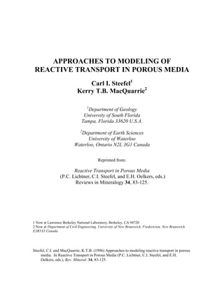
  • 25. Steefel MacQuarrie: Approaches to Modeling Reactive Transport which is referred to as the truncation error. It is possible to get a higher order (i.e. more accurate) approximation of the derivative ∂C/∂x by using a central difference approximation. If we use a Taylor expansion of the concentration written with respect to the points xi and xi−1 Ci−1 = Ci − ∂C ∂x xi xi − xi−1 1! + ∂2C ∂x2 xi (xi − xi−1)2 2! − . . . (83) and subtract this equation from Equation (80), we find that the truncation error is given by ∂C ∂x − Ci+1 − Ci−1 2xi = − (xi)2 6 ∂3C ∂x3 xi − . . . (84) In this expression, the second derivative terms have canceled so that only terms of the order (x)2 are neglected. The lowest order term which is neglected is said to be the order of the approximation. The central difference approximation of the first derivative is therefore said to be a second-order approximation while the forward difference scheme is a first-order approximation. As is readily apparent from the Taylor series expansion, the central difference approximation is second-order only when the grid spacing is constant (otherwise the second derivative terms do not completely cancel). Based on this criteria alone, the central difference approximation would be preferred because it includes less error than the first-order forward difference approximation. Higher order approximations are also possible. This kind of simple analysis of the error in various finite difference approximations would suggest that it is always preferable to use the higher order approximation since it is more accurate. Things are not quite so simple, however, since as we shall see below, the higher order approximations may introduce spurious oscillations (i.e. they may not be monotone). This is particularly true in the case of high Peclet number transport. Grid Peclet number. The Peclet number is a non-dimensional term which compares the characteristic time for dispersion and diffusion given a length scale with the characteristic time for advection. In numerical analysis, one normally refers to a grid Peclet number Pegrid = vx D (85) where v = q/θw is the average linear (pore water) velocity and the characteristic length scale is given by the grid spacing x. The problem with the central difference approximation for the first derivative term appears at grid Peclet numbers 2 (Unger et al., 1996). At grid Peclet numbers below 2 (i.e. dispersion/diffusion and advection are either of approximately the same importance or the system is dominated by dispersion and/or diffusion), the central difference approximation is monotone. Figure 2 shows a numerically calculated concentra- tion profile using a central difference approximation for the first derivative at a grid Peclet number of 20. Note that while the central difference scheme captures the overall topology and position of the front (reflecting its higher order), it introduces spurious oscillations in the vicinity of the front. This problem, which is a feature of all the unmodified higher order schemes, becomes more severe as the grid Peclet number is increased. While in certain cases it may be possible to simply refine the grid (i.e. reduce x) so that the grid Peclet number is less than 2, this often leads to an intractable problem because of the excessive number of grid points needed. In contrast to the second-order accurate central difference approximation, the first order scheme representation of the first derivative can be made monotone if an upwind or upstream 23
  • 26. Steefel MacQuarrie: Approaches to Modeling Reactive Transport Figure 2: Oscillations occur in the vicinity of a concentration front using the central difference approximation at grid Peclet numbers greater than 2. This simulation uses a grid Peclet number of 20. scheme (also referred to as a donor cell scheme) is used. This consists of finite differencing the first derivative using the grid cell upstream (i.e. the cell from which the advective flux is derived) and the grid cell itself ∂C ∂x ≈ Ci − Ci−1 xi − xi−1 (86) where the i − 1 node is assumed to be upstream. The price for this monotone scheme, however, is that it introduces numerical dispersion because of the truncation of the terms greater than first-order (of order x). The result is shown for grid Peclet numbers of 1, 10, and 100 in Figure 3, comparing the analytical solution in each case with the numerical. Courant number. Another important non-dimensional parameter in numerical anal- ysis is the Courant or Courant-Friedrichs-Lewy (CFL) number. This parameter gives the fractional distance relative to the grid spacing traveled due to advection in a single time step CFL = vt x . (87) It is possible to show using a Fourier error analysis that for a forward difference in time ap- proximation (i.e. explicit), no matter what approximation is used for the spatial derivatives, that the transport equation is stable for values of the CFL 1. This stability constraint for explicit transport equations states that one cannot advect the concentration more than one grid cell in a single time step. Unger et al. (1996) derive the monotonicity constraints for a variety of spatial and temporal weighting schemes, and show that only fully-implicit trans- port methods are not subject to the CFL constraint. A similar expression may be derived for systems characterized by purely diffusive transport, giving rise to a diffusion number ND = D(t) (x)2 (88) where again the stability constraint for an explicit formulation is that ND be 1. Amplitude and phase errors. A Fourier analysis of the advection-dispersion equation can be carried out to show that there are different kinds of error associated with the upwind and the central difference approximations of the first derivative (Celia and Gray, 1992). One class of errors are amplitude errors which result in excessive smearing of a concentration 24
  • 27. Steefel MacQuarrie: Approaches to Modeling Reactive Transport Grid Peclet = 1 Grid Peclet = 10 Grid Peclet = 100 Concentration (uM) Distance (m) Concentration (uM) Concentration (uM) Figure 3: Effect of grid Peclet number on calculated concentration profiles using upwind, fully implicit formulation. front. The upwind formulation is characterized by significant amplitude errors except at a CFL number of 1 and using a forward in time discretization. In this case, the upwind scheme duplicates the analytical solution to within the resolution of the grid. The central difference approximation, in contrast, shows no amplitude errors throughout the range of CFL numbers. The central difference approximation of the first derivative, however, shows phase errors which result in the non-physical oscillation in the vicinity of a sharp front observed in Figure 2. The problems associated with the various schemes when applied to high Peclet number transport, therefore, are derived from more than one kind of error. Ideally, one would like to find a higher order scheme which is accurate because of its avoidance of amplitude errors while avoiding the phase errors associated with these methods (i.e. they are monotone). Finite element methods for spatial discretization Finite element techniques are very popular for solving transport problems, including transport in porous media. In one dimension, finite difference and linear finite element so- lutions obtained with the same nodal spacing have the same accuracy. The above discussion related to oscillations and numerical dispersion apply equally to finite element techniques, that is, grid Peclet and CFL criteria must be satisfied in order to obtain accurate and monotone solutions. There are, however, some important differences between standard finite differ- 25
  • 28. Steefel MacQuarrie: Approaches to Modeling Reactive Transport ence and finite element methods in two or three dimensional problems. Thus we present a very brief introduction to the concepts which form the basis for the finite element method. Complete treatment of the subject can be found in the literature, for example, Huyakorn and Pinder (1983) and Istok (1989) present detailed coverage for subsurface applications. The finite element method arrives at a solution in three steps. First, the domain is discretized and a trial solution consisting of an interpolation function (usually linear), which passes through the unknown nodal values of concentration, is constructed over the entire grid. Then, by demanding that the trial solution minimize the residual error, on average, a system of ODEs is obtained (one for each node in the grid). Finally, this system is converted into a set of algebraic equations by applying finite differences to the temporal derivative. If we consider a one-dimensional domain shown in Figure 4, we can approximate the concentration profile, C(x), in any element using linear interpolation functions Ĉ(x) = C1 1 − x Le + C2 x Le (89) where Ĉ(x) is the trial solution, C1 an C2 are the concentrations at node 1 and 2, respectively, and Le is the element length. This can also be written as Ĉ(x) = 2 j=1 Cj Nj (x) (90) where j is the nodal index for the element and Nj (x) are the basis functions for the linear element, that is N1(x) = 1 − x Le , N2(x) = x Le . (91) The method of weighted residuals (Huyakorn and Pinder, 1983) is usually used to minimize residual errors; often the weighting functions are chosen to be the same as the basis functions, which yields the Galerkin method. As an example, we present the integral equation for a steady-state diffusion problem R ∂ ∂x D ∂Ĉ(x) ∂x Nj (x)dx = 0 (92) where R is the domain region, and j=1 to NN, where NN is the total number of nodes in the domain. The trial solution, Equation (90), is next substituted into Equation (92) and the spatial derivative is reduced using integration by parts (Huyakorn and Pinder, 1983). The finite element method has the well known advantage that it can be applied with a variety of element shapes (in two and three dimensions) and is thus well suited for non- rectangular geometries. In two-dimensions, triangular elements with linear basis functions can be used to discretize almost any conceivable domain. Arbitrary discretization of a do- main, however, can lead to nonphysical results, for example mass diffusion from a node with a low concentration to a node with a higher concentration, and specific discretization criteria must be satisified (e.g. Cordes and Kinzelbach, 1996). An additional difference between finite element discretizations and standard finite difference methods in two or more dimen- sions is the ability of finite elements to easily handle off-diagonal terms in the disperson tensor. For example, if we apply finite differences in two dimensions, concentration gradi- ents are calculated along a line perpendicular to a surface (the interface between the nodes) 26
  • 29. Steefel MacQuarrie: Approaches to Modeling Reactive Transport C(x) node C(x) L x 1 2 3 C e Figure 4: Schematic of the trial solution to a continuous function. The linear interpolation functions commonly used in the finite element method are indicated when in fact tensor quantities present non-zero tangential components at this interface. Fer- raresi and Marinelli (1996) have suggested a correction to the integrated finite difference method to allow for transport deriving from tensor quantities; the proposed method borrows from the finite element concept of two-dimensional interpolation on discrete elements. It should be noted that control volume discretization can be applied using nonrectan- gular elements, and thus these more physically-intuitive methods can also be employed to discretize complex geometries (e.g. Forsyth, 1991; Di Giammarco et al., 1996). High-resolution spatial schemes. BecauseofthegreatinterestinnumericallysimulatinghighPecletnumbertransportsys- tems (the problem is not restricted to porous medium, but appears in all dynamical systems involving advection, including oceanography, atmospheric science etc.), a large number of alternative schemes have been proposed. These include the method of characteristics (or its modified versions) (e.g. Konikow and Bredehoeft, 1978; Arbogast et al., 1992; Chilakapati, 1993; Zheng and Bennett, 1995) and adjoint Eulerian-Lagrangian methods (Celia et al., 1990). Both of these approaches are based on the treatment of the advective part of the transport equation using a Lagrangian scheme (a reference frame in which one follows the advective displacement of the fluid packet). An Eulerian (fixed) reference frame is then used to simulate dispersive/diffusive transport. The approach reduces numerical dispersion by decreasing the effective grid Peclet number for the fixed Eulerian grid. These schemes can be used with finite element approaches as well. While somewhat more complicated than the simple approaches outlined above, they are capable in many systems of virtually eliminating numerical dispersion. For example, in the modified method of characteristics as developed by Chilakapati (1993), one computes the changes in concentration at a grid point by tracking back along a fluid streamline to the starting point of a fluid packet at the beginning of a time step. This elegant approach, however, can be difficult to implement in physically heterogeneous two- and three-dimensional systems where the streamline map- ping can become very complicated. In addition, to obtain good results it may be necessary to track a large number of fluid packets, thus quickly leading to excessive CPU time and memory requirements. Nonetheless, the method of characteristics and related approaches are still widely used when it is critical that numerical dispersion be avoided. 27
  • 30. Steefel MacQuarrie: Approaches to Modeling Reactive Transport Another class of high resolution Eulerian methods uses higher-order approximations for the first derivatives, but hybridizes these with low-order schemes in an attempt to obtain monotone solutions. The solutions have the higher-order accuracy in smooth regions and the low-order accuracy near discontinuities (e.g. near plume fronts). The price to be paid for these schemes is that they are nonlinear, even when applied to initially linear problems such as Equation (79). In this class are the flux-corrected transport (FCT) methods (Boris and Book, 1973; Oran and Boris, 1987; Zalesak, 1987; Hills et al., 1994) which normally give excellent results when applied to non-reactive solute transport (Hills et al., 1994; Yabusaki et al., in prep.). However, as in some of the other methods discussed here, very low level oscillations still exist which can give spurious results when nonlinear reactions are coupled into the solution. In an example given below we solve for reactive transport in a physically heterogeneous domain using a 4th order FCT scheme. We have found that another scheme, referred to as the total variation diminishing or TVD scheme, gives more nearly oscillation-free behavior (Harten, 1983; Sweby, 1984;Yee, 1987; Gupta et al., 1991). The TVD method is one of a class of methods which use limiters to ensure monotonicity of the solution (Van Leer, 1977a,b; Leonard, 1979a,b; Leonard, 1984). In the example below, we use the implementation of the TVD suggested by Gupta et al. (1991) which is combined with a third-order Leonard scheme (Leonard, 1979b). Example of reactive transport in a physically heterogeneous porous media. Although a thorough review of the high resolution monotone methods is beyond the scope of this work, it is useful to compare two of the schemes with which we have extensive experience. As an example problem, consider the influx of a groundwater containing initially 0.1 M dissolved organic carbon (DOC) through the left boundary of a physically heterogeneous domain. Organic carbon degrades by a first-order rate law via sulfate reduction according to the reaction CH2O + 1 2 SO2− 4 −→ HCO− 3 + 1 2 HS− + 1 2 H+ . (93) SO2− 4 is replenished in solution by the equilibrium dissolution of gypsum (CaSO2− 4 ·2H2O) while the carbonate produced is largely consumed by the equilibrium precipitation of calcite (CaCO3). Flow is from left to right across the domain. Downstream of the front, the groundwater is in equilibrium with calcite and gypsum and should be unaffected by the front upstream. Since the medium is assumed to be chemically homogeneous, the initial aqueous concentrations computed from the equilibrium relations are homogeneous as well. The simulation was run as a pure advective problem using the FCT (Hills et al., 1994) and TVD (Gupta et al., 1991) algorithms and using a 200 by 88 grid. The calculation was carried out with MCTRACKER, a massively parallel version of the code OS3D (Steefel and Yabusaki, 1996). The simulations were run on a CM-5 massively parallel computer using 32 to 128 processors. The T OT Ca+2 concentration is shown after 0.5 days in Figure 5. The TVD method shows increased Ca+2 concentrations about 1/3 of the way across the domain, with the leading edge of the concentration front matching the position of a tracer released at the same time as the organic carbon plume. Downstream of the front, essentially nothing is happening in the TVD simulation, which is the expected behavior. In contrast, the FCT method shows low-level oscillations both within the organic carbon plume and downstream of the front. It should be noted that these oscillations are not evident when the tracer concentration is plotted at the same time; the low-level oscillations (or non-monotonicity) characteristic of the 4th order FCT become amplified when nonlinear chemistry is involved. We have also carried out other calculations on an equilibrium redox problem using the 4th order FCT where the method failed due to the low-level oscillations interacting with the highly nonlinear chemistry (Regnier et al., in press). A transport scheme based on the well- known Lax-Wendroff scheme (Press et al., 1986) also failed on this problem. In contrast, 28
  • 31. Steefel MacQuarrie: Approaches to Modeling Reactive Transport 100 200 0 0 25 50 75 0 25 50 75 Distance (cm) 15 16 17 18 FCT TVD Distance (cm) mM Figure 5: Comparison of the 4th order FCT method (Hills et al., 1994) and the 3rd order TVD method (Gupta et al., 1991) on a problem involving organic carbon degradation via sulfate reduction coupled to two equilibrium dissolution-precipitation reactions. The non-monotone character of the FCT algorithm, although not detectable in a plot of non-reactive solute concentrations, results in unacceptable oscillations when amplified by nonlinear chemical reactions. In contrast, the TVD method performs much better on this reactive transport problem. the problem was solved with both upwind and 3rd order TVD formulations. This points out that care must be taken in evaluating transport algorithms. Many, like the well-known Lax-Wendroff scheme and the FCT scheme evaluated here, are not sufficiently monotone that they can be used on the highly nonlinear reactive transport problems that often occur in hydrogeology. METHODS FOR COUPLING REACTION AND TRANSPORT In recent years much of the discussion about numerical approaches to reactive transport has centered on the question of how to couple the reaction and transport terms. The reaction term affects the local concentrations which in turn determine the fluxes of aqueous species. In the same way, the magnitude of the fluxes can affect the reaction rates. An accurate solution of the overall problem, therefore, requires that the terms be coupled at some level. Several methods have been proposed to solve the coupled set of equations. The most straightforward way conceptually, but the most demanding from a computational efficiency pointofview, istosolvethegoverningequations, includingbothreactionandtransportterms, simultaneously. This approach is referred to as a one-step or global implicit method (Kee et al., 1987; Oran and Boris, 1987; Steefel and Lasaga, 1994; Steefel and Yabusaki, 1996). Alternatively, it is possible to use operator splitting techniques to decouple the reaction and transport calculations. The classic time-splitting approach to solving the coupled set of equations (referred to by T. Xu [pers. comm., 1996] as the sequential non-iterative approach 29
  • 32. Steefel MacQuarrie: Approaches to Modeling Reactive Transport or SNIA) consists of solving the reaction and transport equations within a single timestep in sequence, with no iteration between the two. A method championed byYeh and Tripathi (1989; 1991) is the sequential iteration approach or SIA where the reaction and transport are solved separately but iteration between the two calculations is carried out until a converged solution is attained. There are variants on these approaches, including a predictor-corrector approach (Raffensperger and Garven, 1995) and the Strang splitting approach (Zysset and Stauffer, 1992). The formulations are discussed below and their performance is compared on several test problems. One-step or global implicit approach Since the publication of the influential paper byYeh and Tripathi (1989) which rejected the use of the one-step or global implicit approach as being too CPU time and memory intensive, relatively little discussion of one-step approaches for the reaction-transport prob- lem has appeared in the hydrogeochemical literature. This is despite the fact that the global implicit approach has been used sucessfully for some time in the chemical and mechanical engineering fields (Kee et al., 1987), although even in these fields the relative merits of the decoupled or operator splitting approaches versus the one-step approach still rages (Oran and Boris, 1987; Kee et al., 1987). In one component systems (for example, modeling of the system quartz-SiO2(aq) or stable isotope exchange) or in systems in which there is no coupling via reactions of the various species and minerals, there is no particular difficulty in simply solving the entire system using standard iterative or direct linear algebra methods. In this case, the presence of a reaction term does not increase the size of the matrix over and above its size in the case of transport alone. Using as an example a one-dimensional diffusion-reaction problem where the porosity, diffusion coefficient, and grid spacing are assumed constant, the fully implicit approach in finite difference form is given by Cn+1 − Cn t = D Cn+1 i+1 − 2Cn+1 i + Cn+1 i−1 X2 + R(Cn+1 i ) (94) where i, i − 1, and i + 1 refer to the location of the nodal points and n and n + 1 refer to the present and future time levels respectively. Note that the form of Equation (94) assumes that the values of the concentration which appear in the accumulation term (the left hand side), the transport term, and the reaction term are those at the future time level. If the reaction term R is linear, Equation (94) can be rewritten as a set of simultaneous linear equations of the form b1C1 + c1C1 = d1 (95) a2C1 + b2C2 + c2C3 = d2 (96) · · · (97) aN−1CN−2 + bN−1CN−1 + cN−1CN = dN−1 (98) aN CN−1 + bN CN = dN (99) where the lower case characters ai, bi, and ci are the coefficients, di refers to the right hand side, and N is the number of spatial points. The one-dimensional system can be represented by a tridiagonal matrix of the form      b1 c1 0 · · · a2 b2 c2 · · · · · · · · · aN−1 bN−1 cN−1 · · · 0 aN bN           C1 C2 · · · CN−1 CN      =      d1 d2 · · · dN−1 dN      (100) 30
  • 33. Steefel MacQuarrie: Approaches to Modeling Reactive Transport which is easily and rapidly solved with the Thomas algorithm (Press et al., 1986). The reaction term, if present, is imbedded in the coefficient bi multiplying the concentration at the nodal point i. Since the transport equations are linear themselves, no iteration is required unless the reaction terms are nonlinear. The problem is only slightly more difficult in the case of two and three dimensional transport. In two dimensions where a 5 point stencil is used (Fig. 1), any one row of the coefficient matrix will have 5 non-zero entries. Since the system is still sparse, however, it can be readily solved in most cases using modern sparse matrix solvers (e.g. WATSOLV, VanderKwaak et al., 1995). Again, where there is no coupling between species introduced by the reactions, each species concentration field can be solved for independently of the other species in the system. Using a global implicit approach becomes considerably more difficult in the case of a multicomponent, multi-species system both because the coupling of species via reactions enlarges the size of the coefficient matrix and because it typically results in sets of nonlinear equations which must be solved. Just as in the case of the time-dependent reaction systems, the nonlinearities resulting from the reaction terms require the use of iterative methods. The Newton-Raphson technique described above can be used, however, to solve the global set of equations, i.e. a set of equations containing both transport and reaction terms (Steefel and Lasaga, 1994). The size of the Jacobian matrix which must be constructed and solved becomes considerably larger since each function will include contributions from the con- centrations both at that nodal point itself and from neighboring nodal points which are used in the finite difference or finite element discretization. For example, in the case of one- dimensional transport and Nc unknown concentrations at each nodal point, the form of the Newton equations to be solved is Nc k=1 ∂fi,j ∂Ck,j δCk,j + Nc k=1 ∂fi,j ∂Ck,j+1 δCk,j+1 + Nc k=1 ∂fi,j ∂Ck,j−1 δCk,j−1 = −fi,j (101) where i refers to the component number, k is the unknown component species number, and j, j +1, and j −1 are the nodal points. The Jacobian matrix in the case of one-dimensional transport takes a block tridiagonal form      A1,1 A1,2 0 · · · A2,1 A2,2 A2,3 · · · · · · · · · AN−1,N−2 AN−1,N−1 AN−1,N · · · 0 AN,N−1 AN,N           δC1 δC2 · · · δCN−1 δCN      = −      f1 f2 · · · fN−1 fN      (102) where the entries in the Jacobian matrix (the A) are submatrices of dimension Nc by Nc in the case where there are Nc unknowns. The entries δCi refer here to the entire vector of unknown concentrations at any particular nodal point while the functions fi include the entire vector of equations for the unknown concentrations at each nodal point. The one-dimensional problem can be solved relatively rapidly using a block tridiagonal solver (Steefel and Lichtner, 1994; Hindmarsh, 1977). In the case of multidimensional systems, the equations can be solved by block iterative methods (Steefel and Lasaga, 1994) or by using sparse matrix solvers which in certain cases require minor modifications to handle the block structure of multicomponent problems (VanderKwaak et al., 1995; Steefel and Yabusaki, 1996). The major obstacle to the use of global implicit methods for multicomponent reactive transport systems is the need for large amounts of computer memory (Yeh and Tripathi, 31