1. Computer Exercise (RStudio)
> data_ksubs<-read.csv("data_ksubs (1).csv")
> View(data_ksubs)
1.
a)
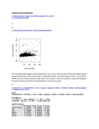
> plot(data_ksubs$inc, data_ksubs$nettfa)
The resulting model suggests heteroskedasticity; one can see, when we plot net financial wealth against
annual family income, the concentration on data points within a specific range of income. As we move
further out, the variation becomes wider and is not constant. One can see points scattered throughout
the graph and because of this, homoscedasticity cannot be assumed.
b)
> ols.fit <- lm(nettfa ~ inc + age + agesq + male + e401k, data = data_ksubs)
> summary(ols.fit)
Call:
lm(formula = nettfa ~ inc + age + agesq + male + e401k, data = data_ksubs)
Residuals:
Min 1Q Median 3Q Max
-508.60 -18.71 -3.38 9.95 1462.18
Coefficients:
Estimate Std. Error t value
(Intercept) 5.22945 10.11065 0.517
inc 0.94712 0.02634 35.954
age -2.38888 0.49058 -4.869
agesq 0.03975 0.00563 7.061
male 4.22406 1.50898 2.799
e401k 6.73346 1.28603 5.236

2. Pr(>|t|)
(Intercept) 0.60501
inc < 2e-16 ***
age 1.14e-06 ***
agesq 1.78e-12 ***
male 0.00513 **
e401k 1.68e-07 ***
---
Signif. codes:
0 ‘***’ 0.001 ‘**’ 0.01 ‘*’ 0.05 ‘.’ 0.1 ‘ ’ 1
Residual standard error: 58.07 on 9269 degrees of freedom
Multiple R-squared: 0.1762, Adjusted R-squared: 0.1757
F-statistic: 396.5 on 5 and 9269 DF, p-value: < 2.2e-16
c)
> N <-dim(data_ksubs)[1]
> part.out.fit <- lm(inc ~ age + agesq + male + e401k, data = data_ksubs)
> std.beta1 <- sqrt((N/(N-5))*sum((residuals(part.out.fit)^2)*(residuals(ols.
fit)^2))/(sum(residuals
+
(part.out.fit)^2))^2)
Heteroskedasticity robust standard error for annual family income; compared with standard error in the
estimation in b)
> std.beta1
[1] 0.07513404
> coef(summary(ols.fit))[2,2]
[1] 0.02634275
> std.beta1/coef(summary(ols.fit))[2,2]
[1] 2.852172
> part.out.fit <- lm(age ~ inc + agesq + male + e401k, data = data_ksubs)
> std.beta2 <- sqrt((N/(N-5))*sum((residuals(part.out.fit)^2)*(residuals(ols.
fit)^2))/(sum(residuals
+
(part.out.fit)^2))^2)
Heteroskedasticity robust standard error for age; compared with standard error in the estimation in b)
> std.beta2
[1] 0.5996238
> coef(summary(ols.fit))[3,2]
[1] 0.4905835
> std.beta2/coef(summary(ols.fit))[3,2]
[1] 1.222267
> part.out.fit <- lm(agesq ~ inc + age + male + e401k, data = data_ksubs)
> std.beta3 <- sqrt((N/(N-5))*sum((residuals(part.out.fit)^2)*(residuals(ols.
fit)^2))/(sum(residuals
+
(part.out.fit)^2))^2)
Heteroskedasticity robust standard error for agesq; compared with standard error in the estimation in b
)

3. > std.beta3
[1] 0.007472046
> coef(summary(ols.fit))[4,2]
[1] 0.005629612
> std.beta3/coef(summary(ols.fit))[4,2]
[1] 1.327275
> part.out.fit <- lm(male ~ inc + age + agesq + e401k, data = data_ksubs)
> std.beta4 <- sqrt((N/(N-5))*sum((residuals(part.out.fit)^2)*(residuals(ols.
fit)^2))/(sum(residuals
+
(part.out.fit)^2))^2)
Heteroskedasticity robust standard error for male; compared with standard error in the estimation in b)
> std.beta4
[1] 1.447424
> coef(summary(ols.fit))[5,2]
[1] 1.50898
> std.beta4/coef(summary(ols.fit))[5,2]
[1] 0.9592073
> part.out.fit <- lm(e401k ~ inc + age + agesq + male, data = data_ksubs)
> std.beta5 <- sqrt((N/(N-5))*sum((residuals(part.out.fit)^2)*(residuals(ols.
fit)^2))/(sum(residuals
+
(part.out.fit)^2))^2
Heteroskedasticity robust standard error for e401k; compared with standard error in the estimation in b
)
> std.beta5
[1] 1.494642
> coef(summary(ols.fit))[6,2]
[1] 1.286028
> std.beta5/coef(summary(ols.fit))[6,2]
[1] 1.162216
d)
> ci.homo <- ols.fit$coefficients[2] + c(-qnorm(0.975),qnorm(0.975))*coef(su
mmary(ols.fit))[2,2]
> ci.heter <- ols.fit$coefficients[2] + c(-qnorm(0.975),qnorm(0.975))*std.bet
a1
> ci.homo
[1] 0.8954945 0.9987561
> ci.heter
[1] 0.7998653 1.0943853
Interpretation: When we compare the confidence interval for β1 using the homoscedastic standard error
with the confidence interval using the heteroskedastic robust standard error, we see that the c.i. for the
heteroskedastic robust standard error is wider.
Additional Information:
Test for heteroskedasticity (Breush-Pagan)

4. > test.lin <- lm(I(residuals(ols.fit)^2) ~ inc + age + agesq + male + e401k,d
ata=data_ksubs)
> summary(test.lin)
Call:
lm(formula = I(residuals(ols.fit)^2) ~ inc + age + agesq + male +
e401k, data = data_ksubs)
Residuals:
Min 1Q Median 3Q Max
-43169 -5271 -1235 2159 2121900
Coefficients:
Estimate Std. Error t value
(Intercept) 7251.699 8151.187 0.890
inc 280.903 21.237 13.227
age -895.444 395.507 -2.264
agesq 12.383 4.539 2.728
male 1310.332 1216.537 1.077
e401k -1534.153 1036.793 -1.480
Pr(>|t|)
(Intercept) 0.37368
inc < 2e-16 ***
age 0.02359 *
agesq 0.00638 **
male 0.28146
e401k 0.13898
---
Signif. codes:
0 ‘***’ 0.001 ‘**’ 0.01 ‘*’ 0.05 ‘.’ 0.1 ‘ ’ 1
Residual standard error: 46820 on 9269 degrees of freedom
Multiple R-squared: 0.02158, Adjusted R-squared: 0.02105
F-statistic: 40.88 on 5 and 9269 DF, p-value: < 2.2e-16