MAE598 Applied CFD Project#1 Water Tank Analysis

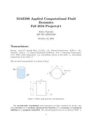
MAE598 Applied Computational Fluid
Dynamics
Fall 2016 Project#1
Aditya Vipradas
ASU ID: 1209435588
October 12, 2016
Nomenclature
Density: ρ(kg/m3
), Specific Heat: Cp(J/kg − K), Thermal Conductivity: K(W/m − K),
Viscosity: µ(kg/m − s), Thermal Expansion Coefficient: β(K−1
), Operating Temperature:
t(o
C), Water outlet temperature: Tout, non-uniform velocity at the outlet: νn, non-uniform
temperature at the outlet: T.
The hot water tank geometry is as shown in Fig.1.
Figure 1: Water tank geometry and dimensions
The second-order tetrahedral mesh parameters are kept consistent for all the cases
with relevance set to medium, advanced size function set to curvature and advanced
inflation set to program controlled. The material properties are set as shown in Table. 1.
1

Material Properties
• ρ : 2719
Water container (aluminum) • Cp : 871
• K : 202.4
• ρ : 989.7576
• Cp : 4216
Water • K : 0.677
• µ : 8e−4
• β : 4.2827e−4
Table 1: Material Properties
The density of water is not constant. It is considered to vary with the water temperature
according to the Boussinesq approximation. This allows natural thermal convection due to
buoyancy. The Boussinesq approximation only updates the density terms associated with
gravitational acceleration g. Thus, gravity is set ”on” in ANSYS Fluent. It is expected that
hot water should rise and cold water should settle on the container base plate. The water
density and thermal expansion coeﬃcient in Table. 1 is calculated at an operating temperature
of 318K (45o
C) using the Kell’s formulation in Eq. 1 and 2 respectively. These equations are
calculated at an operating pressure of 101.325 kPa.
ρ =
999.84 + 16.95t − 7.99 ∗ 10−3
t2
− 46.17 ∗ 10−6
t3
+ 105.56 ∗ 10−9
t4
− 280.54 ∗ 10−12
t5
1 + 16.9 ∗ 10−3t
(1)
β =
−1
ρ
dρ
dt
(2)
The material properties are set as shown in Figs.2 and 3. The Boussinesq approximation is
set by clicking: (Deﬁne – Operating Conditions).
Figure 2: Water material properties using Boussinesq implementation
2

Figure 3: Aluminum material properties
The boundary conditions are set as shown in Figs.4, 5 and 6. The tank base is externally
maintained at 65o
C or 338K. The container base plate roughness height is set to a standard
value of 1e − 6m.
Figure 4: Water inlet boundary conditions
Figure 5: Water outlet boundary conditions
3

Figure 6: Tank base boundary conditions
The water outlet temperature is calculated as the average of temperature weighted by
flow rate as in Eq.3. This is performed in each case as shown in Fig.7. Set the expressions
by clicking: (Define – Custom Field Functions) and integrate over the area by clicking:
(Reports – Surface Integrals).
Tout =
νnTdA
νndA
(3)
(a) Defining numerator in custom field function (b) Defining denominator in custom field
function
(c) Integrating numerator over water outlet area (d) Integrating denominator over water outlet
area
Figure 7: Calculating Tout using Eq. 3
4

The convergence residuals are set as shown in Table. 2.
Residual Absolute Criteria
continuity 0.001
x-velocity 0.001
y-velocity 0.001
z-velocity 0.001
energy 1e-06
k 0.001
epsilon 0.001
Table 2: Residual Criteria
Solution convergence is checked through the original residual plots and adapted mesh
residual plots. Temperature gradient based mesh adaptation can be performed in each case
as shown in Fig.8. The Reﬁne Threshold is set at 10% of the maximum temperature gradient.
Procedure: (Adapt – Gradient).
Figure 8: Mesh adapt based on temperature gradient
Solution convergence is ensured by checking mass and energy balance of the system along
with the convergence in residual plots. Mass (M) and energy (H) equations are given in Eq.
4 and 5 respectively.
M = νnρdA (4)
H = νnρCpTdA (5)
5

The Fluxes and Custom Field Functions options are used to ensure the mass and
energy balance respectively as shown in Figs. 9 and 10.
Figure 9: Mass balance evaluation
Figure 10: Energy balance evaluation
6

1 Task 1: Case A
In Case A: H = 1m, D = 0.5m, d = 0.04m, L = 0.1m, Z1 = 0.8m, Z2 = 0.2m. The
hot water tank is symmetrically model about ZX plane as shown in Fig. 11 to reduce the
computation cost .
(a) CAD model (b) Tetrahedral mesh
(c) CAD model (d) Tetrahedral mesh
Figure 11: Water tank model in ANSYS Workbench
The material properties and boundary conditions are set as explained previously. 858 cells
are marked for adaptation and the total number of cells increases from 40672 to 46678. The
solution converges with the scaled residuals chart as shown in Fig.12.
7

(a) Original scaled residuals after 472 iterations
(converges)
(b) Adapted scaled residuals after 516 iterations
(converges)
Figure 12: Solution convergence
Mass (kg/s) and energy (J/s) for this case are conserved as seen in Table. 3.
Water Inlet Water Outlet
Mass 0.0306 -0.0307
Energy 38425.91 40902.87
Table 3: Mass and energy balance
The Tout for Task1: Case A is calculated using Eq.3 and equals 311.0125 K.
The deliverables for this task are as follows:
Figure 13: Temperature contour plot on symmetry plane
8

(a) Temperature contour plot on the c/s at Z =
0.2 m
(b) Temperature contour plot on the c/s at Z =
0.8 m
Figure 14: Temperature contour plots
(a) Streamline on the symmetry plane (b) Streamline in the container
Figure 15: Streamline plots
2 Task 1: Case B
In Case B: H = 1m, D = 0.5m, d = 0.04m, L = 0.1m, Z1 = 0.2m, Z2 = 0.8m. The
hot water tank is symmetrically modeled about ZX plane as shown in Fig. 16 to reduce the
computation cost .
9

(c) CAD model (d) Tetrahedral mesh
The material properties and boundary conditions are set as explained previously. 1705
cells are marked for adaptation and the total number of cells increases from 52418 to 64353.
The solution converges with the scaled residuals chart as shown in Fig.17.
(converges)
(b) Adapted scaled residuals after 1093
iterations (converges)
10

Mass 0.0306 -0.0306
Energy 38425.97 40442.35
The Tout for Task1: Case B is calculated to be 310.0846 K.
0.2 m
0.8 m
11

Thus, for Task 1,
Case A Case B
Temperature (K) 311. 0125 310.0846
Table 5: Water outlet temperatures (K)
As seen in Table. 5, the Tout in Case A is greater than that in Case B . Even though the
difference is not that significant, some rationales can be drawn to explain this difference.
1. As observed from the streamline plots of both the cases, water from the inlet in Case A
is in contact with the heating base over a larger area (almost complete) as compared to
that in Case B. In Case B, the inlet water does not come in contact with a portion of
heating base area near the inlet as seen in Fig.20. The hot base is the primary source
of temperature increase in water through conduction.
2. In Case A, as seen from Figs.15 and 13, water vortex as seen in the streamline plots
is formed in the region where the temperature is considerably higher (more than 310
K) whereas Figs.20 and 18 show that the water vortex forms in the region where the
temperature is relatively lower (about 308 K). This results into more heat transfer in
Case A due to buoyant natural convection.
3. Water in Case A falls from a greater height than that in Case B. Thus, it has more
energy as compared to Case B which eventually results in a larger heat dissipation and
temperature increase as it strikes the container base. This is a minor detail but it
contributes to the small temperature difference in both the cases.
4. Also, heat transfer at the base in Case B should be more due to larger temperature
gradient. This is because the water inlet in Case B is closer to the base as compared to
Case A. But the three reasons mentioned above seem predominant resulting in a larger
water outlet temperature in Case A.
12

3 Task 2: Case C
In Case C: H = 1m, D1 = 0.625m, D2 = 0.4m, d = 0.04m, L = 0.1m, Z1 = 0.2m, Z2 = 0.8m.
Total volume of main tank remains the same as that of the design in Task 1 as shown in Fig.
21. The hot water tank is symmetrically modeled about ZX plane as shown in Fig. 22 to
reduce the computation cost.
Figure 21: Elliptical cross section of the water tank
13

(converges)
(converges)
Mass 0.0306 -0.02930
Energy 38425.99 40308.45
The Tout for Task2: Case C is calculated to be 311.3155 K.
14

0.2 m
0.8 m
The given container being a heat pump, the efficiencies of elliptical and circular designs
are measured in terms of their coefficients of performance as given in Eq.6.
COP =
TH
TH − TC
(6)
Here, TH and TC are water outlet and inlet temperatures respectively. The COPs obtained
are as shown in Table. 7. Here, given that the cross-sectional areas are the same in cases
Case B (circular) Case C (elliptical)
COP 25.67 23.38
Table 7: Coefficients of Performance
B and C, for the given mesh, the heat flux from the base should be equal. But as seen in
the simulation, it is 1560 W for Case B and 1735 W for Case C. This is due to different
15

mesh at the container base. The work consumed i.e. water inlet height is same in both the
cases. Therefore, ideally, COP and water outlet temperatures for cases B and C should be
the same. Here, COPB is larger than COPC due to the diﬀerent heat ﬂux values. The outlet
temperature in Case C is larger as seen in Table. 8.
Case B (circular) Case C (elliptical)
Outlet Temperature (K) 310.0846 311.3155
Table 8: Outlet Temperatures
4 Task 2: Case D
In Case D: H = 1m, D1 = 0.4m, D2 = 0.625m, d = 0.04m, L = 0.1m, Z1 = 0.2m,
Z2 = 0.8m. Total volume of the main tank remains the same as the design in Task 1 as shown
in Fig. 21. The hot water tank is symmetrically modeled about ZX plane as shown in Fig.
27 to reduce the computation cost.
16

(converges)
(converges)
Mass 0.0306 -0.0307
Energy 38452.99 41951.39
The Tout for Task2: Case D is calculated to be 311.3222 K.
17

0.2 m
0.8 m
The COPs obtained for this case from Eq.6 are as shown in Table. 10. Here, given that
Case B (circular) Case D (elliptical)
COP 25.67 23.37
Table 10: Coefficients of Performance
the cross-sectional areas are the same in cases B and D, for the given mesh, the heat flux from
the base should be equal. But as seen in the simulation, it is 1560 W for Case B and 1730
W for Case D. This is due to different mesh at the container base. The work consumed i.e.
water inlet height is same in both the cases. Therefore, ideally, COP and outlet temperature
for cases B and D should be the same. Here, COPB is larger than COPD due to the different
heat flux values. The outlet temperature in Case D is larger as seen in Table. 11.
18

Case B (circular) Case D (elliptical)
5 Task 3
The geometry in this task is the same as that in Task 1: Case A.
The material properties and boundary conditions are set as explained previously except
that the water density is set constant and gravity eﬀects are turned ”oﬀ”. 836 cells are
marked for adaptation and the total number of cells increases from 40672 to 46524. The
(converges)
(converges)
Mass 0.0306 -0.0306
Energy 38425.91 38694.71
The Tout for Task3 is calculated to be 300.8424 K.
19

0.2 m
0.8 m
20

When the density is set constant and gravity is turned ”off”,
1. There is no buoyancy driven natural convection in the fluid due to the Boussinesq
approximation.
2. Thus, motion of hot and cold water is not driven due to density difference in them.
3. Heat transfer only takes place due to heat conduction from the bottom plate and thus
major portion of the fluid in the container is close to 298 K (temperature of cold water).
4. The water outlet temperature is significantly lower (300.84 K) as compared to that in
tasks 1 and 2.
5. Water flow is driven only by the inlet velocity and not by gravity.
6 Task 4
The geometry in this task is the same as that in Task 1: Case B.
The heat flow from the bottom plate into the tank is obtained by using the Total Heat
Transfer Rate option in the Fluxes menu as shown in Fig.36.
Figure 36: Heat transfer rate estimation
Thus, the total heat flow rate from the bottom plate into the tank is 1559.466 W.
To obtain the average heat flux, the total heat flow rate obtained is divided by half the
cross-sectional area of the bottom plate as shown in Eq.7.
HeatFluxavg =
1559.466
π
8
0.52
= 15884.59W/m2
(7)
The constant temperature condition on the bottom plate is replaced with that of the
constant heat flux (15884.59W/m2) as shown in Fig.37.
21

Figure 37: Applying constant heat ﬂux condition
The material properties and boundary conditions are set as explained previously. The
Figure 38: Scaled residuals (converges)
Mass 0.0306 -0.0306
Energy 38425.97 40476.43
The Tout for Task4 is calculated to be 310.0598 K.
This temperature is exactly equal to the outlet temperature obtained in Task 1: Case B
as seen in Table. 14.
22

Task 4 Task 1: Case B
The reason for this is that the constant temperature condition of 338K generates the heat
ﬂux of 15884.59W/m2
. Therefore, providing the constant temperature condition of 338K or
heat ﬂux condition of 15884.59W/m2
gives the same results and eventually the same water
outlet temperature.
Outlet Temperature Results
Case A Case B Case C Case D Task 3 Task 4
Outlet Temperature (K) 311.0125 310.0846 311.3155 311.3222 300.8424 310.0598
23

7 Challenge 1 [Aditya Vipradas (1209435588)]
Collaborated with Abhijeet Durgude (1209679741)
The geometry in this task is the same as that in Task 1: Case B. The temperature imposed
on the bottom plate is non-uniform time-independent as given in Eq. 8.
T(r) = 65exp(−r/D) (8)
This temperature is in o
C, r is the radial distance at the bottom plate. The non-uniform
temperature is imposed using a User-Defined Function (UDF) in Fluent. The UDF is programmed
in Notepad as shown in Fig. 39.
Figure 39: UDF for non-uniform temperature
As seen in the C Program, the F CENTROID function in udf.h outputs the centroids of
each cell of a given face f. These centroids are used to calculate the radial distance r which
is used to define the temperature profile in F PROFILE function. 273 is added to convert the
temperature in K. The .c programme file is interpreted in Fleunt (Procedure: Defined -
User-Defined - Functions - Interpreted). The boundary condition is applied by selecting
the respective programme file in the Temperature section of the bottom plate boundary
condition.
Figure 40: Impose the non-uniform temperature boundary condition
24

The temperature proﬁle obtained on the bottom plate is as shown in Fig.41.
Figure 41: Temperature proﬁle on the bottom plate
The Tout for Challenge 1 is calculated to be 304.8164 K.
25

0.2 m
0.8 m
Challenge 1 Task 1: Case B
As seen, the outlet temperature in challenge 1 is lower than that in Task 1: Case B as
expected.
26

No Collaboration
The geometry in this task is the same as that in Task 1: Case A. The dependence of
temperature on varying inlet velocity is evaluated in this task. The ParametricDesign tool is
used for this purpose. The inlet velocity input parameter is defined as shown in Fig. 45. The
numerator and denominator surface integrals over the outlet and mid-plane areas are defined
as the output parameters
Figure 45: Defining input and output parameters
As seen in this figure, the X-velocity in the inlet is defined as the input parameter, whereas,
the numerator and denominator surface integrals from Eq.3 over outlet and mid-plane areas
are defined as the output parameters. The Fluent box in ANSYS changes as shown in Fig.46.
Clicking the Parametric Set option and solving for all the design points yields the output
as shown in Fig.47.
Figure 46: Parametric Design
27

Figure 47: Parametric Design Output
As seen in Fig.47, P2: Numerator surface integral over outlet area, P3: Denominator
surface integral over outlet area, P4: Numerator surface integral over mid-plane area, P5:
Denominator surface integral over mid-plane area. Thus,
Tout =
P2
P3
(9)
Tmid =
P4
P5
(10)
The outlet and mid-plane temperatures are obtained by exporting the parametric data in
Excel as shown in Fig.48.
Figure 48: Tout and Tmid temperature calculations
The line plots for Tout and Tmid are as shown in the Figs. 49 and 50.
28

Figure 49: Tout vs Vin plot
Figure 50: Tmid vs Vin plot
As seen in Fig.49, the outlet temperature is lower for 0.01m/s inlet velocity because of
increase in the back-ﬂow due to low inlet velocity. The Tmid increases with decrease in Vin as
seen in Fig.50.
29

MAE598 Applied Computational Fluid
Dynamics
Fall 2016 Project#2
Aditya Vipradas
ASU ID: 1209435588
November 9, 2016
1 Common Simulation Procedure
Create the respective geometry in DesignModeler and mesh it according to the given
criteria in ANSYS Workbench. Use Pressure-Based solver and turn Gravity on. Select
the Multiphase model with 2 Volume of Fluids. Set Implicit Body Force on. Use the
required material properties from the Fluent Database. In Solution Methods, select the
Pressure-Velocity Coupling to PISO given the transient simulations with large time steps.
Use PRESTO! pressure spatial discretization scheme. Change the Pressure Under-Relaxation
Factor to 0.9.
The entire domain is occupied by Phase-1 by default. In order to add Phase-2 in it, adapt
the region using Adapt - Region - Mark by specifying the corresponding coordinates as
shown in Fig.1. Once, the region is marked, it is patched to the domain by selecting the
Patch option after initializing the solution. Patch button is present near the Initialize button
in Solution Initialization.
(a) Mark the phase-2 region (b) Patch the phase-2 region
Figure 1
In the patch window, make sure to select phase-2 option in Phase and input the value of
1 to include that phase in the simulation domain.
1

2 Task 1
Initial Conditions: The domain is filled with kerosene and engine-oil as shown in Fig.2.
At t>0: Kerosene and engine-oil rearrange under the effect of gravity
Model: Multiphase viscous laminar and inviscid
Mesh: Relevance center: Fine, Nodes: 1980
(a) 2-D domain
(b) Mesh
Figure 2
The contour plots obtained after the simulation are as shown in the figures below.
(a) Phase-2 contour plot at t = 1s (b) Phase-2 contour plot at t = 5s
Figure 3: Viscous laminar model
2

(a) Phase-2 contour plot at t = 10s for laminar
model
(b) Phase-2 contour plot at t = 1s for
inviscid model
Figure 4
Figure 5: Viscous inviscid model
The potential energy of the mixture in the rectangular domain when t tends to infinity
(PEo) is calculated to be 7761.2953 J or 3880.6477 J/m3
. This is the potential energy of the
mixture when the engine-oil settles at the bottom. The available potential energy (APE) is
defined as the difference between the potential energy of the mixture at a given time (PE)
and the potential energy when t tends to infinity.
APE = PE − PEo (1)
The APE, KE and APE +KE are plotted for the simulation for both the cases when the
viscous model is laminar and inviscid. The plot extends from t = 0s to t = 25s and consists
of 250 data points at the interval of 0.1s.
3

(a) APE (White), KE (Red), APE+KE (Green)
plots for the laminar model
(b) APE (White), KE (Red), APE+KE
(Green) plots for the inviscid model
Figure 6: Energy plots
The effect of viscosity is present in the laminar model and it is absent in the inviscid model.
As observed in Fig.6, the effect of viscosity in the laminar model dissipates energy and results
in the convergence of the available kinetic and potential energies to zero at a faster rate.
Whereas, in the inviscid model, the absence of viscosity does not result in the dissipation of
energy and therefore, the available kinetic and potential energies converge to zero at a slower
rate. As seen in the figure, the energies have not converged to zero in 25s in the inviscid model
whereas in the laminar model, they have almost converged to zero in 25s.
4

3 Task 2
The 2-D chamber has a geometry as shown in the Fig.7a below.
Initial Conditions: Chamber is ﬁlled with air
At t>0: Water is injected through the inlet
Model: Multiphase viscous k-epsilon model
(a) 2-D chamber (b) Mesh
Figure 8: Vinlet = 0.3 m/s
(a) Phase-2 contour plot at t = 6s (Vinlet = 0.3
m/s)
(b) Phase-2 contour plot at t = 1s (Vinlet
= 0.6 m/s)
5

Figure 10: Vinlet = 0.6 m/s
4 Task 3
The 2-D chamber has a geometry as shown in the Fig.11 below.
At t>0: Methane is injected in the domain at 5 m/s and normal air is blown from the left
velocity inlet
(a) 2-D chamber
(b) Mesh
Figure 11
6

Figure 12: Left inlet velocity = 0.2 m/s
Figure 13: Left inlet velocity = 2 m/s
5 Task 4
The 2-D system has a geometry with an inclined plate that forms a 15o
angle with the ground
as shown in the Fig.14 below.
Figure 14: 2-D system
Initial Conditions: A spherical drop of engine-oil of radius 1 cm is placed on the plate
At t>0: The engine oil drop evolves due to gravity
Model: Multiphase viscous laminar
7

Mesh for 3-D system: Relevance center: Fine, Element size: 0.12 cm, Nodes: 89376
Boundary Conditions: A small air domain with outﬂow boundary conditions on all the
sides except the ground.
(a) Mesh for 2-D system (b) Mesh for 3-D system
Figure 15: Mesh
The contour plots for 2-D and 3-D systems obtained after the simulation are as shown in
the ﬁgures below.
(a) Phase-2 contour plot at t = 0s (b) Phase-2 contour plot at t = 0.1s
Figure 16: 2-D system phase-2 contour plots
8

(a) 0.9 VF iso-surface at t = 0s (b) 0.9 VF iso-surface at t = 0.1s
(a) 0.9 VF iso-surface at t = 1s (b) 0.9 VF iso-surface at t = 10s
9

At t>0: Methane is injected in the domain at 5 m/s according to the graph in Fig.20 and
normal air is blown from the left velocity inlet at 2 m/s
(a) Temporal variation of methane
(b) UDF deﬁned for the temporal variation (udf sporadic)
Figure 20
10

The boundary condition speciﬁed by the UDF is input to the methane inlet boundary as
shown in Fig.21.
(a) Select phase-2 in Phase (b) Select UDF for the phase-2 volume
fraction
Figure 21
(a) Phase-2 contour plot for t=5s (b) Phase-2 contour plot for t=10s
Figure 22: Phase-2 contour plots
(a) Phase-2 contour plot for t=15s (b) Phase-2 contour plot for t=20s
11

(a) 2-D geometry (b) Mesh
Initial Conditions: Two 2-D open containers filled with water connected in the bottom by
a pipe as shown in the Fig.24
At t>0: Water levels in the two containers oscillate before settling down
Model: Multiphase viscous laminar
Mesh: Relevance center: Fine, Refinement: 3, Nodes: 24717
Boundary Conditions: Inlet vent at the top openings of both the containers to allow the
inflow and outflow of air
The plots obtained after the simulation are as shown in the figures below. The water level is
tracked by defining an iso-surface for the phase-2 volume fraction value of 1. A custom-field
function of mesh y-coordinate is then defined. The area-weighted average of the defined
custom-field function is monitored on this iso-surface and the results for the left and right
water levels in plotted in the same window. The procedure is described briefly in figures
below.
(a) Mark the region (Adapt-Region-Mark) (b) Separate the marked region
(Mesh-Separate-Cells)
Figure 25: Split the domain in two parts
12

Patch phase-2 as explained in the common simulation procedure and run the simulation
for a single small time step of 0.001s. This shall aid us in creating the iso-surfaces.
(a) Create the left and right iso-surfaces with
phase-2 value as 1 (Contours-New Surface)
(b) Generated left and right iso-surfaces
Figure 26: Create iso-surfaces
(a) Create the custom-field function (b) Monitor the custom-field function on
both the iso-surfaces and plot
Figure 27: Monitor the field function on the iso-surfaces
Figure 28: Line plot of water levels in the two containers. Right container (white) and left
container (red)
13

As seen from the plot in Fig.28, the period of oscillation is approximately 2s. The water
levels become equal at t1 = 0.5s, t2 = 1.5s, t3 = 2.5s, t4 = 3.5s and so on.
Figure 29: Contour plot of water when the level in the right container peaks for the first time
(t = 1s)
(a) Velocity vector field at t1 = 0.5s (b) Velocity vector field at t2 = 1.5s
Figure 30: Velocity vector fields
7.1 Both the openings are set as wall
(a) Line plot of water levels in the two containers.
Right container (white) and left container (red)
(b) Contour plot of water at t = 1s
Figure 31: Plots
14

The simulation is run for 1s. The water level plots obtained is as shown in the figure. As
seen in Fig.31, the water levels remain the same at any given time instant because of the wall
boundary conditions on both the openings. There is no opening for air to flow inwards or
outwards.
7.2 Wall on the left opening and inlet vent on the right opening
Figure 32: Plots
seen in Fig.32, the water levels remain the same at any given time instant because of the
wall boundary condition on the left opening. No work is done to expand or compress the air
trapped in the left container. Hence, water level remains the same.
7.3 Outlet vents on both the openings
Figure 33: Plots
seen in Fig.33, the water levels oscillate as the outlet vent condition allows inflow and outflow
of air. Thus as time proceeds, the levels will keep on oscillating before they settle at equal
heights.
15

MAE598 Applied Computational Fluid Dynamics Project #3
Aditya Vipradas (1209435588)
Task 1
The 2D domain is as follows. The circle is assumed to be fixed at the given location. In Part a, liquid kerosene
with an inlet velocity of 0.006 m/s and in Part b, water with inlet velocity of 0.0003 m/s flows through the inlet.
Mesh relevance center is ‘fine’ and the dashed region is adapted.
Deliverables:
1. Reynold’s number of the system (Re) = uL/ν, where u is the inlet velocity, L is the cylinder diameter (0.2
m) and ν is the kinematic viscosity of the fluid.
Figure 1. 2D domain
Figure 2. Velocity magnitude plot (liquid kerosene) Figure 3. Velocity magnitude plot (water)
Figure 4. y-velocity plot (liquid kerosene) Figure 5. y-velocity plot (water)
Fluid Re
Liquid kerosene 390
Water 59.71

Figure 6. Static pressure (liquid kerosene) Figure 7. Static pressure (water)
Figure 8. x-velocity along x = 50cm (liquid kerosene)
Figure 9. x-velocity along x = 150cm (kerosene)

Figure 10. x-velocity along x = 50cm (water)
Figure 11. x-velocity along x = 150cm (water)
Task 2
The 2D domain is shown as follows. Air flows at the inlet with 10 m/s. Model: Viscous-turbulence k-epsilon.
Solution: Steady-state.
Figure 12. 2D domain with half-fish

Deliverables:
Figure 13. Velocity magnitude contour plot
Figure 14. Velocity stream function plot
Figure 15. Static pressure plot

Force Total (N) Pressure (N) Viscosity (N)
Lift -7.412 -7.420 0.008
Drag 2.312 2.266 0.047
Table 1. Lift and drag on half-fish
Task 3 (3D version of Task 2.) Deliverables:
Figure 16. Mesh along the symmetry plane
Figure 17. Velocity magnitude on x-y plane
Figure 18. Static pressure on the x-y plane

Figure 19. x-velocity on plane parallel to YZ at x=25cm
Drag 0.179 0.166 0.013
Task 4
UDF implementation to apply parabolic inlet velocity. The velocity function written in the UDF is as follows:
Inlet velocity = Vmax(1 – (r/R)2
), where r varies from 0 to R, R = 0.6 m, Vmax = 2 * 10 m/s
Figure 20. 3D fish in cylinder
Figure 21. Parabolic velocity UDF implementation

Figure 22. x-velocity at the inlet
Figure 23. Velocity magnitude on the XY plane
Figure 24. Static pressure on the XY plane

Figure 25. x-velocity parallel to YZ plane at x=25cm
Drag 0.757 0.708 0.049

Challenge 5 (Aditya Vipradas – 1209435588)
Comparison of lift coefficient amplitude and time period for circular, x-elongated and y-elongated cylinder geometries.
Lift is calculated at an interval of 5s.
Figure 26. Change in cylinder cross-sections
Figure 27. Lift coefficient plot for circle (10,10)
Figure 28. Lift coefficient plot for x-elongated ellipse (11.11,9)

Figure 29. Lift coefficient plot for y-elongated ellipse (5,20)
Figure 30. Combined lift coefficients plots
Cross-section Lift coefficient amplitude Lift coefficient period (sec)
circle (10,10) 0.595 160
x-elongated ellipse (11.11,9) 0.325 155
y-elongated ellipse (5,20) 1.05 260
Table 2. Lift coefficient amplitude and time period for different cross-sections
As observed from this table, the lift coefficient amplitude increases with the cross-section axis perpendicular to the flow.
The lift coefficient time period increases with the amplitude.

Challenge 6 (Aditya Vipradas – 1209435588)
Similar to Task 3 but the fish is tilted.
Figure 31. Tilted 3D fish
Procedure for tilting the fish:
1. Design Modeler -> Concept -> 3D Curve -> Import the geometry coordinates
Figure 32. 3D Curve geometry import
2. Revolve about the lower edge
Figure 33. Revolve about the lower edge
3. Create -> Body Transformation -> Rotate (about Z-component)
Enter 1 in Z Component and enter the desired tilt angle (here 15) in the Angle box.

Figure 34. Fish tilted by 15 deg about Z component Figure 35. Enter 1 in Z Component and enter tilt angle in Angle
Figure 36. Velocity magnitude on XY plane for 15 deg fish tilt
Figure 37.Velocity magnitude on XY plane for 30 deg fish tilt

Figure 38. Velocity magnitude on XY plane for 45 deg fish tilt
Figure 39. Lift and drag force variation with fish tilt angle(in degree)

MAE598 Applied Computational Fluid Dynamics Project #4
Aditya Vipradas (1209435588)
Task 1
A 2D nozzle has a surface profile given by the following equation:
Simulation parameters:
1. Inviscid model 2. Density-based solver 3. Air as ideal gas,
4. Gauge total (stagnation) pressure = 101360 Pa
5. Supersonic/Initial gauge pressure = 98910 Pa
6. Outlet gauge pressure = 5000 Pa
Results:
1. Contour plot of density
2. Contour plot of static pressure

3. Contour plot of x-velocity
4. Line plot of Mach number
5. Mesh plot

MAE598 Applied CFD Project#1 Water Tank Analysis

Recommended

Recommended

More Related Content

What's hot

What's hot (18)

Similar to MAE598 Applied CFD Project#1 Water Tank Analysis

Similar to MAE598 Applied CFD Project#1 Water Tank Analysis (20)

MAE598 Applied CFD Project#1 Water Tank Analysis