this document is for learning purpose only

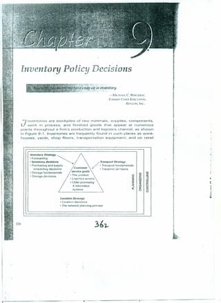
1. Inventory Policu Decisions
l1 .~~~ ,'f.~·~'~I~~"':'r::,
_
,I',.0 '. •
~viiK~,j2~~{s
ttk'ln ihvel1toYIj.
~:il~~ti'~*,;
~,',"/'fI.{.l :':,..' .;.; ,I,
-MICHM,L C. BER(;ERAC
FORMEI? 0 liEF EXECUTIVE.
REVLON, INc.
J
nventories are stockpiles of raw materials, supplies, components,
work in process, and finished goods that appear at numerous
points throughout a firm's production and logistics channel, as shown
in Figure 9-1. Inventories are frequently found in such places as ware-
houses, yards, shop floors, transportation equipment, and on retail
Inventory Strategy /
• Forecasting ~
• Inventory decisions ~ / Transport Strategy
• Purchasing and supply • Transport fundamentals
scheduling decisions Customer I • Transport decisions
• Storage fundamentals service goals
e CI
• Storage decisions • The product CI Z ,2:
/ • Lopistics "~,,,
z !Si
::i
2
..J
• Order processing Z 0
2 « a:
& information « c"
I-
..J
a: Z
systems
D-
O 0
o
Location Strai'egy
• Location decisions
• The network planning process
- -
-
..
c
(
I
t
jj
326

2. _.i :J (J) :'
"
• __ ._:"'&"" .•••••• ,... w.
V>
tr-;
Vl
f.U
N
~
Material
sources
Inbound
transportation
Figure 9-1 Inventories Are Located at Each Echelon of the Supply Channel
;---~----------i
r. ~:.~ . _~ :
~ .• '.!! IY,
, CIl . ,
./', g Production ,
~/!~;:
i
: . V
,
C>
v Inventory
locations
'.-:==-'~---'-----
Production Outbound
transportation
Finished
goods
warehousing
Customers
Inventories
in-pr~cess
e,J'tl~~
~(~
,,,
,
i /~
i!lJi.,,[(~ ~"'_.
d .e-, V
Finishe s: , .,
Ul, .,.
goods ,
1_-- .J

3. store shelves. Having these inventories on hand can cost betvveen 20
and 40 percent of their value per year. Therefore, carefully managing
inventory levels makes good economic sense. Even though many
strides have been taken to reduce inventories through just-in-time, time
compression, quick response, and collaborative practices applied
throughout the supply channel, the annual investment in inventories by
manufacturers, retailers, and merchant V{holesalers,vvhose sales repre-
sent about 99 percent of GNP, is about 12 percent of the U.S. gross
domestic product." This chapter is directed tovvard managing the inven-
tories that remain in the supply channel.
There is much to learn about inventory management and this chap-
ter is rather lengthy because of it; hovvever,the subject can be vievved
in three major parts. First, inventories are most frequently managed as
individual items located at single stocking points. This inventor:y con-
trol type has been researched extensively vvith methods for many spe-
cific applfcations. Second, inventory control vvill be vievved as manage-
ment of inventory in the aggregate. Top managers are particularly
interested in this perspective because of their need to control the over-
all inventory investment rather than individual stock-keeping units.
Finally, m'anaging inventories among multiple locations and multiple
echelons vvithin the supply channel vvill be examined.
ApPRAISAL OF INVENTORIES
There are numerous reasons why inventories are present in a supply channel, yet in
recent years inventory holding has been roundly criticized as unnecessary and
wasteful. Consider why a firm might want inventories at some level in its operations,
and why that firm would want to keep them to a minimum.
Arguments for Inventories
Reasons for holding inventories relate to customer service or to cost economies indi-
rectly derived from them. Briefly consider some of these.
Improve Customer Service
Operating systems may not be designed to respond to customer requests for product
or services in an instantaneous manner. Inventories provide a level of product or ser-
vice availability, which, when located in the proximity of the customer, can meet high
customer expectations for product availability. The availability of these inventories
to customers can not only maintain sales, but they can also increase them.
1U.S. Bureau of the Census, Statistical Abstract of the United States.' 2001. 121 th ed. (Washington, DC: 2001),
pp. 623, 644, and 657. •
328 Part IV Inventory Strategy
Applicc'
Auto repai
of automol
To provide
popular pa
maintains i
transportee
the same d
with a mini
Reduce c.
Although h
operating c
inventory Ci
duction by i
put can be e
exist to act a
Second,
Apurchasin
in order to r.
until theyar
similar maru
quantities th
causes incres
portation ch
inventory.
Third, h
lower curren
ti ties greater
in quantities
expected to r
justified.
Fourth, '
throughout I
costs as well
points in the
smooth opere
Fifth, unF
strikes, natur
conlingencie~
inventory at ~
for a period VI

4. ~':.Il20
laging
many
.I •• time
IPI)lied"
,if,3s by
repre-
gross
inven-
, chap-
iiewed
oed as
,
~ycon-
lY spe-
pnage-
G~arly
l~ over-
, units.
.ult ip le
1'1,yel in
sary ~and
.erations.
nics incli-
r product
Jet or ser-
-ncet high
Iventories
,DC: 2001),
Application
Auto repair shops are faced with maintaining thousands of repair parts for a variety
of automobiles from different model years. An automobile can contain 15,000 parts.
To provide the fastest turnaround, repair shops carry a limited inventory of the more
popular parts such as spark plugs, fan belts, and batteries. The auto manufacturer
maintains a second inventor), tier.in regional warehouses from which parts can be
transported using airfreight. The repair shops can, in some cases, receive these parts
the same day they me requested. t.high level of parts availability can be achieved
with a minimum of on-site inventory.
,
i
I
I
.1
I
I
I
Reduce Costs
Although holding inventories has an associated cost, their use can indirectly reduce
operating costs in other supply channel activities that may more than offset the
inventory carrying cost. First, holding inventories may encourage economies of pro-
duction by allowing larger, longer, and more level production runs. Production out-
put can be decoupled from the variation in demand requirements when inventories
exist to act as buffers between the two. •
Second, holding inventories fosters economies in purchasing and transportation.
A purchasing department may buy in quantities beyond the firm's immediate needs
in order to realize price-quantity discounts. The cost of holding the excess quantities
until they are needed is balanced with the price reduction that can be achieved. In a
similar manner, transportation costs can often be reduced through shipping in larger
quantities that require less handling per unit. However, increasing the shipment size
causes increased inventory levels that need to be maintained at bon: ends of the trans-
portation channel. The reduction in transportation costs justifies the carrying of an
inventory.
Third, forward buying involves purchasing additional product quantities at
lower current prices rather than at higher anticipated future prices. Buying in quan-
tities greater than immediate needs causes a larger inventory than does purchasing
in quantities that more closely match immediate requirements. However, if prices are
expected to rise in the future. some inventory resulting from forward buying can be
justified.
Fourth, variability in the time that it takes to produce and transport goods
throughout the supply channel can cause uncertainties that impact on operating
costs as well as customer service levels. Inventories are frequently used at many
points in the channel to buffer the effects of this variability and, thereby, help to
smooth operations.
Fifth, unplanned and unanticipated shocks can befall the logistics system. Labor
strikes, natural disasters, surges in demand, and delays in supplies are the types of
contingencies against which inventories can afford some protection. Having some
inventory at key points throughout the supply channel allows the system to operate
for a period while the effect of the shock can be diminished.
i
I
I
Chapter 9 Inventory PolicyDecisions 329

5. Application
Papermaking requires expensive Fourdrinier machines and other pieces of equip-
ment that have large capacities. The high fixed cost of this equipment dictates that it
constantly be kept busy. Demand for industrial paper products (e.g., kraft wrapping
papers, multiwall bags, and bulk products) is anything but stable and known for
sure. Although large orders can be scheduled directly to the process, production of
small orders 'would be too costly, considering that changeovers can take -SOminutes
on machines costing $3,500 per hour to operate. Producing to an inventory and
servicing the small-order demand for the more standardized products from
that inventory reduces setup time, which more than compensates for the inventory-
carrying cost.
Arguments Against Inventories
It has been claimed that management's job is much easier having the security of
inventories. Being overstocked is much more defensible from criticism than being
short of supplies. The major portion of inventory-carrying costs is of an opportunity
cost nature and, therefore, goes unidentified in normal accounting reports. To the
extent that inventory levels have been too high for the reasonable support of opera-
tions, the criticism is perhaps deserved.
Critics have challenged the holding of inventories along several lines. First,
inventories are considered wasteful. They absorb capital that might otherwise be
put to better use, such as to improve productivity or competitiveness. In addition,
they do not contribute any direct value to the firm's products, although they do
store value.
Second, they can mask quality problems. When quality problems occur, reducing
existing inventories to protect the capital investment is often a first consideration.
Correcting quality probfems can be slow.
Finally, using inventories promotes an insular attitude about the management of
the supply channel as a whole. With inventories, it is often possible to isolate one
stage of the channel from another. The opportunities arising from integrated decision
making that considers the entire channel are not encouraged. Without inventories, it
is difficult to avoid planning and coordinating across several echelons of the channel
at one time.
TYPES OF INVENTORIES
330
Inventories can be categorized in five distinct forms. First, inventories may be in the
pipeline. These are inventories in transit between echelons of the supply channel.
Where movement is slow and/ or over long distances, or movement must take place
between many echelons, the amount of inventory in the pipeline may well exceed
that held at the stocking points. Similarly, work-in-process inventories between man-
ufacturing operations can be considered as inventories in the pipeline.
'.2i66
Part IV Inventory Strategy
Second, ~
inven tory ba
are purchase
merits. Wher
of operation:
management
antiCipation
inventories a
Third, sf
sary to meet
merits. The <L
nornical ship
price-quantit
Fourth, i_
for the inven
or safety stoe
demand anc
statistical pn
The amount
ability involx
casting is es
demand COLI:
needed.
Finally, s
stolen when}
stock. Where
cautions mus
CLASSIFYI"
MANAGEM
Managing inv
ries cannot bt
methods intc
methods wiII
Chapter 10. V
the cond ition:
inventory-reI;
control, givel
directly to del-
ity in demand
relationships
accurate ordei

6. if pquip-
'5~that i~
IC<lpping
iown for
uction of
"minutes
lory and
~ls from
.ventory-
hUl~ily of
an being
)ortunily
s. To the
~.Ifopera-
es, First,
l'Wise be
itddilion,
ithey <..10
rcdlfcing
deration.
.ernerit of
olate one
Idecision
ntories, it
e channel
-be in the
. cll..~nnel.
take place
211exceed
I Second, some stocks may be held for speculation, but they are still part of the total
inventory base that must be managed. Raw materials such as copper, gold, and silver
are purchased as much for price speculation as they are to meet operating require-
ments. Where price speculation takes place (or periods beyond the foreseeable needs
of operations, such resulting inventories are probably more the concern of financial
management than logistics management. However, when inventories are built up in
anticipation of seasonal selling or occur due to forward buying activities, these
inventories are likely to be the responsibility of logistics.
Third, stocks may be regutar or cyclical in nature. These are the inventories neces-
sary to 'meet the average demand during the timebetween successive replenish-
ments. The amount of cycle stock is highly dependent on production lot sizes, eco-
nomical shipment quantities, storage space limitations, replenishment lead times,
price-quantity discount schedules, and inventory carrying costs.
Fourth, inventory may be created as a hedge against the variability in demand
for the inventory and in replenishment lead time. This extra measure of inventory,
or safety stock, is in addition to the regular stock that is needed to meet average
demand and" average lead-time conditions. Safety stock.is determined. from
statistical procedures that deal with the random nature of the variability involved.
The amount of safety stock maintained depends on the extent of the vari-
ability involved and the level of stock availability that is provided. Accurate fore-
casting is essential to minimizing safety stock levels. In fact, if lead time and
demand could be predicted with 100 percent accuracy, no safety stock would be
needed.
Finally, some of the inventory deteriorates, becomes out of date, or is lost or
stolen when held for a time. Such inventory is referred to as obsolete, dead, or shriilknge
stock. Where the products are of high value, perishable, or easily stolen, special-pre-
cautions must be taken lo rrunimize the amount of such stock.
CLASSIFYING INVENTORY
MANAGEMENT PROBLEMS
Managing inventories involves a variety of problem types. Since managing invento-
ries cannot be handled using a single solution method, we need to categorize the
methods into several major groups. Inventory management using just-in-time
methods will not be included in this f,wuping, since the technique is discussed in
Chapter 10. Witll the remaining inventory management methods, we assume that
the conditions of demand level and its variability, lead time and its variability, and
inventory-related costs are known, and that we must do the best job of inventory
control, given these conditions. In contrast, the just-in-time philosophy (supply
directly to demand as it occurs) is to eliminate inventories by reducing the variabil-
ity in demand and replenishment cycle time, reducing lot sizes, and forging strong
relationships with a limited number of suppliers to ensure quality products and
accurate order filling.
367, Chapter 9 Inventory Policy Decisions 331

7. Nature of Demand
,.
The nature of demand over time plays a significant role in determining how we treat
the control' of inventory levels. Several common types of demand patterns are shown
in Pigure 9-2. Perhaps the most common demand characteristic is for it to continue
into the indefinite future. The demand pattern is referred to as perpetual. Although
demand for most products rises and falls through their life cycles, many products
have a selling life that is sufficiently long to be considered infinite for planning pur-
poses. Even though brands turn over at the rate of 20 percent per year, a life cycle of
three to five years can be long enough to justify treating them as having a perpetual
demand pattern.
On the other hand, some products are highly seasonal or have a one-time, or
spike, demand pattern. Inventories that are heJd to meet such a demand pattern usu-
ally cannot be sold off without deep price discounting. A single inventory replenish-
ment order must be placed with little or no opportunity to reorder or return goods if
demand has been inaccurately projected. Fashion clothing, Christmas trees, and
political campaign buttons are examples of this type of demand pattern.
Similarly, demand may display a lumpy, or erratic, pattern. The demand may be
perpetual, but there are periods of little or no demand followed by periods of high
demand. The timing of lumpy demand is not as predictable as for seasonal demand,
which usually occurs at the same time every year. Items in inventory are typically a
mixture of lumpy and perpetual demand items. A reasonable test to separate these is to
recognize that lumpy items have a high variance around their mean demand level. If
the standard deviation of thedemand distribution, or the forecast error, is greater than
Figure 9-2
Examples of
Common
Product Demand
Patterns
/' Terminating-
...,,!" aircraft parts
......
...... .....
..
. .
•....:. '.:
U)
•..
'c
:>
-c
c
E Lumpy-
~ construction
eQuiPment7
11
I I
: I
.....
rS~;~~n::~
....... conditioners
• A
'. 1
'. I I
• I I
;. '.. "
" ', •••. I '.
I I-
I • I
~,
~
'I
I,
I
I
I
I
I I
I ,
I
I
I
...•.•...... I
"
, ,
I ,
,
Time
332 Part IV Inventory Strategy
the averag
items is be:
proceduret
There
future, wh
raining inv
the limited
mili tary ail
ucts with a
perpetual I
products (c
Finally
other item.
primary pi
handled wi
cussed in (
Manager
Inventory I
the pull api
house, as n
mining rep
conditions,
Figure 9-3
Pull Versus Pl
Inventory
Management
Philosophies

8. we treat
'~shown
continGe
~lthough
products
ling pur-
r cycle of
JerpctuaJ
<time. or
tern u u-
'Cplcl,ish-
1 goods if
rees, and
d may be
Is of high
demand,
ypically <I
these is to
d level. If
eater than
isonal-e-
orn air
ditioners
---
the average demand, or forecast, the item is probably lumpy. Inventory control of such
items is best handled by intuitive procedures, or by a modification of the mathematical
procedures discussed in this chapter. or through collaborative forecasting.
There are products whose demand terminates at some predictable time in the
future, which is usually longer than one year. Inventory planning here involves main-
taining inventories to just meet demand requirements, but some reordering within
the limited time horizon is allowed. Textbooks with planned revisions, spare parts for
military aircraft, and pharmaceuticals with a limited shelf life are examples of prod-
ucts with a defined life. Since the distinction. between these products and those with a
perpetual life is often blurred, they will not be treated differently from perpetual-life
products for the purposes of developing a methodology to control them.
Finally, the demand pattern for an item may be derived from demand for some
other item. The demand for packaging materials is derived from the demand for the
primary product. The inventory control of such dependent demand items is best
handled with some form of just-in-time planning such as MRP ~r DRP, which are dis-
cussed in Chapter 10.
Management Philosophy
Inventory management is developed around two basic philosophies. First, there is
the pull approach. This philosophy views each stocking point, for example, a ware-
house, as independent of all others in the channel. Forecasting demand and deter-
mining replenishment quantities are accomplished by taking into account only local
conditions, as illustrated in Figure 9-3. No direct consideration is given to the effect.
Figure 9-3
Pull Versus Push
Inventory
Management
Philosophies
Push-Allocate supply to each
warehouse based on the
forecast for each warohouse
Pull-Replenish inventory with
order sizes based on specific
needs of each warehouse
Demand
forecast
01 Warehouse #1
Demand
forecast
Warehouse #2
A = Allocation quantity to each ~ ~
warehouse. Warehouse #3
n = Requested replenishment
uuanritv by each warehouse
Demand
forecast
36~. I Chapter 9 Inventory Policy Decisions 333
j

9. that the replenishment quantities, each with thei'f different levels and timing, will
have on the economics of the sourcing plant. However, this approach does give pre-
cise control ,over inventory levels at each location. Pull methods are particularly pop-
ular at the retail level in the supply channel where over 60 percent of the hard goods
and almost 40 percent of the soft goods are under replenishment programs.?
Alternatively, there is the push approach to.inventory management (see Figure 9-3).
When decisions about each inventory are made independently, the timing and replen-
ishment order sizes are not necessarily well coordinated with production lot sizes,
economical purchase quantities, or order size minimums. Therefore, many firms choose
to allocate replenishment quantities to inventories based on projected needs for inven-
tories at each location, available space, or some other criteria. Inventory levels are
set collectively across the entire warehousing system. Typically, the push method is
used when purchasing or production economies of scale outweigh the benefits of
minimum collective inventory levels as achieved by the pull method. In addition,
inventories can be managed centrally for better overall control, production and pur-
chase economies can be used to dictate inventory levels for lower costs, and forecasting
can be made on aggregate demand and then apportioned to each stocking point for
improved accuracy. .
Collaborative replenishment can be used as a hybrid of the pull and push meth-
ods. In this case, the channel members representing the source point and the stocking
point jointly agree on the replenishment quantities and their timing. The result can.
be order replenishment that is more economical for the supply channel than if either
party alone were to make the replenishment decision.
Degree of Product Aggregation
Much of inventory control is directed at controlling each item in inventory. Precise
control of each item can lead to precise control of the sum of all item inventory levels.
This is a bottoms-up approach to inventory management.
Management of product groups rather than individual items is an alternate, or
top-down, approach-a common perspective of top management. Although dairy
operation of inventories may require item-level control, strategic planning of inven-
tory levels can be accomplished by substantially aggregating products into broad
groups. This is a saijsfactory approach when managing the inventory investment of
all items collectively is the issue, and the effort associated with an item-by-item
analysis for thousands of items at many 'locations is not warranted. Methods of
control tend to be less precise for aggregate inventory management than for item
management.
Multi-Echelon Inventories
As supply chain management has encouraged managers to think about including
increasingly more of the supply channel in their planning processes, inventories that
334
2'fom Andel, "Manage Inventory, Own Information," Transportation & Distribution (May 1996), p. 54ff.
.~
370'
Part [V Inventory Strategy
span mo
ries at eY
overall i:
larly diff
to manaj
Virtual
Historic.
assigned
on back,
firms to
work, CTI
could be
when cre
product:
INVENTC
Inventor
on the OJ
the other
get, we 1
(see Figc
tories wi
evant to
Figure
Design C
inventor,

10. u~ng, will
~give pre-
Ja£lypop-
Ilra goods
,"'2 ' }'
h
',igure9-3).
,'Id replen-
('lot sizes,
n5. choose
for inven-
levels are
method is
)en..
efits of
"addition,
and pur-
:()n~casting
; point for
ush rneth-
.e stocking
result can,
In if either
IIY ~recise
.ory levels.
lema ie, or
JLlglf dairy
b of inven-
into broad
estment of
in-by-item
Iethods of
111 for item
t including
ntories that
6), p, 54ff.
:,
span more than one channel echelon become a focus. Rather than planning invento-
ries at each location separately, planning their levels in concert can lead to lower
overall inventory quantities. Multi-echelon inventory planning has been a particu-
larly difficult problem to solve, but some progress is being made in methods useful
to managers.
Virtual Inventories
Historically, customers have been served from inventories to which they were
assigned. If product was out of stock, either a sate was lost or the product was placed
on back order. Improved information systems changed that. It became possible for
firms to know product inventory levels at every stocking point in the logistics net-
work, creating a virtual inventory of products. Because of':his, out-of-stock items
could be replaced by cross filling them from' other locations. Satisfying demand
when cross filling is an option can result in lower overall inventory levels and higher
product fill rates.
INVENTORY OBJECTIVtS
Inventory management involves balancing product availability, or customer service,
on the one hand with the COBts
of providing a given level of product availability on
the other. Since there may be more than one way of meeting the customer service tar-
get, we seek to minimize inventory-related costs for each level of customer service
(see Figure 9-4)0 Let us begin the development of the methodology to control inven-
tories with a way to define product availability and an identification of the costs rel-
evant to managing inventory levels. 0
Figure 9-4
Design Curves for
Inventory Planning
~-----"----------------------------------------,
High
it.. ,Minimum
cost curve
A Alternate stocking plans
..,
'"
o
o
e
o
C
<Il
>
C
Low _A,==='-- --'- ---' 0
Low Product availability High
100%,
OJ:;
c=
':0
'Ill
.c
o
0..
.:.:
o
o
..,
'"
C:
Chapter 9 Inventory PolicyDecisions 335
:;71

11. Product Availability
A primary objective of inventory management is to ensure that product is available
at the time and in the quantities desired. This is commonly judged based on' the prob-
ability of fulfillment capability from current stock. This probability, or item fill rate, is
referred to as the service level, and, for a single item, can be defined as
Expected number
S
. I I 1 of units out of stock annuallv
ervlce eve = - ----------....:....
Total annual demand
(9-11
. ,
Service level is expressed as a value between 0 and 1. Since a target service level is
typically specified, our task will be to control the expected number of stock out units.
We will see that controlling the service level for single items is computationally
convenient. However, customers frequently request more than one item at a time.
Therefore; the probability of filling the customer order completely can be of greater
concern than single-item service levels. For example, suppose that five items are
requested on an order where each item has a fill rate of 0.95, that is, only a 5 percent
chance of not being in stock. Filling the entire order without any item being out of
stock would be
0.95 x 0.95 x 0.9,5 x 0.95 x 0.95 = 0.77
The probability of filling the order completely is somewhat less than the individual
item probabilities.
A number of orders from many customers will show that a mixture of items can
appear on anyone order. The service level is then more properly expressed as
a weighted average fill rate (WAFR). The WAFR is found by multiplying the frequency
with which each combination of items appears on the order by the probability of filling
the order completely, given the number of items on the order. If a target WAFR is spec-
ified, then the fill rates for each item must be adjusted to achieve this desired WAFR.
Example
A specialty chemical company receives orders for one of its paint products. The paint
product line contains three separate items that customers order in various combina-
tions. From a sampling of orders over time, the items appear on orders in seven dif-
ferent combinations wfth frequencies as noted-in Table 9-1. Also from the company's
historical records, the probability of having each item in stock is SLA' = 0.95; 5LB
=
0.90; and SLc = 0.80. As the calculations in Table 9-1 show, the WAFR is 0.801. There
will be about one order in five where the company cannot supply all items at the time
of the customer request.
Recall that additional measures for customer service were discussed in Chapter 4.
Some of these measures encompass more than inventory and are not appropriate for
336 Part IV Inventory Strategy 312.
ITEM Cosnn
ONORDEf
A
B'
C
A, B
A,e
B,e
A,B,C
Table 9-1
the disc
include
orders f
second a
t
Releva
Three gE
curernen
trade-off
inventor
Figure
Trade-Oft
Relevant
Costs wit
Quantity

12. .ailable
.cprob-
l.r!te, isp
(9-1)
level is
It units.
llO! ally
a time.
greater
uns are
percent
~out of
[vidual
omscan
ssed as
~quency
.f fill' 19
isspec-
IAFR
ie paint
nnbina-
ven dif-
rpany's
; 5LH =
l. There
he time
.apter 4.
riate for
r '.
ll"EM COMBINATION (1) FREQUfNCY (2) PROBABILITY OF FILLING (3) = (1) x (2)
ONORDEII UFORlJlm ORDER COMPLETE MARGiNAL VALUE
A 0.1 (.95) = 0.950 0.095
B' 0.1 (.90) = 0.900 0.090
C 0.2 (.80) = 0.800 0.160
A,B. 02 (.95)(.90) = 0.855 0.171
A,C 0.1 (.95)(.80) = 0.760 0.076
B,C OJ (.90)(.80) = 0.720 0.072
A,B,e 0.2 (.95)(.90)(.80) = 0.684 0.137
-- --
1.0 WAFR= 0.801
-
Table 9-' Computation of the Weighted Average Fill Rate
the discussion here. However, additional inventory performance measures might
include percent of items on back order, percent. of orders filled complete, percent of
orders filled complete to a given percentage, and percent of items cross filled from
secondary locations. These are not discussed further.
Relevant Costs
Three general classes of costs are important to determining inventory policy: pro-
curement costs, carrying costs, and stockout costs. These costs are in conflict, or in
trade-off, with each other. For determining the order quantity to replenish an item in
inventory, these relevant costs trade-off are shown in Figure 9-5.
Figure 9-5
Trade-Off of the .
Relevant Inventory
Costs with the Order
Quantity
Carrying
costs
VI
1;;
o
u
C
<1:
>
Q)
e
Q*
Quantity ordered, Q
Chapter 9 Inventory Policy Decisions 337

13. ,.
Procurement Costs
Costs associated with the acquisition of goods for the inventory replenishment are often
a significant economic force that determines the reorder quantities. When a stock replen-
ishment order is placed, a number of costs are incurred that are related to the processing,
setup, transmitting, handling, and purchase of the order. More specifically, procurement
costs may include the price, or manufacturing cost, of the product for various order sizes;
the cost for setting up the production process; the cost of processing an order through the
accounting and purchasing departments; the cost of transmitting the order to the supply
point, usually using mail or electronic means; the cost of transporting the order when
transportation charges are not included in the price of the purchased goods; and the cost
of any materials handling or processing of the goods at the receiving point. When the
firm is self-supplied, as in the case of a factory replenishing its own finished goods inven-
tories, procurement costs are altered to reflect production setup costs. Transportation
costs may not be relevant if a delivered pricing policy is in effect.
Some of these procurement costs are fixed per order and do not vary with the order
size. Others, such as transportation, manufacturing, and materials-handling costs, vary
to a degree with order size. Each requires slightly different analytical treatment.
Carrying Costs
Inventory carrying costs result from storing, or holding, goods for a period and are
roughly proportional to the average quantity of goods on hand. These costs can be
collected into four classes: space costs, capital costs, inventory service costs, and
inventory risk costs.
Space Costs. Space costs are charges made for the use of the volume inside the stor-
age building. When the space is rented, storage rates are typically charged by weight
for 'a period of time, for example, $/cwt./month. If the space is privately owned or
contracted, space costs are determined by allocating space-related operating costs,
such as heat and light, as well as fixed costs, such as building and storage equipment
costs, on a volume-stored basis. Space costs are irrelevant when calculating carrying
costs for in-transit inventories.
Capital Costs. Capital costs refer to the cost of the money tied up in inventory. This
cost may represent over 80 percent of total inventory cost (see Table 9-2), yet it is the
most intangible and subjective of all the carrying cost-elements. There are two rea-
..sons for this. First, inventory represents a mixture -of short-term and long-term
assets, as some stocks may serve seasonal needs and others are held to meet longer-
term demand patterns: Second, the cost of capital may vary from the prime rate of
interest to the opportunity cost of capital.
The exact cost of ~apit{ll for inventory purposes has been debated for some time.
Many firms use their average cost of capital, whereas others use the average rate of
return required of company investments. The hurdle rate has been suggested as most
accurately reflecting the true capital cost.3 The hurdle rate is the rate of return on the
most lucrative investments that the firm does not accept.
3Douglas M, Lambert and Bernard J, LaLonde, "Inventory Carrying Costs," Management Accollntitrg
(August 1976), pp. 3]-35.
338 Part IV Inventory Strategy
Tabl
Relat.
of Co:
Inven
Costs
Inventory
costs bec',
Insurance
Inventory
Although
reflects th
represent
from acco
Inventory
age, or ob
maintaini:
damaged,
ciated witl
of reworki
.
om-a-s
Out-of-sto
inventory
stock cost!
the part 01
measure a
A lost
chooses tc
. would hai
the negan-
customer :~
soft drink!
Aback
so that tlu
and sales
costs whei
costs are t,

14. Ire often
:replen-
cossing,
• (';I
iremenf
lersizes;
J!lgh the
~supply
~r when
the cost
(hen the
lsinven-
ortation
he order
'!
sts, vary
.
and are
5 can be
sts, and
the stor-
{weight
wned or
19 costs,
uipdtent
carrying
ory. This
t it is the
two rea-
.ng-term
t longer-
re rate of
me time.
;e rale of
j as most
rn en the
IIIlil1S
Table 9-2
Relative Percentages
of Cost Elements in
Inventory Carrying
Costs
Interest and opportunity costs
Obsolescence and physical depreciation
Storage and handling
Property taxes
Insurance
Total
82.00%
14.00
3.25
0.50
0.45
100.00%
Sown': Adapted from Robert Landeros and David M. Lyth,
"Economic- Lot-Size Models for Cooperative Inter-Organizational
Rt-lationshipR," [ourno! of Busilless logistics, Vol. 10, No.2 (1989),
p.14Q. II
Inventory Service Costs. Insurance and taxes are also a part of inventory carrying
costs because their level roughly depends on the amount of inventory on hand.
Insurance coverage is carried us a protection against losses from fire, storm, or theft.
Inventory taxes are levied on the inventory levels found on the day of assessment.
Although the inventory at the point in time of the tax assessment only crudely
reflects the average inventory level experienced throughout the year, taxes typically
represent only a small portion of total carrying cost. Tax rates are readily available
from accounting or public records. '
Inventory Risk Costs. Costs associated with deterioration, shrinkage (theft), dam-
age, or obsolescence make up the final category of carrying costs. In the course of
maintaining inventories, a certain portion of the stock will become contaminated,
damaged, spoiled, pilfered, or otherwise unfit or unavailable for sale. The costs asso-
ciated with such stock m<tybe estimated as the direct loss of product value, as the cost
of reworking the product, or as the cost of supplying it from asecondary location.
Out-oF-Stock Costs
Out-of-stock costs are incurred when an order is placed but cannot be filled from the
inventory to which the order is normally assigned. There are two kinds of out-of-
stock costs: lost sales costs and back order costs. Each presupposes certain actions on
the part of the customer, and, because of their intangible nature, they are difficult to
measure accurately.
A lost sales cost occurs when the customer, faced with an out-of-stock situation,
chooses to withdraw his or her request for the product. The cost is the profit, that
. would have been made on this particular sale and may include an additional cost for
the negative effect that the stockout may have on future sales. Products for which the
customer is very willing to substitute competing brands, such as bread, gasoline, or
soft drinks, are those that are most likely to incur lost sales.
A back order cost occurs when a customer will wait for his or her order to be filled
so that the sale is not lost, only delayed. Back orders can create additional clerical
and sales costs for order processing, and additional transportation and handling
costs when such orders are not filled through the normal distribution channel. These
costs are tangible, so measurement of them is not too difficult. There also may be the
3'(
Chapter 9 Inventory Policy Decisions' 339

15. intangible cost of lost future sales. This cost is very difficult to measure. Products
(automobiles and major appliances) that can be differentiated in the consumer's
mind are more likely to be back ordered than substituted.
PUSH INVENTORY CONTROL
Let's begin to develop methods for controlling inventory levels with the push philos-
ophy. Recall that this method is appropriate where production or purchase quantities
exceed the short-term requirements of the inventories into which the quantities are to
be shipped. If these quantities cannot be stored at the production site for Jack of
space or other reasons, then they must be allocated to the stocking points, hopefully
in some way that makes good economic sense. Push is also a reasonable approach to
inventory control where production or purchasing is the dominant force in deter-
mining the replenishment quantities in t,he channel. In either case, the following
questions need to be addressed. How much inventory should be maintained at each
stocking point? How much of a purchase order or production run should be allo-
cated to each stocking point? How should the excess supply over requirements be
apportioned among the stocking points?
A method for pushing quantities into stocking points involves the following steps:
1. Determine through forecasting or other means the requirements-for the period
between now and the next expected production run or vendor purchase.
2. Find the current on-hand quantities at each stocking point.
3. Establish the stock availability level at each stocking point.
4. Calculate total requirements from the forecast plus additional quantities needed
to cover uncertainty in the demand forecast.
5. Determine net requirements as the difference between total requirements and
the quantities on hand.
6. Apportion the excess over total net requirements to the stocking points on the
basis of the average demand rate, that is, the forecasted demand.
7. Sum the net requirements and prorate the excess quantities to 'find the amount
to be allocated to each stocking point.
Example
When the tuna boats are sent to the fishing grounds, a packer of tuna products must
process all the tuna caught since storage is limited and, for competitive reasons, the
company does not want to sell the excess of this valued product to other packers.
Therefore, this packer processes all fish brought in by the fleet 'and then allocates the
production to its three field warehouses on a monthly basis. There is only enough
storage at the plant for one month's demand. The current production ruri is 125,000 lb.
For the upcoming month, the needs of each warehouse were forecasted, the cur-
rent stock levels checked, and desired stock availability level noted for each ware-
house. The findings are tabulated in Table 9-3.
340 Part IV Inventory Strategy
WAREIIOUSE c
1
2
3
'Assumed to be nom
!>Stock availability leI
Table 9-3 B
Now I
. ~
regUlJ'eme
needed to
where z is
beyond the
under the I
in Append
(1.28 X 2,01
The inform
Net rec
quantity I
that 125,001
rated to the
I
II
I
I
Figure 9·
Area Under
Forecast Dis
for Warehol

16. ~rodllcts
li~sumer's
,j?
~J"philos-
quantities
ities are to
[or lack of
hopefully
}p.roach to
e in deter-
following
Ij:!d at each
Id be allo-
'~ments be
ving steps:
IC period
se.
.es needed
-nts and
:
.s on the
. amount
ducts must
easons the
er packers.
lloca tes the
ily enough
.125,000 lb.
zd. the cur-
each ware-
FORECAsrFD DEMAND
FORECAST ERROR"
(STD. DEV.}
STOCK AVAlLADlUTY
LEVELb
Now we need to compute the total requirements for each warehouse. Total
requirements for warehouse 1 will be the forecast quantity and the added amount
needed to ensure a 90 percent stock availability level. This is found from
Total requirements = Forecast + (z x Forecast error)
where z is the number of standard deviations on the normal distribution curve
beyond the forecast (the distribution mean) to the point where 90 percent of the area
under the curve is represented (see Figure 9-6). From the normal distribution curve
in Appendix A, z = 1.28. Hence, the total requirement for warehouse 1 is 10,000 +
(1.28 X 2,000) = 12,560. Other warehouse total requirements are computed similarly.
The information is recorded in Table 9-4.
Net requirements are found as the difference between total requirements and the
quantity on hand in the warehouse. Summing the net requirements (110,635) shows'
that 125,000 - 110,635 = 14,365, which is the excess production that needs to be pro-
rated to the warehouses.
Chapter 9 Inventory Policy Decisions 341
WAREHOUSE CURReNT STOCK LEVEl
5,0001b
15,000
30,000
1O,0001b
50,000
70,000
130,000
2,0001b
1,500
20,000
1
2
3
90%
95%
90%
'Assumed to be normally distributed,
"stock availability level is d,efined as the probnbility of stock being available during the forecast period.
Table 9-3 Basic Inventory Planning DAta for a Tuna Packer
Figure 9-6
Area Under the
Forecast Distribution
for Warehouse 1
90% of area
under curve
Forecasted demand'
':" 10,000 Ib
Total requirement
= 12,560 Ib

17. (1) TarAL (2) (3) = (1) - (2) (4) PRORATED (5) = (3) + (4)
.t
WAREHOUSE REQUIREMENTS ON HAND NET REQUIREMENTS EXCESS ALLOCATION
The per
1 12,5601b 5,000 7,5601b 1,1051b 8,6651b
". 2 52,475 15,000 37,475 5,525 43,000
3 95,600 30,000 65,600 7,735 73,335 Considr
,
its and I
160,635 110,635 14,365 125,000
Table 9-4 Allocation of Tuna Production to Three Warehouses
where C
uct. SolI
Prorating the excess production of 14,3651b is made in proportion to the average
demand rate for each warehouse. Average demand for warehouse 1 is 10,000 Jb
against a total demand rate for all warehouses of ]30,000 lb. The proportion of the
excess allocated to warehouse 1 should be (10,000 + 130,000)(14,365) = 1,105. Prorate
the excess for the remaining warehouses in a similar manner. The total allocation to a
warehouse is the sum of its net requirement plus its portion of the production excess.
The results are tabulated in Table 9-4.
BASIC PULL INVENTORY CONTROL
Recall that pull inventory control gives low inventory levels at stocking points
because of its response to the demand and cost conditions particular to each stocking
point. Although many specific methods have been developed to handle a variety of
situations, the discussion here will attempt to highlight the fundamental ideas.
Specifically, a contrast will be.made between (1) demand that is one-time, highly sea-
sonal, or perpetual; (2) ordering that is triggered from a particular inventory level or
from a process of inventory level review; and (3) the degree of uncertainty in
demand and replenishment lead time.
Single-Order Quantity
Many practical inventory problems exist where the products involved are perishable
or the demand for them is a one-time event. Products such as fresh fruits and vegeta-
bles, cut flowers, newspapers, and some pharmaceuticals have a short and defined
shelf life, and they are not available for subsequent selling periods. Others, such as
toys and fashion clothes for the immediate selling season, hotdog buns for a baseball
game, and posters for a political campaign, have a one-time demand level that usually
cannot be estimated with certainty. Only one order can be placed for these products to
meet such demand ..We wish to determine how large the single order should be.
To find the moss economic order size (Q*), we can appeal to marginal economic
analysis. That is, Q* is found at the point where the marginal profit on the next unit
sold equals the marginal loss of not selling the next unit. The marginal profit per unit
obtained by selling a unit is
342 Part IV Inventory Strategy
This say
probabi
Exan
AgroceJ
salad in
dard de'
It pays:
unsold E
Fine
comp~h
From th
of 58.3 p
0.21. ThE
wi«-
such cas
Exarr
An equi]
running

18. "--,
; 3) + (4)
II.OCATION
~651b
, OJ'
p,OOO
~3,335
;'5,00(1
he average
s 1),000 Ib
rtion of the
:US. Prorate
.,lca1.ionto a
lion excess.
,ing points
ch stocking
a variety of
en La] ideas.
.highly sea-
ory level or
:ertainty in
e perishable
and vegeta-
and defined
icrs, such as
)1' a basebal I
that usually
~prod ucts 1:0
ulJ be.
tal economic
.he next uni t
rofrt per unit
Profit = Price per unit - Cost per unit
The per-unit Joss incurred by not selling a unit is
Loss = Cost per unlt - Salvage value per unit
(9-2)
(9-3)
Considering the probability of a given number of units being sold, the expected prof-
its and losses are balanced at this point. That is, II
ePn (Loss) = (1 - CPn)(Profit) (9-4)
where CPII
represents the cumulative frequency of selling at least n units of the prod-
uct. Solving the above expression for CP'l' we have
CP
n
= Profit
Profit + Loss
(9-5)
This says that we should continue to increase the order quantity until the cumulative
probability of selling additional units just equals the ratio of Profit -7 (Profit + Loss).
Example
A grocery store estimates that it will sell 100 pounds of its specially prepared potato
salad in the next week. The demand distribution is normally distributed with a stan-
dard deviation of 20 pounds. The supermarket can sell thesalad for $5.99 per pound,
It pays $2.50 per pound for the ingredients. Since no preservatives are used, any
unsold salad is given 1'0 charity at no cost.
Finding the quantity to prepare that will maximize profit requires that we first
compute CP". That is,
Cp = Profit
n Profit -I- Loss
(5.99 - 2.50) = 0.583
(5.99 - 2.50) + 2.50
From the normal distribution curve (Appendix A), the optimum Q* is at the point
of 58.3 percent of the area under the curve (see Figure 9-7). This is a point where z =
0.21. The salad preparation quantity should be
Q* = 100 Ib + 0.21(20 Ib) = 104.21b
When demand is discrete, the order quantity may be between whole values. In
such cases, we will round lip Q to the next higher unit to ensure that at least CP" is met.
Example
An equipment repair firm wishes to order enough spare parts to keep a machine tool
running throughout a trade show, The repairperson prices the parts at $95 each if
3?fi " Chapter 9 Inventory Policy Decisions 343

19. Figure 9-7
Normally Distributed
Demand for Potato
Salad Problem
Q*
needed for a repair. He pays $70 for each part. If all the parts are not needed, they
may be returned to the supplier for a credit of $50 each. The demand for the parts is
estimated according to the following distribution:
Number of Parts . Frequency of Need Cumulative Frequency
o
1
2
3
4
5
0.10
0.15
0.20
0.30
0.20
0.05
1.00
0.10
0.25
0.45
0.75 <= Q'
0.95
1.00
We should set the order quantity at
CP = Profit'
n Profit + Loss
(95 - 70) = 0.555
(95 - 70) + (70 - 50)
The CP n value is between 2 and 3 units on the cumulative frequency column.
Rounding up, we choose Q* = 3.
Repetitive Order Quantities
In contrast to demand that occurs only periodically or possibly only once, demand
may be perpetual. Inveatory replenishment orders repeat over time and may be sup-
plied instantaneously in their entirety, or the items in the orders may be supplied
over time. Both cases are illustrated.
344 Part IV Inventory Strategy
tnstsnt;
When del
,levels is a
inventory
problem (
ing procu
recognize
he develo
economic
pull inver
The t
curement
where
TC = total
Q = orde
0= Item
S = Proc
C = Item
I = carry
The term I
on its sUPI
AsQ
mathem~t
balance ar
!
f
I
The optim
and the op '
4F. W. Harris,
(February 19:

20. !, they
»arts is
<
ernand
)esur-
pphed
~
I,
1
t
~
J
~
I
I
I
I
I:
I
j.
•f
t
,.' "
lnstsnteneous Resupply
When demand is continuous and the rate is essentially constant, controlling inventory
levels is accomplished by specifying (1) the quantity that will be used to replenish the
inventory on a periodic basis and (2) the inventory replenishment frequency. This is a
problem of balancing conflicting cost patterns. In the simplestease, it requires balanc-
ing procurement costs against carrying costs, as was shown in Figure 9-5. Ford Harris
recognized this problem as early as 1913 in his work at West4'-ghouse. TIle model that
he developed for finding the-optimum order quantity has become known as the basic
economic order quantity (EOQ) Formula," and it serves as the basis for many of the
pull inventory policies currently used in practice. ,.
The basic EOQ formula is developed from a total cost equation involving pro-
curement cost and inventory carrying cost. It is expressed as
Total cost = Procurement cost + Carrying cost
TC 0 S -I- ICQ
Q 2
(9-6)
where
TC = total annual relevant Inventory cost, dollars
Q = order size to replenish inventory, units
o = Item annual demand occurrinq at a certain and constant rate over time, units/year
$ = Procurement cost, dollars/order
C = Item value carried in inventory, dollar/unit
I = carrying cost as a percent of item value. percent/year
The term O/Q represents the number of times per year a replenishment order is placed
on its supply source The term QI2 is the average amount of inventory on hand.
As Q varies in size, one cost goes up as the other goes down. It can be shown
mathematically that an optimal order quantity (Q*) exists where the two costs are in
balance and the minimal total cost results. The formula for this EOQ is
Q* = ~?DS
Ie
(9-7)
T~1eoptimal lime between orders is therefore
Q*
T* "'--
D
(9-8)
and the optimal number of times per year to place an order is
N =.E.
Q*
(9-9)
4F.W. Harris, "How Many Parts to Make at Once," Fado/'y, The Magazine of Ma"agement, Vol. 10, No.2
(February 1913), pp. 1.15-136,152
Chapter 9 Inventory Policy Decisions 345

21. Example
An industrial machine tools manufacturer supplies replacement parts from its inven-
tory. For a particular part, the annual demand is expected to be 750 units ..Machine
setup costs are $50, carrying costs are 25 percent per year, and the part is valued in
inventory at $35 each. The economic order quantity placed on production is
0* - ~2DS - 2(750)(50) - 9258 93 't
- -- - - . or Un! S
tc (0.25)(35)
This order size is expected to be placed in production every T* = Q*1D = 92.58/750 =
0.12 years, or 0.12 (years) X 52 (weeks per year) = 6.4 weeks. For practical reasons, we
may wish to round this to 6 or 7 weeks with some slight increase in total costs.
A .Lead Time for Resupply
Using this formula as part of a basic inventory control procedure, we see that a saw-
tooth pattern of inventory depletion and replenishment occurs, as illustrated in
Figure 9-8. We can now introduce the idea of a reorder point, which is the quantity to
which inventory is allowed to drop before a replacement order is placed. Since there
is generally a time lapse between when the order is placed and when the items are
Fj~ure 9-8 A Basic Pull Inventory Control Model for a Replenishment Part
Maximum stock level
/restored
Q*= 93
_ LT 1_
'0
C
CtI
s:
c
o
?:
.;:;
c
CtI
:l
o ROP = 22 : : .
Receive
order
o _ LT!-
- T=6.4-- T=6.4-
lime, weeks
Q = Order quantity
HOP = Reordet point
LT== Lead time
T = lime between orders
346 Part IV Inventory Strategy
.::
availal
pated.
where
The de
time di
Exar
Con,tin
weeks i
year)/~
21.6,01
drops t,
Sensit
Deman
the eco
exampi
increas,
assurse
percent.
ing cost
Q* valu
would}
Nonitu
A built-
would t
and rest
taneous
fied, as ~~
product
formula
where p
exceeds

22. It. inven-
Mach~I'e
valued in
?8/750 =
asons, we
lis -
-
iat a saw-
strated in
uantity to
[nee there
'items are
available in inventory, the demand that occurs over this lead time must be antici-
pated. The reorder point (1{OP) is .,
ROP= d x LT (9-10)
where
ROP = reorder point quantity, units
d = rlemand rate, in time units
L T = average lead time, in time units
The demand rate (d) and the average lead time (Ln must be expressed in the same
time dimension.
Example
Continuing the previous machine replacement part example, suppose that it takes 1.5
weeks to set up production and make the parts. The demand rate is d = 750 (units per
year)/52 (weeks pt'r year) = 14.42 units per week. Therefore, ROP = 14.42 x 1.5 =
21.6, or 22 units. We can now state the inventory policy: When the inventory level
drops to 22 units, place a replenishment order for 93 units.
I
I
II
I
Sensitivity to Data Inaccuracies
Demand and costs cannot always be known for sure. However, our computation of
the economic: order quantity is not very sensitive to incorrect data estimations. For
example, if demand is in fact 10 percent higher than anticipated, Q* should only be
increased by .J1.I 0 =: 4.88 percent. 1£ the carrying cost is 20 percent lower than
assumed, Q* should be increased by only ~1 I (1- 0.20) = 11.8 percent. These
percentage changes are inserted into the EOQ formula without changing the remain-
ing cost andl or demand factors since they remain constant. Notice the stability uf the
Q* values. If the incorrect order quantity were used in these two cases, total costs
would have been in error by only 0.11 percent and 0.62 percent, respectively.
Noninstenteneous Resupply
A built-in assumption of Ford Harris's original EOQ formula was that resupply
would be made instantaneously in a single batch of size Q*. In some manufacturing
and resupply processes, output is continuous for a time, and it may take place simul-
taneously with demand. The basic sawtooth pattern of on-hand inventory is modi-
fied, as shown in Figure 9-9. The order quantity now becomes the production run, or
production lot size, quantity (POQ) labeled Q;. To find Q;" the basic order quantity
formula is modified as follows:
Q* = )205) P
P lC p - d
where p is the output rate. Computing Q~ only makes sense when the output rate p
exceeds the demand rate d.
9-11)
38" . Chapter 9 Inventory Policy Decisions 347

23. Qp=110~-------.----------------------------------------
"0
c
'"
s:
c
o
.~
C
'"
:l
o
ROP = 22
Time, weeks
Figure 9-9 Noninstantaneous Resupply for a Parts Heplacernent Problem
Example
Again, for the previous parts replacement problem, suppose that the production rate
for these parts is 50 units per week. The production run quantity is
Q*
p
2(70)(50) ~ 50
(0.25)(35) 50 - 14.42
= 92.5 x 1.185 = 109.74, or 110 units
The ROP quantity remains unchanged.
ADVANCED PULL INVENTORY
CONTROL
Advanced pull control of inventories means that we recognize that demand and lead
time cannot be known for sure. Therefore, we must plan for the situation where not
enough stock may be on hand to fill customer requests. In addition to the regular
stock that is maintained fOT meeting average demand and average lead time, an
incremental quantity is added to inventory. The amount of this safety, or buffer, stock
sets the level of stockavailability provided to customers by controlling the probabil-
ity of a stockout occurring.
348
II
Part TV InventoryStrategy
3 8~",
r"
rnent :
methc
either
ARe
Find;.
Reord
acts OJ
its ley.
nomic
tory.1
plus tl
tomer
arrive!
ishme:
risk th
this rx
adjust
In
item '"
probal
mean,
Figure !:
"0
c:
'"
s:
c:
o
oS
c:
'"
::J
c
o

24. [I rate
I
I!
t
dlead
re not
~gdar
ne, an
.stock
iba il-
.',
Two inventory control methods form the foundation for most pull-type manage-
ment philosophies with perpetual demand patterns. These.are (1) the reorder point
method and (2) the period review method. Practical control systems may be based on
either of these methods or on a combination of them.
A Reorder Point Model with Uncertain Demand
Finding Q* and ROP
Reorder point inventory control assumes that demand is perpetual and continually
acts on inventory to reduce its level. When inventory is depleted to the point where
its level is equal to or less than a specified quantity called the reorder point, an eco-
nomic order quantity of Q" is placed on the supplying source to replenish the inven-
tory. The effective inventory level at a particular point in time is the quantity on hand
plus the quantity on order, less any commitments against the inventory, such as cus-
tomer back orders or allocations to production or-customers, The entire quantity Q*
arrives at a point in time offset by the lead time. Between the time when the replen- ,
ishment order is placed at the reorder point and when it arrives in stock, there is a
risk that demand will exceed the remaining amount of inventory. The probability of
this occurring is controlled through raising or lowering the reorder point and by
adjusting Q~.
In Figure 9-10, the operation of the reorder point system is illustrated for a single
item where the demand during U1elead time is known only to the extent of a normal
probability distribution. This demand during lead time (DDLT) distribution has a
mean of X' and a standard deviation' of sd' The values for X' and sri are usually not
Figure 9-10 Reorder Point lnventorv Control Under Uncertainty for Item
T
"0
c;
'"
s:
g Q
.~
E
'"
:J
o
R'OP , ..
I .•
--- LT - LT
Time
Chapter 9 Inventory Policy Decisions 349

25. d = 100 . d = 100 X'= 300 ROP
X' = d X LT= 100(3) = 300
Sd = Sd .[T= 10./3= 17.3
d = 100
Weekly demand is normally distributed with a mean
of d;: 100 and a standard deviatlorj of Sd = 10.
Lead time is 3 weeks.
Figure 9-11 Rolling Up a Single Period Demand Distribution into a Demand
During Lead Time (DOLT) Frequency Distribution
known directly, but they can be easily estimated by summing a single period demand
distribution over the length of the lead time. For example, suppose weekly demand
for an item is normally distributed with a mean d = 100 units and a standard devia-
tion of sd = 10 units. Lead time is three weeks. We wish to roll up the weekly demand
distribution into one 3-week DOLT demand distribution (see Figure 9-11). The
mean of the 'DOLT distribution is simply the demand rate d times the Jead time LT,
or X' = d X LT = 100 X 3 = 300. The variance of OOLT distribution is found by
adding the variances of the weekly demand distributions (see Figure 9-11). That
is, s;l = LT(si). The standard deviation is the square root ofs;?, which is
s:/ = Sdm = 10.J3 = 17.3. . '
Finding Q* and the ROP is rather mathematically complex; however, a satisfac-
tory approximation can be found if we first determine Q* according to the basic EOQ
formula (Equation 9-7).5 Then, find
ROP = d x LT + z(sci) (9-12)
The term z is the number of standard deviations from the mean of the DOLT distri-
bution to give us the desired probability of being in stock during the lead time period
(P). The value for z is found in a normal distribution table (Appendix A) for the area
under the curve P.
Example
Buyers Products Company distributes an item known as a tie bar, which is aU-bolt
used on truck equipment. The following data have been collected for this item held
in inventory:
SSvenAxsater, "Using the Deterministic EOQ Formula in Stochastic Inventory Control," Mnllagellle1ll
Science, Vol. 42, No.6 (june ]996), p. 830.
350 . Part IV Inventory Strategy
II
The r,
The reord
where sri
A, where
So, when
order for
It is'o
the case iJ
or deman
make sur,
tory level
added to
point. Wi
placed be
Average
The avera
stock. The
Exam!"
For the pr
(0.67 x 3,:

26. nand
nand
'via-
nand
The
~ LT,
rd by
That
ch is
isfac~
EOQ
(9-121
Iistri-
eriod
~area
J-bolt
i held
r,"/
Monthly demand lorecast, d
Std. error of forecast, sd
Replenishment lead time, LT
Item value, C
Cost for processing vendor order,S
Carrying cost, 1
In-stock probability during lead time, P
]1.10' units
3,099 units
].5 months
$O.l1/unit
$lO/order'
20%/year
75%
The reorder quantity is
Q* = J 2DS = 2!] 1,107)(10) '= 11 008 units
tc (0.20/12)(0. 'L1) ,
The reorder point is
ROP= dx LT+ z(sd)
where sd = Sd.JU = 3,099.J1.5 = 3,795 units. The value for zis 0.67 from Appendix
A, where the fraction of the area under the normal distribution curve is 0.75. Thus,
ROP= (11,107 X 1.5) + (0.67 x 3,795) = 19,203 units
So, when the effective inventory level drops to 19,203 units, place a replenishment
order for 11,008 units. '
It is common for the reorder point quantity to exceed the order quantity, as was
the case in the previous example. This frequently happens when lead times are long
or demand rates are high. For the reorder point control system to work properly,
make sure that the timing of a replenishment order is based on the effective inven-
tory level. Recall that the effective inventory level requires.that all stock on order be
added to the current quantity on hand when making' a comparison to the reorder
point. When ROP > Q*, the result of this procedure is that a second order will be
placed before the first arrives in stock.
Average lnventorv Level
The average inventory level [or this item is the total of the regular stock plus safety
stock. That is,
Average inventory = Regular stock + Safety stock
AIL 0/2 + zis,j) (9-131
Example
For the previous tie bar problem; the average inventory would be AIL = (11,008/2) +
(0.67 X 3,795) = 8,047 units
Chapter 9 Inventory Policy Decisions 351
;
t
,~

27. Total Relevant Cost
The total relevant cost is useful for comparing alternative inventory policies or deter-
mining the impact of deviations from optimum policies. We add two new terms to
the total cost formula stated in Equation (9-6), which account for uncertainty. These
are safety stock and out-of-stock terms. Total cost can now be expressed as
Total cost = Order cost + Carrying cost, regular stock
+ Carrying cost, safety stock + Stockout cost
TC ::; 0 S + IC Q + ICzsd + 0 ksdE(z)
o 2 0
(9-141
where k is the stockout cost per unit. The stockout cost term requires some explana-
tion. First, the combined term of sri E(z) represents the expected number of units out of
stock during an order cycle. E(l) is called the unit normal loss integral whose values
are tabled as a function of the normal deviate z (see Appendix B) Second, the term
D/Q is the number of order cycles per period of time, usually a year. Hence, the num-
ber of order cycles times the expected number of units out of stock during each order
cycle gives the total expected number of units out of stock for the entire period. Then,
multiplying by the out-of-stock cost yields the total period cost.
Example
Continuing the tie bar example, suppose the stockout cost is estimated at $0.01 per unit. The
total annual cost for the item would be
Note: The value of 0.150 for E(z) = £(0.67) is from the body of the table in Appendix B for
z = 0.67.
Service Level
The customer service level, or item fill rate, achieved by a particular inventory policy
was previously defined in Equation (9-1). Restating it in the symbols now being
used, we have .
SL = 1- (DIO)(sd x E(z)1 = i:... sd(E(z)1
o ,·0
(9-151
352 Part IV 'Inventory Strategy
•
-
.
Exam
The servi
That is, tl'
'somewha
Applie
A manuft
menting a
maintaine
into two s
in a cover
the remaii
stock is de
and insert
on prodw
inventory
The Reo
When the
level. The
cornputati:
1. Appro
that is,
2. Compi
is alia" ~
or if di

28. ur deter-
te-rms to
tlY~The~,'e
(9-14)
explana-
tits out of
~e values
the term
the num-
tch order
pd. Then,
·unit. The
tdix B for
)ry policy
ow being
- (9-15)
•
Example
The service level achieved for the tic bar problem is
SL '" 1 _ 3, 79~(0. 150) = 0.948
11, 008
That is, the demand for tie bars CC111
be met 94.8 percent of the time. Note that this is
somewhat higher than the probability of a stockout dyring the lead time of P = 0.75.
Application
A manufacturer of quick-connect: hose couplings uses an easy method for imple-
menting a reorder point method of inventory control. A finished goods inventory is
maintained at the factory from which customer orders are filled. The stock is divided
into two sections. An amount of an item equal to the reorder point quantity is placed
in a covered tray in the reserve section of the stocking area. A second tray contains
the remainder of the stock. All orders me filled from the second tray first. When all
stock is depleted from the second trC1Y,
the first tray is brought from reserve storage
and inserted into its position. This action is the trigger to place a replenishment order
on production. Little or no paperwork is needed to make a rather sophisticated
inventory control system operate effectively.
The Reorder Point Method with Known Stockout Costs
When the stockout costs are known, it is not necessary to assign a customer service
level. The optimum balance between service and cost can be calculated. An iterative
computational procedure is.outlined C1S
follows:
1. Approximate the order quantity from the basic EOQ formula [Equation (9-7)]
that is,
0= /205
V Ie
2. Compute the probability of being in stock during the lead-time if back ordering
is allowed
(9-16)
or if during a stockout the sales are lost
P = 1- ole
Ok + ole (9-17)
Chapter 9 Inventory Policy Decisions 353
(

29. Find 5
d. Find the z value that corresponds to P in the normal distribution table
(Appendix A). Find E(z) from the unit nonnalloss integral table (Appendix B).
3. Determine a revised Q from a modified EOQ formula, which is
0= 20[S + kSdE(zll
IC
(9-18)
4. Repeat steps 2 and 3 until there is no change in P or Q. Continue.
5. Compute ROP and other statistics as desired. '
Example
Repeating the tie bar example, with the known stockout cost of $0.01 per unit and
back orders are allowed ..
Estimate Q
0= )2
I
O
C
S·
= 2(11,107)(12)(10) = 11,008 units
0.20(0.11)
Estimate P
P = 1 _ OIC = 1 _ 11, 008(0.20)(0.11) = 0.82
Ok 11, 107(12)(0.01)
From Appendix A, z@().82 = 0.92. From Appendix B, £(0.92) = 0.0968.
Revise Q The standard deviation of DDLT was calculated previously
5
d ~ 3,795 units. Now,
to be
o = 20[S + kSdE(zll
IC
2(11, 107)(12)[(10 + 0.01(3,795)(0.068)1
• I _C-:._-'-'-....c:... -'-'-_-'-_-'- = 12, 872 units
0.20(0.11)
Revise P
P = 1- 12,872(0.20)/(0.11) = 0.79
11, 107(12)(0.01)
Now, Z@().79 = 0.81 and E(0.81) = 0.1181
Revise Q
Q = 2(11,107)(12)[10 + 0.01(3,795)(0.1181)1 = 13,246 units
0.20(0.11)
We continue this revision process until the changes in P and Q are so small that fur-
ther calculation is impractical. The results are P = 0.78, Q* =.13,395units, and ROP =
19,583 units, with a total relevant cost of TC = $15,019 and an actual service level
(item fill rate) of SL = 96 percent.
354 Part IV Inventory Strategy
•
The R
and Le
Accounl
point mr
tributior
variance
.
where sL
Exarr:
In the tie
Com
and the r·
may be c
fair idea
Equation
stock. If I·
cedure to
Foree
reple
wher
Exarr
dema
cisely
varial
the m
the Vi
Alternate
lead tirru
as 5;, = 51.
6Note that if
7Robert C. B
8Ib.d.