1. Field Study
Members
12 October 2014
1.0 Overview
This report is on the Rademacher 35-25 well located in Weld County on the Wattenburg Field. The well’s
API Number is 123-29964-00. The well was drilled as an S well and completed on February 18, 2007 by
Kerr Mcgee Oil and Gas and is now operated Anadarko Petroleum Corporation. The well was drilled
down to a depth of 7384 feet.
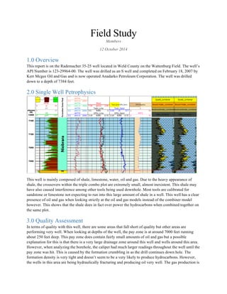
2.0 Single Well Petrophysics
This well is mainly composed of shale, limestone, water, oil and gas. Due to the heavy appearance of
shale, the crossovers within the triple combo plot are extremely small, almost inexistent. This shale may
have also caused interference among other tools being used downhole. Most tools are calibrated for
sandstone or limestone not expecting to run into this large amount of shale in a well. This well has a clear
presence of oil and gas when looking strictly at the oil and gas models instead of the combiner model
however. This shows that the shale does in fact over power the hydrocarbons when combined together on
the same plot.
3.0 Quality Assessment
In terms of quality with this well, there are some areas that fall short of quality but other areas are
performing very well. When looking at depths of the well, the pay zone is at around 7000 feet running
about 250 feet deep. This pay zone does contain fairly small amounts of oil and gas but a possible
explanation for this is that there is a very large drainage zone around this well and wells around this area.
However, when analyzing the borehole, the caliper had much larger readings throughout the well until the
pay zone was hit. This is caused by the formation crumbling in as the drill continues down hole. The
formation density is very tight and doesn’t seem to be a very likely to produce hydrocarbons. However,
the wells in this area are being hydraulically fracturing and producing oil very well. The gas production is

2. low because the hydraulic fracturing released the pressure allowing the gas cap to escape. The density of
the field remains consistent throughout all the down hole measurements therefore the density neutron
cross plot is accurate. The resistivity has also remained consistent throughout the hole making it’s reading
also accurate.
4.0 Analysis
Petrophysical analysis was done through multiple plots and charts to gain the values needed to
successfully analyze this well. Density neutron cross plots were made to find the density of the formation.
This density remained consistent throughout the hole and gave us a very accurate reading for our
formation density. A Pickett plot, along with a histogram, was used to find the Rw of the formation.
Multiple quanti elan plots were created for this formation. These plots were used to identify layers of
shale, oil, and gas. The plots made it clear that the target layer for this well was the Niobrara and Codell
because of the large gas and oil reserves that were shown. The gamma ray plot from the triple combo
layout was also used to interpret the fluids contained in the formation. All in all, this formation does
contain oil and gas and will produce hydrocarbons for whoever would like to pursue these plays.
4.1 Fluids

3. The initialization module was first run to calculate the resistivities of the flushed and the mud filtrate.
This module was also used to calculate values that would be used in future quanti elan modules.
Using the histogram, the lowest values were highlighted to show in the Pickett as the ones to use for the
Rw of the system.
I would estimate Rw to be about .045 based on the data editor and histogram above.
The Following Pickett Plot will prove this estimation at 0.04873ohm.m.
4.2 Lithology
Lithology was determined using a uma rhga cross plot and a Tnph_Lime Rhob cross plot. When these
were built, the lithologies were determined to be mainly composed of dolomite and calcite, which
comprise the limestone aspect of the formation.

4. 4.3 Porosity
Porosity was determined using a neutron density cross plot of the formation’s Rhob and Tnph_Lime.
Using these values shown in the cross plot, the porosities can be averaged over a certain period of depth.
4.4 Saturation
The saturation of the formation was found using archie’s equation.
Rw was found using the following histograms and cross plots and came out as 0.045 ohm.m.

5. Rt in the equation was found using the deep resistivity, AT90, and was averaged to be 24.5552 ohm.m.
We used AT90 as our formation resistivity because when looking at a log, the deepest resistivity gives the
most accurate reading for the formation resistivity.
Effective porosity was found using (Dphi_Lime+Tnph_Lime)/2 and was averaged to be 0.1204 g/cc.
Sw=((1/Phit^2)*(Rw/Rt))àSw=((1/0.1204^2)*(0.045/24.5552))àSw=35.55 %
Using the histogram, the lowest values were highlighted to show in the pickett as the ones to use for the
Rw of the system.

6. I would estimate Rw to be about .045 based on the data editor and histogram above.
The Following Pickett Plot will prove this estimation at 0.04873ohm.m.
5.0 Petrophysical Model
Four petrophysical models were created for shale, oil, gas and a combiner plot of the three. These plots
develop a representation of the components that comprise the model. The gas and oil models both showed
decent portions of the fluid until the combiner plot was made. When developing the combiner plot, it was
clear that the shale component was going to greatly outweigh the oil or gas component. When looking at
the triple combo plot, the shale layer showed much more prevalent than either fluid, thus proving the
assumption that shale will show more than the fluids in the combiner plot.
5.1 Assumptions
Our assumptions for the Dual Water Elan within our models were a=1, m=2 and n=2. The C value was 1
as well.
5.2 Model 1

7. Describe your model.
The model shown above is the shale model. As shown, the illite aspect of the plot shows up about half of
the time. The screenshot directly above shows the component specification for the plot. Calcite and
dolomite were included in all three quanti elan plots to account for the heavy amounts within the
formation. The gamma ray reading for the montmorillonite was increased to take some of the gamma ray
reading off of the shale to get a more accurate showing of the composition.
5.3 Model 2

8. The second model created was the quanti elan model for oil. This model showed a heavy presence of oil
in the pay zone at 7000 feet. The model still shows heavy amounts of illite, or shale, but does show the
presence of oil. The screenshot directly above shows the component specification for the model. Again,
calcite and dolomite were added to account for the heavy amounts within the formation from the lithology
cross plots above.
5.4 Model 3

9. The third quanti elan plot created was for the gas in the formation. As seen above, gas shows a heavy
presence throughout the formation but mainly in the pay zone, as it should. Again, illite plays a large role
in this plot but the gas is easily depicted. The screenshot above shows the component specifications for
the model where dolomite and calcite were added to account for the formation composition.
5.5 Combination Model

11. The fourth quanti elan plot was the combiner plot. The combiner plot takes the previous three plots and
combines them into one plot. The combiner plot showed exactly how the shale dominated this formation.
When looking at the previous three plots, you can see oil and gas clearly in the two that are designed for
that. However, when looking at the combiner plot, there are very few spots where oil can be noticed.
There are also no spots where gas can be seen. This proves that this well is shale dominant and a very
different well to interpret.
Describe your combination logic
6.0 Cased hole Analysis
6.1 Cement volume
Compute the cement volume required for your casing run
6.2 Bond Log
Evaluate the bond log
7.0 References
Colorado Oil and Gas Conservation Commission, cogcc.state.co.us
Tom Bratton’s Petrophysics Handbook