1. Using Scintillator Detection to Measure the Lifetime of Cosmic Ray Muons
Aaron Gruberg
(Dated: April 30, 2015)
The number of muon decay counts that occured inside a scintillator were measured. The number
of false decay counts was estimated and compared with the total decay count. These decay counts
were used to calculate the mean lifetime of a cosmic ray muon at rest to be τµ = 2.3170 ± 0.1231µ
seconds. This lifetime was a factor of 20 times smaller than the lifetime of a muon traveling at the
speed of light, which was evidence. The observed difference in lifetimes between muons at rest and
muons in motion was evidence for the relativistic effect of time dilation.
1. INTRODUCTION
Muon particles are produced by collisions between cos-
mic rays and the nuclei of air molecules in the top of
Earth’s atmosphere. These cosmic rays are approximated
to be 98% protons and heavier nuclei. The remaining 2%
are electrons. Of the protons and nuclei, about 87% are
protons, 12% are helium nuclei and the rest are heavier
nuclei that result from a process where nuclear fusion in
stars varies the chemical elements that are found in them.
This is called nucleosynthesis(Appendix A, Lifetime of
Cosmic Ray Muons). After the cosmic rays strike the
atmosphere a shower of secondary particles is produced
that includes protons, neutrons, pions, kaons, photons,
electrons, and positrons. These particles undergo elec-
tromagnetic and nuclear interactions which create more
particles. The pions from the secondary group can be
positevly, negatively, or neutrally charged. Some of the
charged pions interact with air molecules via the strong
force, others decay via the weak force, into a muon plus
a neutrino or antineutrino.
The muon only interacts with matter through the weak
and electromagnetic forces. It eventually decays into an
electron and a neutrino or antineutrino. The muon decay
distribution obeys a negative exponential curve.
N(t) = Noe−t/τµ
(1)
N(t) is the number of surviving muons at some time
t and No is the number of muons at t = 0. The decay
constant λ = 1/τµ, where τµ is the mean muon lifetime.
Inability to detect the neutrino and antineutrino is neg-
ligible. Muons travel at the speed of light and have a
mean production height of 15km, with a mean flight time
of 50µs. Muons lose their kinetic energy while traveling
from production height to sea level and a scintillator can
be used to measure their lifetime at rest. When cosmic
ray muons enter a scintillator and their kinetic energy
is transferred to the scintillator walls, electrons in the
scintillator material are excited to a higher energy state.
When they return to a lower energy state, a photon is
released. The emitted photon is the first pulse detected
by the scintillator. Once inside, some muons decay into
an electron plus a neutrino or antineutrino. The electron
produced in the decay of a muon is the second pulse.
The time interval between the first pulse from the muon
FIG. 1: Particles produced by cosmic ray proton striking an
air molecule nucleus.
entering the scintillator and the second pulse from the
muon decaying is the lifetime of the muon. The cosmic
ray flux at sea level integrated over all angles is one par-
ticle per square centimeter per minute, on any horizontal
surface. The flux through a vertical surface is half as
much. These statements can be used to make predic-
tions about the number of particles that pass through a
square centimeter of the scintillator every second. Given
the geometry of the detector, a 15cm diameter cylinder
with height 12.5cm, the predicted flux through the top of
the cylinder was 1particle/πr2
= 177 particles per square
centimeter per minute. The area of the side of the cylin-
der is 2πrh = 589cm2
. Because the flux through a ver-
tical surface is half a particle per square centimeter per
2. 2
minute, the predicted flux through the vertical area of the
cylinder was 295 particles per square centimeter and the
total predicted flux through the cylinder was predicted
to be 472 particles per square centimeter per minute or
8 particles per square centimeter per second. Not all of
these events would be muons traversing the scintillator
and as a result, this experiment needs to run for a suf-
ficient length of time to minimize the number of false
counts in the scintillator relative to muon decay counts.
If 8 muons pass through the cylinder every second, the
frequency by which false counts will occur is given by the
following expression.
Frequencyfalse = (
8muonsin
second
)(
8muonsout
second
)(8µseconds)
(2)
2. METHOD
A Teachspin Muon Physics apparatus was connected
via USB to a MS Windows-based computer.
FIG. 2: Muon Physics electronics box with a top view of scin-
tillator/photomultiplier tube cylinder. A tektronix TDS1002
digital oscilloscope was used to view pulses detected by the
photomultiplier tube(PMT).
The high voltage control of the scintillator determined
how sensitive the PMT was to radiated charges. The
high voltage control was turned to 70% in an attempt
to minimize the number of false counts while allowing a
high number of total counts. The discriminator thresh-
old control on the electronics box was turned 40% up.
This was used to filter out signals below a certain am-
plitude. If these low signals were not filtered out, elec-
trons produced inside the scintillator that did not arise
from incident photons would be more likely to trigger the
timer in the scintillator. This would increase the number
of false counts made. The PMT high voltage and dis-
criminator threshold voltage are coupled. The amplifier
output of the electronics box was connected to channel
one of the oscilloscope and the signals from the photo-
multiplier tube were directly observed. A 50Ω terminator
was installed on the end of the BNC cable connecting the
amplifier output to channel one. The discriminator out-
put of the electronics box was connected to channel two
of the oscilloscope.
FIG. 3: Oscilloscope display of a signal from the PMT on
channel one(bottom). Discriminator threshold voltage on
channel two.
Before data acquisition began, the output of the photo-
multiplier tube was observed directly on the oscilloscope.
A 350mV signal was displayed on channel 1 of the oscillo-
scope when a muon entered the scintillator. This signal
lasted about 75ns. As the high voltage control on the
scintillator increased, the PMT became more sensitive
and the time interval between succesive pulses became
smaller. As this control was decreased the PMT became
less sensitive. The Muon program was opened to begin
data acquisition. Once opened, ”Configure”, ”COM 3”
and ”Start” were selected. After a five minute run, the
muon decay histogram began to form. Each bin in the
histogram was one time interval that began when the
muon entered the cylinder and ended when the muon
decayed and an electron was produced. The height of
the the bin was the number of events in that time inter-
val. Each time interval should be a few µseconds long.
Events with longer time intervals likely resulted from
noise. The high voltage was measured to be 903V and
the discriminator threshold was 0.2V. Data aquisition be-
gan on 1/30/15 at 3:25pm and was stopped on 2/6/15 at
2:10pm. Data from the muon program was exported to
a .data file and imported into MatLab. A Matlab script
was written to filter out time intervals larger than 15000
nanoseconds. A plot of the number of counts vs. time
interval in nanoseconds was made. MatLab’s curve fit
tool named ”cftool” was used to fit a curve to the plot
3. 3
and obtain the exponential decay equation.
3. RESULTS
FIG. 4: Plot of the number of counts vs. time in nanosec-
onds. The number of counts at t = 0 was No = 444.λ =
0.0004455ns−1
, No = ±18, λ = ±0.000025ns−1
From the decay constant λ, the mean lifetime τµ was
calculated to be 2.24467 ± 0.1330µs. The number of de-
tector pulses per second that exceeded the discrimina-
tor threshold of the PMT was displayed on the Muon
Program with a value of 20 pulses per second. This
was more than twice the predicted value of 8 detector
pulses per second above threshold. The percentage un-
certainty in the number of counts at t = 0 was 4.1%.
The percentage uncertainty of the decay constant λ was
5.6%. The current accepted value for the mean lifetime
of a muon is τµ = 2.19703 ± 0.00004µseconds. The dis-
crepency between the calculated value and the accepted
value was 0.05µseconds, which was 2.1% of the accepted
value. There were time intervals greater than 15000ns
which had a large number of counts. The inclusion of
larger time intervals resulted in a poor exponential fit
and inaccurate calculation of the muon lifetime. For a
time interval of 20000ns the exponential probability dis-
tribution would be on the order of e−10
. This means the
probability of a muon having a lifetime of 20µs is very
small. Some counts in larger time intervals resulted from
systematic error in settings of the high voltage and dis-
criminator voltage control. They were excluded from 4.
A portion of the counts for time intervals greater than
15000ns resulted from electronic noise in the scintilla-
tor and contributed to random error in this experiment.
Possible causes for electronic noise were electrons pro-
duced in the scintillator that did not result from cosmic
rays and particles with a mass and energy close to that
of the muon. False counts were also produced by one
muon passing through the scintillator too closely behind
another. While a positively charged muon that stops in-
side the scintillator will decay, a negatively charged muon
that stops in the scintillator can bind to the carbon and
hydrogen nuclei in the scintillator walls, just as electrons
can. The Pauli exclusion principle does not prevent a
muon from occupying an orbital that is already filled
with electrons. The frequency of false counts was one
false count per 125 seconds as displayed by the muon
program. The total run time for this experiment was
601200 seconds. The total estimation of false counts is
601200/125 = 4810. This was 0.8% of the decay counts
and does not significantly effect the results of this exper-
iment.
4. CONCLUSION
The goal of this experiment was to measure the mean
lifetime of cosmic ray muons at rest. Time intervals be-
tween pairs of light pulses detected by a photomultiplier
tube in a scintillator were used to measure the number of
muon decays for a given time bin. The MatLab function
”cftool” was used to fit an exponential curve to the data
and calculate the decay constant which was used to calcu-
late the mean muon lifetime. This calculation of τµ was
within 2.1% of the accepted value. In future measure-
ments, the electronic noise could be decreased by setting
the discriminator voltage 5% higher so that fewer low am-
plitude signals are detected. Another way to acheive this
would be to make the detector less sensitive to pulses by
setting the high voltage 5% lower. Further exploration
can be done on other particles produced in the scintillator
that do not result from cosmic rays. The plot of number
of counts vs. time coulde be improved by downloading
the herrorbar package for horizontal error bars in Mat-
Lab plots. The first time interval recorded by the muon
program seemed to be produced by electronic noise. This
happened in multiple runs of the muon program. The fit
of the exponential curve to the distribution could be im-
proved by ignoring the first time bin. The muon lifetime
at rest is factor of 20 smaller than the muon lifetime trav-
eling near the speed of light. This appreciable difference
between the non-relativistic lifetime and the relativistic
lifetime was evidence for the time dilation effect of special
relativity.
[1] Dr. Roger Bland Lifetime of Cosmic Ray Muons.
[2] Dr. Bland’s script in MatLab