SlideShare a Scribd company logo
1 of 9
Download to read offline
SECTION 3.5

INVERSES OF MATRICES
The computational objective of this section is clearcut — to find the inverse of a given invertible
matrix. From a more general viewpoint, Theorem 7 on the properties of nonsingular matrices
summarizes most of the basic theory of this chapter.

In Problems 1-8 we first give the inverse matrix A −1 and then calculate the solution vector x.

                3 −2                    3 −2   5    3
1.      A −1 =       ;             x =         6  =  −2 
                −4 3                    −4 3         

                5 −7                    5 −7   −1    −26 
2.      A −1 =       ;             x =         3  =  11 
                −2 3                    −2 3             

                6 −7                    6 −7   2     33 
3.      A −1 =       ;             x =         −3 =  −28
                −5 6                    −5 6            

               17 −12                   17 −12  5    25 
4.      A −1 =        ;             x =         5 =  −10 
                −7 5                     −7 5            

                 1    4 −2                 1    4 −2   5  1  8 
5.      A −1 =        −5 3  ;       x =         −5 3  6  = 2  −7 
                 2                         2                  

                 1  6 −7                   1  6 −7  10  1  25 
        A −1 =                        x =                    =
                 3  −3 4                   3  −3 4   5  3  −10 
6.                          ;
                                                               

                 1    7 −9                 1    7 −9   3 1  3 
7.      A −1 =        −5 7  ;       x =         −5 7   2  = 4  −1
                 4                         4                   

                 1 10 −15                   1 10 −15 7  1  25 
        A −1 =                         x =                   =
                 5  −5 8                    5  −5 8   3 5  −11
8.                          ;
                                                              

In Problems 9-22 we give at least the first few steps in the reduction of the augmented matrix whose
right half is the identity matrix of appropriate size. We wind up with its echelon form, whose left
half is an identity matrix and whose right half is the desired inverse matrix.

        5 6 1 0          R1− R 2     1 1 1 −1          R 2− 4 R1   1 1 1 −1
9.      4 5 0 1           →         4 5 0 1              →         0 1 −4 5 
                                                                            
R1− R 2      1 0 5 −6                                5 −6 
          →           0 1 −4 5  ;               thus A −1 =       
                                                             −4 5 

      5 7 1 0           R1− R 2    1 1 1 −1               R 2− 4 R1   1 1 1 −1
10.   4 6 0 1            →         4 6 0 1                  →         0 2 −4 5 
                                                                               
        (1/ 2) R 2   1 1 1 −1                 R1− R 2   1 0 3 − 7                           1    6 −7 
          →          0 1 −2 5                  →        
                                                                     2
                                                                       ;       thus A −1 =          −4 5 
                            2                            0 1 −2 5 
                                                                   2                            2         

      1 5 1 1 0 0                 R 2− 2 R1
                                                  1 5 1 1 0 0 
11.   2 5 0 0 1 0                   →           0 −5 −2 −2 1 0 
                                                               
      2 7 1 0 0 1 
                                                2 7 1 0 0 1 
                                                                 

        R 3−2 R1
                      1 5 1 1 0 0                                   1 2 0 −1 0 1 
                                                            R1+ R3
           →          0 −5 −2 −2 1 0                       →        0 −5 −2 −2 1 0 
                                                                                     
                       0 −3 −1 − 2 0 1 
                                                                     0 −3 −1 − 2 0 1 
                                                                                       

        R 2− 2 R 3
                      1 2 0 −1 0 1                                      1 2 0 −1 0 1 
                                                              R 3+3 R 2
           →           0 1 0 2 1 −2                            →         0 1 0 2 1 −2 
                                                                                      
                      0 −3 −1 −2 0 1 
                                                                        0 0 −1 4 3 −5 
                                                                                        

        ( −1) R 3      R1−2 R 2
                                     1 0 0 −5 −2 5                                        − 5 −2 5 
          →             →           0 1 0 2 1 −2  ;                     thus A   −1
                                                                                         =  2 1 −2 
                                                                                                   
                                     0 0 1 −4 −3 5 
                                                                                          −4 −3 5 
                                                                                                     

      1 3 2 1 0 0                  R 2− 2 R1
                                                   1 3 2 1 0 0 
12.   2 8 3 0 1 0                    →           0 2 −1 −2 1 0 
                                                               
       3 10 6 0 0 1 
                                                  3 10 6 0 0 1 
                                                                 

        R 3−2 R1
                      1 3 2 1 0 0                                   1 3 2 1 0 0 
                                                          R 2− R 3
           →          0 2 −1 −2 1 0                       →         0 1 −1 1 1 −1
                                                                                  
                      0 1 0 −3 0 1 
                                                                     0 1 0 −3 0 1 
                                                                                    

                     1 3 2 1 0 0                         R1−3 R 2
                                                                          1 0 0 18 2 −7 
        R 3− R 2
          →          0 1 −1 1 1 −1                         →         → 0 1 0 −3 0 1  ;
                                                                                      
                     0 0 1 −4 −1 2 
                                                                        0 0 1 −4 −2 2 
                                                                                        

                       18 2 −7 
      thus A   −1
                     =  −3 0 1 
                                
                        −4 −1 2 
                                
2 7 3 1 0 0         SWAP ( R1, R 2)
                                              1 3 2 0 1 0 
13.   1 3 2 0 1 0              →            2 7 3 1 0 0
                                                        
      3 7 9 0 0 1 
                                            3 7 9 0 0 1 
                                                          

        R 2− 2 R1
                     1 3 2 0 1 0                          1 3 2 0 1 0 
                                               R 3−3 R1
          →           0 1 −1 1 −2 0            →           0 1 −1 1 −2 0 
                                                                         
                     3 7 9 0 0 1 
                                                          0 −2 3 0 −3 1 
                                                                           

                         1 0 0 −13 42 −5                                          −13 42 −5 
        R 3+ 2 R 2
          →           →  0 1 0 3 −9 1  ;
                                                              thus A      −1
                                                                                 =  3 −9 1 
                                                                                              
                         0 0 1 2 −7 1 
                                                                                  2 −7 1 
                                                                                              


      3 5 6 1 0 0                     1 1 3 1 −1 0 
                            R1− R 2
14.   2 4 3 0 1 0          →         2 4 3 0 1 0
                                                   
      2 3 5 0 0 1 
                                     2 3 5 0 0 1 
                                                     

                      1 1 3 1 −1 0                         1 1 3 1 −1 0 
        R 2− R 3                               R 3− 2 R1
          →           0 1 −2 0 1 −1            →          0 1 −2 0 1 −1
                                                                         
                     2 3 5 0 0 1 
                                                           0 1 −1 −2 2 1 
                                                                           

                         1 0 0 11 −7 −9                                       11 −7 −9 
        R 3− R 2
          →           →  0 1 0 −4 3 3  ;
                                                            thus A   −1
                                                                             =  −4 3 3 
                                                                                         
                          0 0 1 −2 1
                                     2                                       −2 1
                                                                                       2


      1 1 5 1 0 0                    1 1 5 1 0 0 
                             R 2− R1
15.   1 4 13 0 1 0          →         0 3 8 −1 1 0 
                                                   
      3 2 12 0 0 1 
                                     3 2 12 0 0 1 
                                                     

        R 3−3 R1
                     1 1 5 1 0 0                          1 1 5 1 0 0 
                                               R 2+ 2 R 3
          →           0 3 8 −1 1 0              →         0 1 2 −7 1 2 
                                                                         
                     0 −1 −3 −3 0 1 
                                                          0 −1 −3 −3 0 1 
                                                                           

                         1 0 0 −22 2 7                                            −22 2 7 
        R 3+ R 2
          →           → 0 1 0 −27 3 8  ;
                                                             thus A   −1
                                                                                 =  −27 3 8 
                                                                                            
                         0 0 1 10 −1 −3
                                                                                  10 −1 −3
                                                                                            
 1 −3 −3 1 0 0            R 2+ R1
                                             1 −3 −3 1 0 0 
16.    −1 1 2 0 1 0              →          0 −2 −1 1 1 0 
                                                          
       2 −3 −3 0 0 1 
                                            2 −3 −3 0 0 1 
                                                            

        R 3−2 R1
                       1 −3 −3 1 0 0                        1 −3 −3 1 0 0 
                                                R 2+ R 3
           →          0 −2 −1 1 1 0               →          0 1 2 −1 1 1 
                                                                          
                      0 3 3 −2 0 1 
                                                            0 3 3 −2 0 1 
                                                                            

        R 3−3 R 2
                       1 −3 − 3 1 0 0             ( −1/3( R 3)
                                                                    1 −3 − 3 1 0 0 
                      0 1 2 −1 1 1                                               
           →                                          →           0 1 2 −1 1 1 
                       0 0 −3 1 −3 −2 
                                                                 0 0 1 − 1 1 3 
                                                                              3
                                                                                  2
                                                                                    

        R1+3 R 2
                          1 0 0 −1 0 1                                         −3 0 3 
                                                                           =  −1 −3 −1
                                                                              1
          →           →  0 1 0 − 1 −1 − 1  ;
                                   3      3                    thus A   −1
                                                                                         
                                                                              3
                         0 0 1 − 1 1
                                  3
                                         2 
                                         3 
                                                                                 −1 3 2 
                                                                                        

       1 −3 0 1 0 0                         1 −3 0 1 0 0 
                                  R 2+ R1
                                 →          0 −1 −1 1 1 0 
17.    −1 2 −1 0 1 0                                      
       0 −2 2 0 0 1 
                                            0 −2 2 0 0 1 
                                                            

        ( −1) R 2
                      1 −3 0 1 0 0           R 3+ 2 R 2
                                                               1 −3 0 1 0 0
          →          0 1 1 −1 −1 0             →            0 1 1 −1 −1 0 
                                                                          
                     0 −2 2 0 0 1 
                                                            0 0 4 −2 −2 1 
                                                                            

        (1/ 4) R 3
                         1 0 0 − 1
                                  2            −2
                                                3
                                                      − 4
                                                        3
                                                                                      −2 −6 −3
                      → 0 1 0 − 1                   − 1;
                                                                                   1          
          →                      2            −1
                                                2       4         thus A    −1
                                                                                  =  −2 −2 −1
                                                                                   4
                         0 0 1 − 2
                         
                                  1
                                               −2
                                                1      1 
                                                       4 
                                                                                      −2 −2 1 
                                                                                              


      1 −2 2 1 0 0           R 2−3 R1
                                             1 −2 2 1 0 0 
                               →           0 6 −5 −3 1 0 
18.   3 0 1 0 1 0                                        
      1 −1 2 0 0 1 
                                           1 −1 2 0 0 1 
                                                           

                      1 −2 2 1 0 0           R 2−5 R 3
                                                               1 −2 2 1 0 0 
        R 3− R1
          →          0 6 −5 −3 1 0             →            0 1 −5 2 1 −5
                                                                          
                     0 1 0 −1 0 1 
                                                            0 1 0 −1 0 1 
                                                                            

                      1 −2 2 1 0 0                              1 0 0 1    2
                                                                                              − 5
                                                                                                2
        R 3− R 2                                                          5   5
                     0 1 −5 2 1 −5
                                                  (1/5) R 3
                                                                                              1 ;
          →                                       →          → 0 1 0 −1 0                     
                      0 0 5 −3 −1 6 
                                                                0 0 1 − 3 − 1
                                                                           5   5
                                                                                               6 
                                                                                               5 
 1 2 −2 
                    =  −5 0 5  .
               −1    1
      thus A                     
                     5
                        −3 −1 6 
                                


      1 4 3 1 0 0                        1 4 3 1 0 0
                                R 2− R1
19.   1 4 5 0 1 0              →          0 0 2 −1 1 0 
                                                       
      2 5 1 0 0 1 
                                         2 5 1 0 0 1 
                                                         

         SWAP ( R 2, R 3)
                            1 4 3 1 0 0            R 2− 2 R1
                                                                   1 4 3 1 0 0 
               →            2 5 1 0 0 1                  →       0 −3 −5 −2 0 1 
                                                                                
                             0 0 2 −1 1 0 
                                                                  0 0 2 −1 1 0 
                                                                                  

         ( −1/3) R 2
                       1 4 3 1 0 0                               1 0 0 − 72
                                                                                     11
                                                                                      6
                                                                                              4
                                                                                              3
                                                                                            − ;
                                                (1/ 2) R 3
            →          0 1 5 2 0 − 1             →            → 0 1 0 23
                                                                                 −      5         1
                            3  3    3                                                 6        3
                        0 0 2 −1 1 0 
                                                                 0 0 1 − 1
                                                                            2
                                                                                      1
                                                                                      2       0
                                                                                               

                        −21 11 8 
                    =  9 −5 −2 
               −1    1
      thus A                      
                     6
                        −3 3 0 
                                 


       2 0 −1 1 0 0                      1 0 −4 1 −1 0 
                                 R1− R 2
20.   1 0 3 0 1 0                →       1 0 3 0 1 0 
                                                       
      1 1 1 0 0 1 
                                         1 1 1 0 0 1 
                                                         

                     1 0 −4 1 −1 0                                1 0 −4 1 −1 0 
         R 3− R1                                SWAP ( R 2, R 3)
          →         1 0 3 0 1 0                     →             0 1 5 −1 1 1 
                                                                                
                    0 1 5 −1 1 0 
                                                                 1 0 3 0 1 0 
                                                                                  

                     1 0 −4 1 − 1 0                            1 0 0 73       1
                                                                                            0
         R 3− R1                                                                 7
                                    
                                               (1/7) R 3
                                                                                            
          →         0 1 5 −1 1 1               →            → 0 1 0 − 72
                                                                                 −   3
                                                                                     7      1 ;
                    0 0 7 −1 2 0 
                                                               0 0 1 − 1
                                                                          7
                                                                                 2
                                                                                 7          0
                                                                                             

                        3 1 0
                    =  −2 −3 7 
                     1
      thus A −1                 
                     7
                        −1 2 0 
                               
0    0    1      0     1    0       0       0                              1    0     0    0    0       1       0       0
        1    0    0      0     0    1       0       0          SWAP ( R1, R 2)     0    0     1    0    1       0       0       0
21.                                                                  →                                                           
        0    1    2      0     0    0       1       0                              0    1     2    0    0       0       1       0
                                                                                                                                 
        3    0    0      1     0    0       0       1                              3    0     0    1    0       0       0       1

                                    1       0       0       0     0    1      0     0               1       0       0       0    0 1      0   0
             SWAP ( R 2, R 3)       0       1       2       0     0    0      1     0   R 4 −3 R1   0       1       2       0    0 0      1   0
                   →                                                                        →                                                  
                                    0       0       1       0     1    0      0     0               0       0       1       0    1 0      0   0
                                                                                                                                               
                                    3       0       0       1     0    0      0     1               0       0       0       1    0 −3     0   1

                          1    0        0       0 0 1                     0    0                           0 1                   0   0
             R 2− 2 R 3   0    1        0       0 −2 0                    1    0                            −2 0                 1   0
               →                                                                ;       thus A −1        =                            
                          0    0        1       0 1 0                     0    0                           1 0                   0   0
                                                                                                                                      
                          0    0        0       1 0 −3                    0    1                            0 −3                 0   1


        4    0     1     1     1    0       0       0                        1 −1 −2           0   1 −1             0       0
        3    1     3     1     0    1       0       0          R1− R 2       3 1 3             1   0 1              0       0
22.                                                             →                                                            
        0    1     2     0     0    0       1       0                        0 1 2             0   0 0              1       0
                                                                                                                             
        3    2     4     1     0    0       0       1                        3 2 4             1   0 0              0       1

                    1 −1 −2                 0 1 −1                        0    0                1 −1 −2                 0 1 −1            0   0
        R 2−3 R1    0 4 9                   1 −3 4                        0    0    R 4−3 R1    0 4 9                   1 −3 4            0   0
          →                                                                             →                                                      
                    0 1 2                   0 0 0                         1    0                0 1 2                   0 0 0             1   0
                                                                                                                                               
                    3 2 4                   1 0 0                         0    1                 0 5 10                 1 −3 3            0   1

                   1 −1 −2                  0 1 −1 0                           0               1 −1 −2 0 1 −1 0                                0
        R 2−3 R3   0 1 3                    1 −3 4 −3                          0    R3− R 2    0 1 3 1 −3 4 −3                                 0
          →                                                                             →                                                       
                   0 1 2                    0 0 0 1                            0               0 0 −1 −1 3 −4 4                                0
                                                                                                                                                
                   0 5 10                   1 −3 3 0                           1               0 5 10 1 −3 3 0                                 1

                              1                 0       0       0 1 −1 1 0               1 −1 1 0 
             R 4−5 R 2        0                 1       0                   
                                                                 0 0 −2 −1 2              0 −2 −1 2 
               →           →                                                 ; thus A = 
                                                                                       −1             
                              0                 0       1       0 0 1 1 −1               0 1 1 −1
                                                                                                   
                              0                 0       0       1 −3 3 −5 1              −3 3 −5 1 

In Problems 23-28 we first give the inverse matrix A −1 and then calculate the solution matrix X.

                4 −3                            4 −3  1 3 −5       7 18 −35
23.     A −1 =       ;                     X =         −1 −2 5  =  −9 −23 45 
                −5 4                            −5 4                         
 7 −6                     7 −6   2 0 4    14 −30 46 
24.   A −1 =       ;              X =        0 5 −3 =  −16 35 −53
              −8 7                     −8 7                      

                  11 −9 4                    11 −9 4   1 0 3    7 −14 15 
25.   A   −1
               =  −2 2 −1 ;
                          
                                               −2 2 −1  0 2 2  =  −1 3 −2 
                                          X =                              
                  −2 1 0 
                                             −2 1 0   −1 1 0 
                                                                  −2 2 −4 
                                                                               

                  −16 3 11                     −16 3 11   2 0 1    −21 9 6 
26.   A   −1
               =  6 −1 −4  ;
                           
                                                 6 −1 −4   0 3 0  =  8 −3 −2
                                            X =                              
                  −13 2 9 
                                               −13 2 9  1 0 2 
                                                                     −17 6 5 
                                                                                 

                  7 −20 17        7 −20 17  0 0 1 1    17 −20 24 −13
27.   A   −1     0
               =     −1 1 ; X =  0         0 1 0 1  =  1
                                        −1 1                    −1 1   −1 
                                                                         
                  −2 6 −5 
                                  −2 6 −5   1 0 1 0 
                                                          −5 6 −7 4 
                                                                           

          −5 5   10         −5 5   10   2 1 0 2   −5 5    10  1 
28.       −8 8
      A =−1          ; X =  −8 8
                  15                      −1 3 5 0  =  −8 8
                                      15                       15  7 
                                                                    
          24 −23 −45
                            24 −23 −45  1 1 0 5   24 −23 −45 −13
                                                                  

29.   (a)    The fact that A–1 is the inverse of A means that AA −1 = A −1A = I. That is, that
      when A–1 is multiplied either on the right or on the left by A, the result is the identity
      matrix I. By the same token, this means that A is the inverse of A–1.
      (b)        A n ( A −1 ) n = A n −1 ⋅ AA −1 ⋅ ( A −1 ) n −1 = A n −1 ⋅ I ⋅ ( A −1 ) n −1 =  = I. Similarly,
      ( A −1 )n A n = I , so it follows that ( A −1 ) n is the inverse of A n .

30.   ABC ⋅ C−1B −1A −1 = AB ⋅ I ⋅ B −1A −1 = A ⋅ I ⋅ A −1 = I, and we see is a similar way that
      C−1B −1A −1 ⋅ ABC = I.

31.   Let p = − r  0, q = − s  0, and B = A −1. Then

                           A r A s = A − p A − q = ( A −1 ) p ( A −1 ) q
                                   = B pBq = B p+q             (because p, q  0)
                                   = ( A −1 ) p + q = A − p − q = A r + s

      as desired, and ( A r )s = ( A − p ) − q = (B p ) − q = B − pq = A pq = A rs similarly.

32.   Multiplication of AB = AC on the left by A–1 yields B = C.
33.   In particular, Ae j = e j where e j denotes the jth column vector of the identity matrix I.
      Hence it follows from Fact 2 that AI = I, and therefore A = I–1 = I.

34.   The invertibility of a diagonal matrix with nonzero diagonal elements follows immediately
      from the rule for multiplying diagonal matrices (Problem 27 in Section 3.4). The inverse of
      such a diagonal matrix is gotten simply by inverting each diagonal element.

35.   If the jth column of A is all zeros and B is any n × n matrix, then the jth column of BA is
      all zeros, so BA ≠ I. Hence A has no inverse matrix. Similarly, if the ith row of A is all
      zeros, then so is the ith row of AB.

36.   If ad – bc = 0, then it follows easily that one row of A is a multiple of the other. Hence the
                                                    * * 
      reduced echelon form of A is of the form            rather than the 2 × 2 identity matrix.
                                                    0 0 
      Therefore A is not invertible.

37.   Direct multiplication shows that AA −1 = A −1A = I.

           3 0   a b   3a 3b 
38.   EA =      c d  =  c d 
           0 1               

           1 0 0   a11       a12   a13     a11              a12         a13 
39.   EA = 0 1 0   a21
                             a22        =  a
                                      a23          21          a22         a23   
            2 0 1   a31
                             a32   a33 
                                              a31 + 2a11
                                                             a32 + a12   a33 + a13 
                                                                                    

           0 1 0   a11       a12   a13     a21   a22    a23 
40.   EA = 1 0 0   a21
                             a22        = a
                                      a23     11    a12    a13 
                                                                 
           0 0 1   a31
                             a32   a33 
                                              a31
                                                     a32    a33 
                                                                 

41.   This follows immediately from the fact that the ijth element of AB is the product of the ith
      row of A and the jth column of B.

42.   Let ei denote the ith row of I. Then ei B = B i , the ith row of B. Hence the result in
      Problem 41 yields

                            e1    e1B      B1 
                           e     e B      B 
                      IB =   B = 
                                      2 
                              2
                                            =  2  = B.
                                          
                                           
                           e m 
                                 e m B 
                                            B m 
                                               
43.   Let E1 , E2 ,  , Ek be the elementary matrices corresponding to the elementary row
      operations that reduce A to B. Then Theorem 5 gives B = Ek Ek −1  E2 E1A = GA where
      G = E k E k −1  E2 E1.

44.   This follows immediately from the result in Problem 43, because an invertible matrix is
      row-equivalent to the identity matrix.

45.   One can simply photocopy the portion of the proof of Theorem 7 that follows Equation (20).
      Starting only with the assumption that A and B are square matrices with AB = I, it is
      proved there that A and B are then invertible.

46.   If C = AB is invertible, so C–1 exists, then A(BC−1 ) = I and (C−1 A)B = I. Hence the
      fact that A and B are invertible follows immediately from Problem 45.

More Related Content

Similar to Sect3 5

Determinants, Properties and IMT
Determinants, Properties and IMTDeterminants, Properties and IMT
Determinants, Properties and IMTPrasanth George
 
Tutorial 8 mth 3201
Tutorial 8 mth 3201Tutorial 8 mth 3201
Tutorial 8 mth 3201Drradz Maths
 
Systems of Linear Equations, RREF
Systems of Linear Equations, RREFSystems of Linear Equations, RREF
Systems of Linear Equations, RREFPrasanth George
 
solucionario de purcell 0
solucionario de purcell 0solucionario de purcell 0
solucionario de purcell 0José Encalada
 
001 matrices and_determinants
001 matrices and_determinants001 matrices and_determinants
001 matrices and_determinantsphysics101
 
Molecular mapping of an ATP insensitive Arabidopsis thaliana mutant
Molecular mapping of an ATP insensitive Arabidopsis thaliana mutantMolecular mapping of an ATP insensitive Arabidopsis thaliana mutant
Molecular mapping of an ATP insensitive Arabidopsis thaliana mutantBlake Stephens
 
College Algebra Chapters 1 and 2
College Algebra Chapters 1 and 2College Algebra Chapters 1 and 2
College Algebra Chapters 1 and 2jeanperryshields
 
Graph functions
Graph functionsGraph functions
Graph functionsdaisy_yani
 
Tutorial 5 mth 3201
Tutorial 5 mth 3201Tutorial 5 mth 3201
Tutorial 5 mth 3201Drradz Maths
 
Conics foldable
Conics foldableConics foldable
Conics foldabletdpturner
 
Lesson 18: Geometric Representations of Functions
Lesson 18: Geometric Representations of FunctionsLesson 18: Geometric Representations of Functions
Lesson 18: Geometric Representations of FunctionsMatthew Leingang
 
Sheda esercizi n1 calcolo del dominio
Sheda esercizi n1   calcolo del dominioSheda esercizi n1   calcolo del dominio
Sheda esercizi n1 calcolo del dominioESmargiassi
 

Similar to Sect3 5 (20)

Sect3 3
Sect3 3Sect3 3
Sect3 3
 
0909 ch 9 day 9
0909 ch 9 day 90909 ch 9 day 9
0909 ch 9 day 9
 
Determinants, Properties and IMT
Determinants, Properties and IMTDeterminants, Properties and IMT
Determinants, Properties and IMT
 
Tutorial 8 mth 3201
Tutorial 8 mth 3201Tutorial 8 mth 3201
Tutorial 8 mth 3201
 
Matrix opt
Matrix optMatrix opt
Matrix opt
 
Systems of Linear Equations, RREF
Systems of Linear Equations, RREFSystems of Linear Equations, RREF
Systems of Linear Equations, RREF
 
Sol00
Sol00Sol00
Sol00
 
solucionario de purcell 0
solucionario de purcell 0solucionario de purcell 0
solucionario de purcell 0
 
001 matrices and_determinants
001 matrices and_determinants001 matrices and_determinants
001 matrices and_determinants
 
Echelon or not
Echelon or notEchelon or not
Echelon or not
 
Molecular mapping of an ATP insensitive Arabidopsis thaliana mutant
Molecular mapping of an ATP insensitive Arabidopsis thaliana mutantMolecular mapping of an ATP insensitive Arabidopsis thaliana mutant
Molecular mapping of an ATP insensitive Arabidopsis thaliana mutant
 
College Algebra Chapters 1 and 2
College Algebra Chapters 1 and 2College Algebra Chapters 1 and 2
College Algebra Chapters 1 and 2
 
Math11
Math11Math11
Math11
 
Graph functions
Graph functionsGraph functions
Graph functions
 
Matrix Inverse, IMT
Matrix Inverse, IMTMatrix Inverse, IMT
Matrix Inverse, IMT
 
Tutorial 5 mth 3201
Tutorial 5 mth 3201Tutorial 5 mth 3201
Tutorial 5 mth 3201
 
Maximum and minimum
Maximum and minimumMaximum and minimum
Maximum and minimum
 
Conics foldable
Conics foldableConics foldable
Conics foldable
 
Lesson 18: Geometric Representations of Functions
Lesson 18: Geometric Representations of FunctionsLesson 18: Geometric Representations of Functions
Lesson 18: Geometric Representations of Functions
 
Sheda esercizi n1 calcolo del dominio
Sheda esercizi n1   calcolo del dominioSheda esercizi n1   calcolo del dominio
Sheda esercizi n1 calcolo del dominio
 

More from inKFUPM (20)

Tb10
Tb10Tb10
Tb10
 
Tb18
Tb18Tb18
Tb18
 
Tb14
Tb14Tb14
Tb14
 
Tb13
Tb13Tb13
Tb13
 
Tb17
Tb17Tb17
Tb17
 
Tb16
Tb16Tb16
Tb16
 
Tb15
Tb15Tb15
Tb15
 
Tb12
Tb12Tb12
Tb12
 
Tb11
Tb11Tb11
Tb11
 
Tb09
Tb09Tb09
Tb09
 
Tb05
Tb05Tb05
Tb05
 
Tb07
Tb07Tb07
Tb07
 
Tb04
Tb04Tb04
Tb04
 
Tb02
Tb02Tb02
Tb02
 
Tb03
Tb03Tb03
Tb03
 
Tb06
Tb06Tb06
Tb06
 
Tb01
Tb01Tb01
Tb01
 
Tb08
Tb08Tb08
Tb08
 
21221
2122121221
21221
 
Sect5 6
Sect5 6Sect5 6
Sect5 6
 

Recently uploaded

Scaling API-first – The story of a global engineering organization
Scaling API-first – The story of a global engineering organizationScaling API-first – The story of a global engineering organization
Scaling API-first – The story of a global engineering organizationRadu Cotescu
 
Bajaj Allianz Life Insurance Company - Insurer Innovation Award 2024
Bajaj Allianz Life Insurance Company - Insurer Innovation Award 2024Bajaj Allianz Life Insurance Company - Insurer Innovation Award 2024
Bajaj Allianz Life Insurance Company - Insurer Innovation Award 2024The Digital Insurer
 
TrustArc Webinar - Unlock the Power of AI-Driven Data Discovery
TrustArc Webinar - Unlock the Power of AI-Driven Data DiscoveryTrustArc Webinar - Unlock the Power of AI-Driven Data Discovery
TrustArc Webinar - Unlock the Power of AI-Driven Data DiscoveryTrustArc
 
Strategies for Landing an Oracle DBA Job as a Fresher
Strategies for Landing an Oracle DBA Job as a FresherStrategies for Landing an Oracle DBA Job as a Fresher
Strategies for Landing an Oracle DBA Job as a FresherRemote DBA Services
 
Apidays Singapore 2024 - Building Digital Trust in a Digital Economy by Veron...
Apidays Singapore 2024 - Building Digital Trust in a Digital Economy by Veron...Apidays Singapore 2024 - Building Digital Trust in a Digital Economy by Veron...
Apidays Singapore 2024 - Building Digital Trust in a Digital Economy by Veron...apidays
 
Automating Google Workspace (GWS) & more with Apps Script
Automating Google Workspace (GWS) & more with Apps ScriptAutomating Google Workspace (GWS) & more with Apps Script
Automating Google Workspace (GWS) & more with Apps Scriptwesley chun
 
Understanding Discord NSFW Servers A Guide for Responsible Users.pdf
Understanding Discord NSFW Servers A Guide for Responsible Users.pdfUnderstanding Discord NSFW Servers A Guide for Responsible Users.pdf
Understanding Discord NSFW Servers A Guide for Responsible Users.pdfUK Journal
 
Apidays New York 2024 - The value of a flexible API Management solution for O...
Apidays New York 2024 - The value of a flexible API Management solution for O...Apidays New York 2024 - The value of a flexible API Management solution for O...
Apidays New York 2024 - The value of a flexible API Management solution for O...apidays
 
Boost Fertility New Invention Ups Success Rates.pdf
Boost Fertility New Invention Ups Success Rates.pdfBoost Fertility New Invention Ups Success Rates.pdf
Boost Fertility New Invention Ups Success Rates.pdfsudhanshuwaghmare1
 
From Event to Action: Accelerate Your Decision Making with Real-Time Automation
From Event to Action: Accelerate Your Decision Making with Real-Time AutomationFrom Event to Action: Accelerate Your Decision Making with Real-Time Automation
From Event to Action: Accelerate Your Decision Making with Real-Time AutomationSafe Software
 
Artificial Intelligence Chap.5 : Uncertainty
Artificial Intelligence Chap.5 : UncertaintyArtificial Intelligence Chap.5 : Uncertainty
Artificial Intelligence Chap.5 : UncertaintyKhushali Kathiriya
 
The 7 Things I Know About Cyber Security After 25 Years | April 2024
The 7 Things I Know About Cyber Security After 25 Years | April 2024The 7 Things I Know About Cyber Security After 25 Years | April 2024
The 7 Things I Know About Cyber Security After 25 Years | April 2024Rafal Los
 
Workshop - Best of Both Worlds_ Combine KG and Vector search for enhanced R...
Workshop - Best of Both Worlds_ Combine  KG and Vector search for  enhanced R...Workshop - Best of Both Worlds_ Combine  KG and Vector search for  enhanced R...
Workshop - Best of Both Worlds_ Combine KG and Vector search for enhanced R...Neo4j
 
Deploy with confidence: VMware Cloud Foundation 5.1 on next gen Dell PowerEdg...
Deploy with confidence: VMware Cloud Foundation 5.1 on next gen Dell PowerEdg...Deploy with confidence: VMware Cloud Foundation 5.1 on next gen Dell PowerEdg...
Deploy with confidence: VMware Cloud Foundation 5.1 on next gen Dell PowerEdg...Principled Technologies
 
Data Cloud, More than a CDP by Matt Robison
Data Cloud, More than a CDP by Matt RobisonData Cloud, More than a CDP by Matt Robison
Data Cloud, More than a CDP by Matt RobisonAnna Loughnan Colquhoun
 
A Domino Admins Adventures (Engage 2024)
A Domino Admins Adventures (Engage 2024)A Domino Admins Adventures (Engage 2024)
A Domino Admins Adventures (Engage 2024)Gabriella Davis
 
Strategize a Smooth Tenant-to-tenant Migration and Copilot Takeoff
Strategize a Smooth Tenant-to-tenant Migration and Copilot TakeoffStrategize a Smooth Tenant-to-tenant Migration and Copilot Takeoff
Strategize a Smooth Tenant-to-tenant Migration and Copilot Takeoffsammart93
 
Tata AIG General Insurance Company - Insurer Innovation Award 2024
Tata AIG General Insurance Company - Insurer Innovation Award 2024Tata AIG General Insurance Company - Insurer Innovation Award 2024
Tata AIG General Insurance Company - Insurer Innovation Award 2024The Digital Insurer
 
How to Troubleshoot Apps for the Modern Connected Worker
How to Troubleshoot Apps for the Modern Connected WorkerHow to Troubleshoot Apps for the Modern Connected Worker
How to Troubleshoot Apps for the Modern Connected WorkerThousandEyes
 
Artificial Intelligence: Facts and Myths
Artificial Intelligence: Facts and MythsArtificial Intelligence: Facts and Myths
Artificial Intelligence: Facts and MythsJoaquim Jorge
 

Recently uploaded (20)

Scaling API-first – The story of a global engineering organization
Scaling API-first – The story of a global engineering organizationScaling API-first – The story of a global engineering organization
Scaling API-first – The story of a global engineering organization
 
Bajaj Allianz Life Insurance Company - Insurer Innovation Award 2024
Bajaj Allianz Life Insurance Company - Insurer Innovation Award 2024Bajaj Allianz Life Insurance Company - Insurer Innovation Award 2024
Bajaj Allianz Life Insurance Company - Insurer Innovation Award 2024
 
TrustArc Webinar - Unlock the Power of AI-Driven Data Discovery
TrustArc Webinar - Unlock the Power of AI-Driven Data DiscoveryTrustArc Webinar - Unlock the Power of AI-Driven Data Discovery
TrustArc Webinar - Unlock the Power of AI-Driven Data Discovery
 
Strategies for Landing an Oracle DBA Job as a Fresher
Strategies for Landing an Oracle DBA Job as a FresherStrategies for Landing an Oracle DBA Job as a Fresher
Strategies for Landing an Oracle DBA Job as a Fresher
 
Apidays Singapore 2024 - Building Digital Trust in a Digital Economy by Veron...
Apidays Singapore 2024 - Building Digital Trust in a Digital Economy by Veron...Apidays Singapore 2024 - Building Digital Trust in a Digital Economy by Veron...
Apidays Singapore 2024 - Building Digital Trust in a Digital Economy by Veron...
 
Automating Google Workspace (GWS) & more with Apps Script
Automating Google Workspace (GWS) & more with Apps ScriptAutomating Google Workspace (GWS) & more with Apps Script
Automating Google Workspace (GWS) & more with Apps Script
 
Understanding Discord NSFW Servers A Guide for Responsible Users.pdf
Understanding Discord NSFW Servers A Guide for Responsible Users.pdfUnderstanding Discord NSFW Servers A Guide for Responsible Users.pdf
Understanding Discord NSFW Servers A Guide for Responsible Users.pdf
 
Apidays New York 2024 - The value of a flexible API Management solution for O...
Apidays New York 2024 - The value of a flexible API Management solution for O...Apidays New York 2024 - The value of a flexible API Management solution for O...
Apidays New York 2024 - The value of a flexible API Management solution for O...
 
Boost Fertility New Invention Ups Success Rates.pdf
Boost Fertility New Invention Ups Success Rates.pdfBoost Fertility New Invention Ups Success Rates.pdf
Boost Fertility New Invention Ups Success Rates.pdf
 
From Event to Action: Accelerate Your Decision Making with Real-Time Automation
From Event to Action: Accelerate Your Decision Making with Real-Time AutomationFrom Event to Action: Accelerate Your Decision Making with Real-Time Automation
From Event to Action: Accelerate Your Decision Making with Real-Time Automation
 
Artificial Intelligence Chap.5 : Uncertainty
Artificial Intelligence Chap.5 : UncertaintyArtificial Intelligence Chap.5 : Uncertainty
Artificial Intelligence Chap.5 : Uncertainty
 
The 7 Things I Know About Cyber Security After 25 Years | April 2024
The 7 Things I Know About Cyber Security After 25 Years | April 2024The 7 Things I Know About Cyber Security After 25 Years | April 2024
The 7 Things I Know About Cyber Security After 25 Years | April 2024
 
Workshop - Best of Both Worlds_ Combine KG and Vector search for enhanced R...
Workshop - Best of Both Worlds_ Combine  KG and Vector search for  enhanced R...Workshop - Best of Both Worlds_ Combine  KG and Vector search for  enhanced R...
Workshop - Best of Both Worlds_ Combine KG and Vector search for enhanced R...
 
Deploy with confidence: VMware Cloud Foundation 5.1 on next gen Dell PowerEdg...
Deploy with confidence: VMware Cloud Foundation 5.1 on next gen Dell PowerEdg...Deploy with confidence: VMware Cloud Foundation 5.1 on next gen Dell PowerEdg...
Deploy with confidence: VMware Cloud Foundation 5.1 on next gen Dell PowerEdg...
 
Data Cloud, More than a CDP by Matt Robison
Data Cloud, More than a CDP by Matt RobisonData Cloud, More than a CDP by Matt Robison
Data Cloud, More than a CDP by Matt Robison
 
A Domino Admins Adventures (Engage 2024)
A Domino Admins Adventures (Engage 2024)A Domino Admins Adventures (Engage 2024)
A Domino Admins Adventures (Engage 2024)
 
Strategize a Smooth Tenant-to-tenant Migration and Copilot Takeoff
Strategize a Smooth Tenant-to-tenant Migration and Copilot TakeoffStrategize a Smooth Tenant-to-tenant Migration and Copilot Takeoff
Strategize a Smooth Tenant-to-tenant Migration and Copilot Takeoff
 
Tata AIG General Insurance Company - Insurer Innovation Award 2024
Tata AIG General Insurance Company - Insurer Innovation Award 2024Tata AIG General Insurance Company - Insurer Innovation Award 2024
Tata AIG General Insurance Company - Insurer Innovation Award 2024
 
How to Troubleshoot Apps for the Modern Connected Worker
How to Troubleshoot Apps for the Modern Connected WorkerHow to Troubleshoot Apps for the Modern Connected Worker
How to Troubleshoot Apps for the Modern Connected Worker
 
Artificial Intelligence: Facts and Myths
Artificial Intelligence: Facts and MythsArtificial Intelligence: Facts and Myths
Artificial Intelligence: Facts and Myths
 

Sect3 5

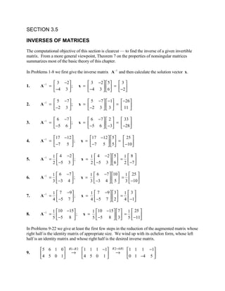
  • 1. SECTION 3.5 INVERSES OF MATRICES The computational objective of this section is clearcut — to find the inverse of a given invertible matrix. From a more general viewpoint, Theorem 7 on the properties of nonsingular matrices summarizes most of the basic theory of this chapter. In Problems 1-8 we first give the inverse matrix A −1 and then calculate the solution vector x.  3 −2   3 −2   5  3 1. A −1 =  ; x =    6  =  −2   −4 3   −4 3       5 −7   5 −7   −1  −26  2. A −1 =  ; x =    3  =  11   −2 3   −2 3       6 −7   6 −7   2   33  3. A −1 =  ; x =    −3 =  −28  −5 6   −5 6      17 −12  17 −12  5  25  4. A −1 =  ; x =   5 =  −10   −7 5   −7 5      1  4 −2  1  4 −2   5  1  8  5. A −1 =  −5 3  ; x =  −5 3  6  = 2  −7  2   2      1  6 −7  1  6 −7  10  1  25  A −1 = x = = 3  −3 4  3  −3 4   5  3  −10  6. ;        1  7 −9  1  7 −9   3 1  3  7. A −1 =  −5 7  ; x =  −5 7   2  = 4  −1 4   4      1 10 −15 1 10 −15 7  1  25  A −1 = x = = 5  −5 8  5  −5 8   3 5  −11 8. ;        In Problems 9-22 we give at least the first few steps in the reduction of the augmented matrix whose right half is the identity matrix of appropriate size. We wind up with its echelon form, whose left half is an identity matrix and whose right half is the desired inverse matrix. 5 6 1 0 R1− R 2  1 1 1 −1 R 2− 4 R1 1 1 1 −1 9. 4 5 0 1  → 4 5 0 1  → 0 1 −4 5       
  • 2. R1− R 2 1 0 5 −6   5 −6  →  0 1 −4 5  ; thus A −1 =      −4 5  5 7 1 0 R1− R 2 1 1 1 −1 R 2− 4 R1 1 1 1 −1 10. 4 6 0 1  → 4 6 0 1  → 0 2 −4 5        (1/ 2) R 2 1 1 1 −1 R1− R 2 1 0 3 − 7  1  6 −7  → 0 1 −2 5  →  2 ; thus A −1 =  −4 5   2   0 1 −2 5  2 2   1 5 1 1 0 0  R 2− 2 R1 1 5 1 1 0 0  11. 2 5 0 0 1 0 → 0 −5 −2 −2 1 0      2 7 1 0 0 1    2 7 1 0 0 1    R 3−2 R1 1 5 1 1 0 0  1 2 0 −1 0 1  R1+ R3 → 0 −5 −2 −2 1 0  → 0 −5 −2 −2 1 0       0 −3 −1 − 2 0 1     0 −3 −1 − 2 0 1    R 2− 2 R 3 1 2 0 −1 0 1  1 2 0 −1 0 1  R 3+3 R 2 →  0 1 0 2 1 −2  →  0 1 0 2 1 −2      0 −3 −1 −2 0 1    0 0 −1 4 3 −5    ( −1) R 3 R1−2 R 2  1 0 0 −5 −2 5   − 5 −2 5  → →  0 1 0 2 1 −2  ; thus A −1 =  2 1 −2       0 0 1 −4 −3 5     −4 −3 5    1 3 2 1 0 0  R 2− 2 R1 1 3 2 1 0 0  12. 2 8 3 0 1 0  → 0 2 −1 −2 1 0       3 10 6 0 0 1     3 10 6 0 0 1    R 3−2 R1 1 3 2 1 0 0  1 3 2 1 0 0  R 2− R 3 → 0 2 −1 −2 1 0  → 0 1 −1 1 1 −1     0 1 0 −3 0 1     0 1 0 −3 0 1    1 3 2 1 0 0  R1−3 R 2 1 0 0 18 2 −7  R 3− R 2 → 0 1 −1 1 1 −1 → → 0 1 0 −3 0 1  ;     0 0 1 −4 −1 2    0 0 1 −4 −2 2    18 2 −7  thus A −1 =  −3 0 1     −4 −1 2   
  • 3. 2 7 3 1 0 0 SWAP ( R1, R 2) 1 3 2 0 1 0  13. 1 3 2 0 1 0 → 2 7 3 1 0 0     3 7 9 0 0 1    3 7 9 0 0 1    R 2− 2 R1 1 3 2 0 1 0  1 3 2 0 1 0  R 3−3 R1 →  0 1 −1 1 −2 0  →  0 1 −1 1 −2 0      3 7 9 0 0 1    0 −2 3 0 −3 1    1 0 0 −13 42 −5  −13 42 −5  R 3+ 2 R 2 → →  0 1 0 3 −9 1  ;   thus A −1 =  3 −9 1    0 0 1 2 −7 1     2 −7 1    3 5 6 1 0 0   1 1 3 1 −1 0  R1− R 2 14. 2 4 3 0 1 0  → 2 4 3 0 1 0     2 3 5 0 0 1    2 3 5 0 0 1     1 1 3 1 −1 0   1 1 3 1 −1 0  R 2− R 3 R 3− 2 R1 →  0 1 −2 0 1 −1 → 0 1 −2 0 1 −1     2 3 5 0 0 1     0 1 −1 −2 2 1    1 0 0 11 −7 −9   11 −7 −9  R 3− R 2 → →  0 1 0 −4 3 3  ;   thus A −1 =  −4 3 3     0 0 1 −2 1  2   −2 1  2 1 1 5 1 0 0  1 1 5 1 0 0  R 2− R1 15. 1 4 13 0 1 0  →  0 3 8 −1 1 0      3 2 12 0 0 1    3 2 12 0 0 1    R 3−3 R1 1 1 5 1 0 0  1 1 5 1 0 0  R 2+ 2 R 3 →  0 3 8 −1 1 0  → 0 1 2 −7 1 2      0 −1 −3 −3 0 1    0 −1 −3 −3 0 1    1 0 0 −22 2 7   −22 2 7  R 3+ R 2 → → 0 1 0 −27 3 8  ;   thus A −1 =  −27 3 8    0 0 1 10 −1 −3    10 −1 −3  
  • 4.  1 −3 −3 1 0 0  R 2+ R1 1 −3 −3 1 0 0  16.  −1 1 2 0 1 0  →  0 −2 −1 1 1 0       2 −3 −3 0 0 1     2 −3 −3 0 0 1    R 3−2 R1  1 −3 −3 1 0 0  1 −3 −3 1 0 0  R 2+ R 3 → 0 −2 −1 1 1 0 →  0 1 2 −1 1 1      0 3 3 −2 0 1    0 3 3 −2 0 1    R 3−3 R 2  1 −3 − 3 1 0 0  ( −1/3( R 3)  1 −3 − 3 1 0 0  0 1 2 −1 1 1    →   →  0 1 2 −1 1 1   0 0 −3 1 −3 −2    0 0 1 − 1 1 3   3 2  R1+3 R 2  1 0 0 −1 0 1   −3 0 3    =  −1 −3 −1 1 → →  0 1 0 − 1 −1 − 1  ; 3 3 thus A −1  3 0 0 1 − 1 1  3 2  3   −1 3 2     1 −3 0 1 0 0   1 −3 0 1 0 0  R 2+ R1   →  0 −1 −1 1 1 0  17.  −1 2 −1 0 1 0     0 −2 2 0 0 1     0 −2 2 0 0 1    ( −1) R 2  1 −3 0 1 0 0  R 3+ 2 R 2  1 −3 0 1 0 0 → 0 1 1 −1 −1 0  → 0 1 1 −1 −1 0      0 −2 2 0 0 1    0 0 4 −2 −2 1    (1/ 4) R 3 1 0 0 − 1 2 −2 3 − 4 3  −2 −6 −3 → 0 1 0 − 1 − 1; 1  →  2 −1 2 4 thus A −1 =  −2 −2 −1 4 0 0 1 − 2  1 −2 1 1  4   −2 −2 1    1 −2 2 1 0 0  R 2−3 R1  1 −2 2 1 0 0    →  0 6 −5 −3 1 0  18. 3 0 1 0 1 0    1 −1 2 0 0 1     1 −1 2 0 0 1     1 −2 2 1 0 0  R 2−5 R 3  1 −2 2 1 0 0  R 3− R1 → 0 6 −5 −3 1 0  → 0 1 −5 2 1 −5     0 1 0 −1 0 1    0 1 0 −1 0 1     1 −2 2 1 0 0  1 0 0 1 2 − 5 2 R 3− R 2 5 5 0 1 −5 2 1 −5 (1/5) R 3  1 ; →   → → 0 1 0 −1 0   0 0 5 −3 −1 6    0 0 1 − 3 − 1  5 5 6  5 
  • 5.  1 2 −2  =  −5 0 5  . −1 1 thus A  5  −3 −1 6    1 4 3 1 0 0  1 4 3 1 0 0 R 2− R1 19. 1 4 5 0 1 0  →  0 0 2 −1 1 0      2 5 1 0 0 1    2 5 1 0 0 1    SWAP ( R 2, R 3) 1 4 3 1 0 0  R 2− 2 R1 1 4 3 1 0 0  → 2 5 1 0 0 1  → 0 −3 −5 −2 0 1       0 0 2 −1 1 0     0 0 2 −1 1 0    ( −1/3) R 2 1 4 3 1 0 0  1 0 0 − 72 11 6 4 3  − ; (1/ 2) R 3 → 0 1 5 2 0 − 1  → → 0 1 0 23 − 5 1  3 3 3 6  3  0 0 2 −1 1 0    0 0 1 − 1  2 1 2 0   −21 11 8  =  9 −5 −2  −1 1 thus A  6  −3 3 0     2 0 −1 1 0 0  1 0 −4 1 −1 0  R1− R 2 20. 1 0 3 0 1 0  → 1 0 3 0 1 0      1 1 1 0 0 1    1 1 1 0 0 1     1 0 −4 1 −1 0   1 0 −4 1 −1 0  R 3− R1 SWAP ( R 2, R 3) → 1 0 3 0 1 0 →  0 1 5 −1 1 1      0 1 5 −1 1 0    1 0 3 0 1 0     1 0 −4 1 − 1 0  1 0 0 73 1 0 R 3− R1 7   (1/7) R 3   → 0 1 5 −1 1 1  → → 0 1 0 − 72 − 3 7 1 ; 0 0 7 −1 2 0    0 0 1 − 1  7 2 7 0   3 1 0 =  −2 −3 7  1 thus A −1  7  −1 2 0   
  • 6. 0 0 1 0 1 0 0 0 1 0 0 0 0 1 0 0 1 0 0 0 0 1 0 0 SWAP ( R1, R 2) 0 0 1 0 1 0 0 0 21.   →   0 1 2 0 0 0 1 0 0 1 2 0 0 0 1 0     3 0 0 1 0 0 0 1 3 0 0 1 0 0 0 1 1 0 0 0 0 1 0 0 1 0 0 0 0 1 0 0 SWAP ( R 2, R 3) 0 1 2 0 0 0 1 0 R 4 −3 R1 0 1 2 0 0 0 1 0 →   →   0 0 1 0 1 0 0 0 0 0 1 0 1 0 0 0     3 0 0 1 0 0 0 1 0 0 0 1 0 −3 0 1 1 0 0 0 0 1 0 0 0 1 0 0 R 2− 2 R 3 0 1 0 0 −2 0 1 0  −2 0 1 0 →  ; thus A −1 =   0 0 1 0 1 0 0 0 1 0 0 0     0 0 0 1 0 −3 0 1  0 −3 0 1 4 0 1 1 1 0 0 0 1 −1 −2 0 1 −1 0 0 3 1 3 1 0 1 0 0 R1− R 2 3 1 3 1 0 1 0 0 22.   →   0 1 2 0 0 0 1 0 0 1 2 0 0 0 1 0     3 2 4 1 0 0 0 1 3 2 4 1 0 0 0 1 1 −1 −2 0 1 −1 0 0 1 −1 −2 0 1 −1 0 0 R 2−3 R1 0 4 9 1 −3 4 0 0 R 4−3 R1 0 4 9 1 −3 4 0 0 →   →   0 1 2 0 0 0 1 0 0 1 2 0 0 0 1 0     3 2 4 1 0 0 0 1  0 5 10 1 −3 3 0 1 1 −1 −2 0 1 −1 0 0 1 −1 −2 0 1 −1 0 0 R 2−3 R3 0 1 3 1 −3 4 −3 0 R3− R 2 0 1 3 1 −3 4 −3 0 →   →   0 1 2 0 0 0 1 0 0 0 −1 −1 3 −4 4 0     0 5 10 1 −3 3 0 1 0 5 10 1 −3 3 0 1 1 0 0 0 1 −1 1 0   1 −1 1 0  R 4−5 R 2 0 1 0  0 0 −2 −1 2   0 −2 −1 2  → →  ; thus A =  −1  0 0 1 0 0 1 1 −1  0 1 1 −1     0 0 0 1 −3 3 −5 1   −3 3 −5 1  In Problems 23-28 we first give the inverse matrix A −1 and then calculate the solution matrix X.  4 −3   4 −3  1 3 −5  7 18 −35 23. A −1 =  ; X =    −1 −2 5  =  −9 −23 45   −5 4   −5 4     
  • 7.  7 −6   7 −6   2 0 4   14 −30 46  24. A −1 =  ; X =   0 5 −3 =  −16 35 −53  −8 7   −8 7       11 −9 4   11 −9 4   1 0 3   7 −14 15  25. A −1 =  −2 2 −1 ;    −2 2 −1  0 2 2  =  −1 3 −2  X =       −2 1 0     −2 1 0   −1 1 0      −2 2 −4     −16 3 11   −16 3 11   2 0 1   −21 9 6  26. A −1 =  6 −1 −4  ;    6 −1 −4   0 3 0  =  8 −3 −2 X =       −13 2 9     −13 2 9  1 0 2      −17 6 5     7 −20 17   7 −20 17  0 0 1 1  17 −20 24 −13 27. A −1 0 =  −1 1 ; X =  0  0 1 0 1  =  1 −1 1   −1 1 −1       −2 6 −5     −2 6 −5   1 0 1 0      −5 6 −7 4     −5 5 10   −5 5 10   2 1 0 2   −5 5 10 1  28.  −8 8 A =−1  ; X =  −8 8 15    −1 3 5 0  =  −8 8 15   15 7       24 −23 −45    24 −23 −45  1 1 0 5   24 −23 −45 −13      29. (a) The fact that A–1 is the inverse of A means that AA −1 = A −1A = I. That is, that when A–1 is multiplied either on the right or on the left by A, the result is the identity matrix I. By the same token, this means that A is the inverse of A–1. (b) A n ( A −1 ) n = A n −1 ⋅ AA −1 ⋅ ( A −1 ) n −1 = A n −1 ⋅ I ⋅ ( A −1 ) n −1 = = I. Similarly, ( A −1 )n A n = I , so it follows that ( A −1 ) n is the inverse of A n . 30. ABC ⋅ C−1B −1A −1 = AB ⋅ I ⋅ B −1A −1 = A ⋅ I ⋅ A −1 = I, and we see is a similar way that C−1B −1A −1 ⋅ ABC = I. 31. Let p = − r 0, q = − s 0, and B = A −1. Then A r A s = A − p A − q = ( A −1 ) p ( A −1 ) q = B pBq = B p+q (because p, q 0) = ( A −1 ) p + q = A − p − q = A r + s as desired, and ( A r )s = ( A − p ) − q = (B p ) − q = B − pq = A pq = A rs similarly. 32. Multiplication of AB = AC on the left by A–1 yields B = C.
  • 8. 33. In particular, Ae j = e j where e j denotes the jth column vector of the identity matrix I. Hence it follows from Fact 2 that AI = I, and therefore A = I–1 = I. 34. The invertibility of a diagonal matrix with nonzero diagonal elements follows immediately from the rule for multiplying diagonal matrices (Problem 27 in Section 3.4). The inverse of such a diagonal matrix is gotten simply by inverting each diagonal element. 35. If the jth column of A is all zeros and B is any n × n matrix, then the jth column of BA is all zeros, so BA ≠ I. Hence A has no inverse matrix. Similarly, if the ith row of A is all zeros, then so is the ith row of AB. 36. If ad – bc = 0, then it follows easily that one row of A is a multiple of the other. Hence the * *  reduced echelon form of A is of the form   rather than the 2 × 2 identity matrix. 0 0  Therefore A is not invertible. 37. Direct multiplication shows that AA −1 = A −1A = I. 3 0   a b  3a 3b  38. EA =   c d  =  c d  0 1      1 0 0   a11 a12 a13   a11 a12 a13  39. EA = 0 1 0   a21   a22  =  a a23   21 a22 a23    2 0 1   a31   a32 a33    a31 + 2a11  a32 + a12 a33 + a13   0 1 0   a11 a12 a13   a21 a22 a23  40. EA = 1 0 0   a21   a22  = a a23   11 a12 a13   0 0 1   a31   a32 a33    a31  a32 a33   41. This follows immediately from the fact that the ijth element of AB is the product of the ith row of A and the jth column of B. 42. Let ei denote the ith row of I. Then ei B = B i , the ith row of B. Hence the result in Problem 41 yields  e1   e1B   B1  e  e B  B  IB =   B =  2  2 =  2  = B.            e m    e m B    B m   
  • 9. 43. Let E1 , E2 , , Ek be the elementary matrices corresponding to the elementary row operations that reduce A to B. Then Theorem 5 gives B = Ek Ek −1 E2 E1A = GA where G = E k E k −1 E2 E1. 44. This follows immediately from the result in Problem 43, because an invertible matrix is row-equivalent to the identity matrix. 45. One can simply photocopy the portion of the proof of Theorem 7 that follows Equation (20). Starting only with the assumption that A and B are square matrices with AB = I, it is proved there that A and B are then invertible. 46. If C = AB is invertible, so C–1 exists, then A(BC−1 ) = I and (C−1 A)B = I. Hence the fact that A and B are invertible follows immediately from Problem 45.