Chp7 transcendental functions

CHAPTER 7 TRANSCENDENTAL FUNCTIONS

7.1 INVERSE FUNCTIONS AND THEIR DERIVATIVES

1. Yes one-to-one, the graph passes the horizontal line test.

2. Not one-to-one, the graph fails the horizontal line test.

3. Not one-to-one since (for example) the horizontal line y œ 2 intersects the graph twice.

4. Not one-to-one, the graph fails the horizontal line test.

5. Yes one-to-one, the graph passes the horizontal line test


7. Not one-to-one since the horizontal line y œ 3 intersects the graph an infinite number of times.



10. Not one-to-one since (for example) the horizontal line y œ 1 intersects the graph twice.

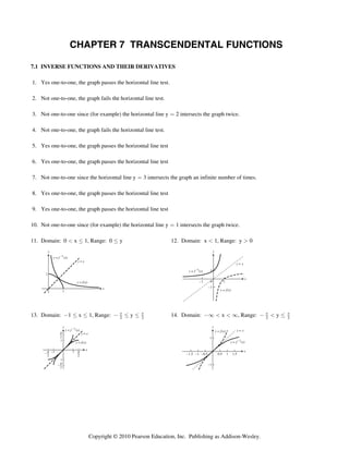
11. Domain: 0 x Ÿ 1, Range: 0 Ÿ y 12. Domain: x 1, Range: y € 0

13. Domain: c1 Ÿ x Ÿ 1, Range: c 1 Ÿ y Ÿ
#
1
# 14. Domain: c_ x _, Range: c 1 y Ÿ
#
1
#

Copyright © 2010 Pearson Education, Inc. Publishing as Addison-Wesley.

390 Chapter 7 Transcendental Functions

15. Domain: 0 Ÿ x Ÿ 6, Range: 0 Ÿ y Ÿ 3 16. Domain: c2 Ÿ x Ÿ 1, Range: c 1 Ÿ y 3

17. The graph is symmetric about y œ x.

(b) y œ È1 c x# Ê y# œ 1 c x# Ê x# œ 1 c y# Ê x œ È1 c y# Ê y œ È1 c x# œ f c" (x)

18. The graph is symmetric about y œ x.

" " "
yœ x Ê xœ y Ê yœ x œ f c" (x)

19. Step 1: y œ x# b 1 Ê x# œ y c 1 Ê x œ Èy c 1
Step 2: y œ Èx c 1 œ f c" (x)

20. Step 1: y œ x# Ê x œ cÈy, since x Ÿ !.
Step 2: y œ cÈx œ f c" (x)

21. Step 1: y œ x$ c 1 Ê x$ œ y b 1 Ê x œ (y b 1)"Î$
Step 2: y œ $ x b 1 œ f c" (x)
È

22. Step 1: y œ x# c 2x b 1 Ê y œ (x c 1)# Ê Èy œ x c 1, since x 1 Ê x œ 1 b Èy
Step 2: y œ 1 b Èx œ f c" (x)

23. Step 1: y œ (x b 1)# Ê Èy œ x b 1, since x c1 Ê x œ Èy c 1
Step 2: y œ Èx c 1 œ f c" (x)

24. Step 1: y œ x#Î$ Ê x œ y$Î#
Step 2: y œ x$Î# œ f c" (x)


Section 7.1 Inverse Functions and Their Derivatives 391

25. Step 1: y œ x& Ê x œ y"Î&
Step 2: y œ Èx œ f c" (x);
5

Domain and Range of f c" : all reals;
& "Î&
f af c" (x)b œ ˆx"Î& ‰ œ x and f c" (f(x)) œ ax& b œx

26. Step 1: y œ x% Ê x œ y"Î%
Step 2: y œ % x œ f c" (x);
È
Domain of f c" : x 0, Range of f c" : y 0;
% "Î%
f af c" (x)b œ ˆx"Î% ‰ œ x and f c" (f(x)) œ ax% b œx

27. Step 1: y œ x$ b 1 Ê x$ œ y c 1 Ê x œ (y c 1)"Î$
Step 2: y œ $ x c 1 œ f c" (x);
È
$ "Î$ "Î$
f af c" (x)b œ ˆ(x c 1)"Î$ ‰ b 1 œ (x c 1) b 1 œ x and f c" (f(x)) œ aax$ b 1b c 1b œ ax$ b œx

" "
28. Step 1: y œ # xc 7
# Ê # xœyb 7
# Ê x œ 2y b 7
c"
Step 2: y œ 2x b 7 œ f (x);
f af c" (x)b œ " (2x b 7) c 7 œ ˆx b 7 ‰ c
# # #
7
# œ x and f c" (f(x)) œ 2 ˆ " x c 7 ‰ b 7 œ (x c 7) b 7 œ x
# #

" " "
29. Step 1: y œ x # Ê x# œ y Ê xœ Èy
"
Step 2: y œ Èx œ f c" (x)
Domain of f c" : x € 0, Range of f c" : y € 0;
f af c" (x)b œ " œ " œ x and f c" (f(x)) œ
#
"
œ "
œ x since x € 0
Š "
‹ Šx‹ "
Éx "
Šx‹
"
È x
#

" " "
30. Step 1: y œ x $ Ê x$ œ y Ê xœ y $Î"

"
Step 2: y œ x $Î" œ É " œ f c" (x);
3
x
c"
Domain of f : x Á 0, Range of f c" : y Á 0;
" " " c"Î$ " c"
f af c" axbb œ $ $Î"c œ x "c œ x and f c" afaxbb œ ˆ x ‰ $ œ ˆx‰ œx
ax b

xb3 2y b 3
31. Step 1: y œ x c 2 Ê yax c 2b œ x b 3 Ê x y c 2y œ x b 3 Ê x y c x œ 2y b 3 Ê x œ yc1
b
Step 2: y œ 2xc 13 œ f c1 axb;
x
c"
Domain of f : x Á 1, Range of f c" : y Á 2;
1 b3 2 b3
ˆ 2x b 3‰
a2x b 3b b 3ax c 1b 2ˆ x
b 3‰
2 ax b 3 b b 3 a x c 2 b
f af c" axbb œ x c œ a2x b 3b c 2ax c 1b œ 5x
œ x and f c" afaxbb œ x
c œ ax b 3 b c ax c 2 b œ 5x
œx
1 c2 2 c1
ˆ 2x
x
b
c
3‰ 5 ˆxx
b
c
3‰ 5

Èx 2
32. Step 1: y œ Èx c 3 Ê yˆÈx c 3‰ œ Èx Ê yÈx c 3y œ Èx Ê yÈx c Èx œ 3y Ê x œ Š y 3y 1 ‹
c
2
Step 2: y œ ˆ x 3x 1 ‰ œ f c1 axb;
c
Domain of f c" : Ðc_, 0Ó r a1, _b, Range of f c" : Ò0, 9Ñ r a9, _b;
Éˆ x 3x 1 ‰2 Éˆ x 3x 1 ‰2 3x
f af c" axbb œ c
; If x € 1 or x Ÿ 0 Ê 3x
xc1 0Ê c
œ x 1c œ 3x
3x c 3ax c 1b œ 3x
œ x and
x 1 c3
2 2 3x 3
Éˆ x 3x 1 ‰ c 3
c Éˆ x 3x 1 ‰ c 3
c c
È x
2
3Š ‹
c"
f afaxbb œ : c È x 3
œ 9x
œ 9x
œx
‹c1; ˆÈ x c ˆÈ x c 3 ‰‰ 2
Š
È x 9
c È
x 3



33. Step 1: y œ x2 c 2x, x Ÿ 1 Ê y b 1 œ ax c 1b2 , x Ÿ 1 Ê cÈy b 1 œ x c 1, x Ÿ 1 Ê x œ 1 c Èy b 1
Step 2: y œ 1 c Èx b 1 œ f c1 axb;
Domain of f c" : Òc1, _Ñ, Range of f c" : Ðc_, 1Ó;
2
f af c" axbb œ Š1 c Èx b 1‹ c 2Š1 c Èx b 1‹ œ 1 c 2Èx b 1 b x b 1 c 2 b 2Èx b 1 œ x and

f c" afaxbb œ 1 c Èax2 c 2xb b 1, x Ÿ 1 œ 1 c Éax c 1b2 , x Ÿ 1 œ 1 c lx c 1l œ 1 c a1 c xb œ x

1 Î5 y5 c 1 5 c1
34. Step 1: y œ a2x3 b 1b Ê y5 œ 2x3 b 1 Ê y5 c 1 œ 2x3 Ê 2 œ x3 Ê x œ É y
3
2
c1
Step 2: y œ É x œ f c 1 ax b ;
3 5
2
Domain of f c" : ac_, _b, Range of f c" : ac_, _b;
3 1 Î5 1 Î5
c1 c1 1 Î5 1 Î5
f af c" axbb œ Œ2ŠÉ x
5
b 19 œ Š 2Š x b 1‹ œ aax5 c 1b b 1b œ ax5 b œ x and
3 5
2 ‹ 2 ‹

5
1 5
’a2x3 b1b “ c 1
Î
3
b 1 bc 1
f c" afaxbb œ Ê
3
œ É a2x œ É 2x œ x
3 3 3
2 2 2

35. (a) y œ 2x b 3 Ê 2x œ y c 3 (b)
Ê x œ y c 3 Ê f c" (x) œ
# #
x
# c 3
#
"
œ 2, œ
"c
df ¸ df
(c) dx x cœ 1 dx ¹ #
x 1
œ

" "
36. (a) y œ 5 xb7 Ê 5 xœyc7 (b)
c"
Ê x œ 5y c 35 Ê f (x) œ 5x c 35
" df
œ œ5
"c
df ¸
(c) dx x cœ 1 5 , dx ¹
x &Î%$œ

37. (a) y œ 5 c 4x Ê 4x œ 5 c y (b)
Ê x œ 5 c y Ê f c" (x) œ
4 4
5
4 c x
4
"
œ c4, œc
"c
df ¸ df
(c) dx x 1 #Î œ dx ¹ 4
x 3
œ

"
38. (a) y œ 2x# Ê x# œ # y (b)
" c"
Ê xœ È2
Èy Ê f (x) œ Èx
#

(c) df ¸
dx x &œ
œ 4xk x 5
œ œ 20,
" "
œ xc"Î# ¹ œ
"c
df
dx ¹ #È 2 #0
x &œ 0 x 50œ


$
39. (a) f(g(x)) œ ˆÈx‰ œ x, g(f(x)) œ Èx3 œ x
3 3
(b)
w # w w
(c) f (x) œ 3x Ê f (1) œ 3, f (c1) œ 3;
" " "
gw (x) œ 3 xc#Î$ Ê gw (1) œ 3 , gw (c1) œ 3
(d) The line y œ 0 is tangent to f(x) œ x$ at (!ß !);
the line x œ 0 is tangent to g(x) œ $ x at (0ß 0)
È

40. (a) h(k(x)) œ "
4
ˆ(4x)"Î$ ‰$ œ x, (b)
"Î$
k(h(x)) œ Š4 † x
œx
$
4 ‹
(c) hw (x) œ w w
4 Ê h (2) œ 3, h (c2)
3x
œ 3;
#

k (x) œw 4
3 (4x)
c#Î$
Ê kw (2) œ " ,
3 kw (c2) œ "
3
(d) The line y œ 0 is tangent to h(x) œ x
at (!ß !);
$
4
the line x œ 0 is tangent to k(x) œ (4x)"Î$ at
(!ß !)

" " " "
œ 3x# c 6x Ê œ œ œ 2x c 4 Ê œ œ
df df "c df df "c
41. dx dx ¹ df º 9 42. dx dx ¹ df º 6
x œ f(3) dx x œ f(5) dx
x œ 3 x œ 5

" " "c "c " "
œ œ œ œ3 dg
œ dg
œ œ
"c
df "c
df
43. dx ¹ dx ¹ df º ˆ3‰
" 44. dx ¹ dx ¹ dg º 2
x œ 4 x œ f(2) dx x œ 0 x œ f(0) dx
x œ 2 x œ 0

" "
45. (a) y œ mx Ê x œ m y Ê f c" (x) œ m x
c" "
(b) The graph of y œ f (x) is a line through the origin with slope m.

" "
46. y œ mx b b Ê x œ y
m c b
m Ê f c" (x) œ m xc b
m; the graph of f c" (x) is a line with slope m and y-intercept c m .
b

47. (a) y œ x b 1 Ê x œ y c 1 Ê f c" (x) œ x c 1
(b) y œ x b b Ê x œ y c b Ê f c" (x) œ x c b
(c) Their graphs will be parallel to one another and lie on
opposite sides of the line y œ x equidistant from that
line.

48. (a) y œ cx b 1 Ê x œ cy b 1 Ê f c" (x) œ 1 c x;
the lines intersect at a right angle
(b) y œ cx b b Ê x œ cy b b Ê f c" (x) œ b c x;
the lines intersect at a right angle
(c) Such a function is its own inverse.



49. Let x" Á x# be two numbers in the domain of an increasing function f. Then, either x" x# or
x" € x# which implies f(x" ) f(x# ) or f(x" ) € f(x# ), since f(x) is increasing. In either case,
f(x" ) Á f(x# ) and f is one-to-one. Similar arguments hold if f is decreasing.

" " " "
50. f(x) is increasing since x# € x" Ê x# b € x" b 5 ; œ Ê œ œ3
5 df "c
df
3 6 3 6 dx 3 dx ˆ3‰
"

" "
51. f(x) is increasing since x# € x" Ê 27x$ € 27x" ; y œ 27x$ Ê x œ
#
$
3 y"Î$ Ê f c" (x) œ 3 x"Î$ ;
" " "
œ 81x# Ê œ œ œ xc#Î$
df "c
df
dx dx 81x # ¸1 9
3 x $Î" 9x $Î#

" "
52. f(x) is decreasing since x# € x" Ê 1 c 8x$ 1 c 8x" ; y œ 1 c 8x$ Ê x œ
#
$
# (1 c y)"Î$ Ê f c" (x) œ # (1 c x)"Î$ ;
" c"
œ c24x# Ê œ œ œ c " (1 c x)c#Î$
"c
df df ¸1
dx dx c24x #
2 1 x
ÑcÐ $Î" 6(" c x) $Î# 6

53. f(x) is decreasing since x# € x" Ê (1 c x# )$ (1 c x" )$ ; y œ (1 c x)$ Ê x œ 1 c y"Î$ Ê f c" (x) œ 1 c x"Î$ ;
" c"
œ c3(1 c x)# Ê œ œ œ c " xc#Î$
"c
df df
dx dx c3(1 c x) # ¹ 3x $Î# 3
1 x
c $Î"

&Î$ &Î$
54. f(x) is increasing since x# € x" Ê x# € x" ; y œ x&Î$ Ê x œ y$Î& Ê f c" (x) œ x$Î& ;
"
œ x#Î$ Ê œ œ œ xc#Î&
"c
df 5 df 3 3
dx 3 dx 5
x $Î# ¹ 5x &Î# 5
3 x &Î$

55. The function g(x) is also one-to-one. The reasoning: f(x) is one-to-one means that if x" Á x# then f(x" ) Á f(x# ), so
cf(x" ) Á cf(x# ) and therefore g(x" ) Á g(x# ). Therefore g(x) is one-to-one as well.

56. The function h(x) is also one-to-one. The reasoning: f(x) is one-to-one means that if x" Á x# then f(x" ) Á f(x# ), so
" "
f(x ) Á f(x ) , and therefore h(x" ) Á h(x# ).
" #

57. The composite is one-to-one also. The reasoning: If x" Á x# then g(x" ) Á g(x# ) because g is one-to-one. Since
g(x" ) Á g(x# ), we also have f(g(x" )) Á f(g(x# )) because f is one-to-one. Thus, f ‰ g is one-to-one because
x" Á x# Ê f(g(x" )) Á f(g(x# )).

58. Yes, g must be one-to-one. If g were not one-to-one, there would exist numbers x" Á x# in the domain of g with
g(x" ) œ g(x# ). For these numbers we would also have f(g(x" )) œ f(g(x# )), contradicting the assumption that
f ‰ g is one-to-one.

59. (g ‰ f)(x) œ x Ê g(f(x)) œ x Ê gw (f(x))f w (x) œ 1

60. W(a) œ 'f(a) 1 ’af c" (y)b c a# “ dy œ 0 œ 'a 21x[f(a) c f(x)] dx œ S(a); Ww (t) œ 1’af c" (f(t))b c a# “ f w (t)
f(a) a
# #

œ 1 at# c a# b f w (t); also S(t) œ 21f(t)'a x dx c 21'a xf(x) dx œ c1f(t)t# c 1f(t)a# d c 21'a xf(x) dx Ê Sw (t)
t t t

œ 1t# f w (t) b 21tf(t) c 1a# f w (t) c 21tf(t) œ 1 at# c a# b f w (t) Ê Ww (t) œ Sw (t). Therefore, W(t) œ S(t) for all t − [aß b].

61-68. Example CAS commands:
Maple:
with( plots );#63
f := x -> sqrt(3*x-2);
domain := 2/3 .. 4;
x0 := 3;
Df := D(f); # (a)



plot( [f(x),Df(x)], x=domain, color=[red,blue], linestyle=[1,3], legend=["y=f(x)","y=f '(x)"],
title="#61(a) (Section 7.1)" );
q1 := solve( y=f(x), x ); # (b)
g := unapply( q1, y );
m1 := Df(x0); # (c)
t1 := f(x0)+m1*(x-x0);
y=t1;
m2 := 1/Df(x0); # (d)
t2 := g(f(x0)) + m2*(x-f(x0));
y=t2;
domaing := map(f,domain); # (e)
p1 := plot( [f(x),x], x=domain, color=[pink,green], linestyle=[1,9], thickness=[3,0] ):
p2 := plot( g(x), x=domaing, color=cyan, linestyle=3, thickness=4 ):
p3 := plot( t1, x=x0-1..x0+1, color=red, linestyle=4, thickness=0 ):
p4 := plot( t2, x=f(x0)-1..f(x0)+1, color=blue, linestyle=7, thickness=1 ):
p5 := plot( [ [x0,f(x0)], [f(x0),x0] ], color=green ):
display( [p1,p2,p3,p4,p5], scaling=constrained, title="#63(e) (Section 7.1)" );
Mathematica: (assigned function and values for a, b, and x0 may vary)
If a function requires the odd root of a negative number, begin by loading the RealOnly package that allows Mathematica
to do this. See section 2.5 for details.
<<Miscellaneous `RealOnly`
Clear[x, y]
{a,b} = {c2, 1}; x0 = 1/2 ;
f[x_] = (3x b 2) / (2x c 11)
Plot[{f[x], f'[x]}, {x, a, b}]
solx = Solve[y == f[x], x]
g[y_] = x /. solx[[1]]
y0 = f[x0]
ftan[x_] = y0 b f'[x0] (x-x0)
gtan[y_] = x0 b 1/ f'[x0] (y c y0)
Plot[{f[x], ftan[x], g[x], gtan[x], Identity[x]},{x, a, b},
Epilog Ä Line[{{x0, y0},{y0, x0}}], PlotRange Ä {{a,b},{a,b}}, AspectRatio Ä Automatic]

69-70. Example CAS commands:
Maple:
with( plots );
eq := cos(y) = x^(1/5);
domain := 0 .. 1;
x0 := 1/2;
f := unapply( solve( eq, y ), x ); # (a)
Df := D(f);
plot( [f(x),Df(x)], x=domain, color=[red,blue], linestyle=[1,3], legend=["y=f(x)","y=f '(x)"],
title="#70(a) (Section 7.1)" );
q1 := solve( eq, x ); # (b)
g := unapply( q1, y );
m1 := Df(x0); # (c)
t1 := f(x0)+m1*(x-x0);
y=t1;
m2 := 1/Df(x0); # (d)



t2 := g(f(x0)) + m2*(x-f(x0));
y=t2;
domaing := map(f,domain); # (e)
p1 := plot( [f(x),x], x=domain, color=[pink,green], linestyle=[1,9], thickness=[3,0] ):
p2 := plot( g(x), x=domaing, color=cyan, linestyle=3, thickness=4 ):
p3 := plot( t1, x=x0-1..x0+1, color=red, linestyle=4, thickness=0 ):
p4 := plot( t2, x=f(x0)-1..f(x0)+1, color=blue, linestyle=7, thickness=1 ):
p5 := plot( [ [x0,f(x0)], [f(x0),x0] ], color=green ):
display( [p1,p2,p3,p4,p5], scaling=constrained, title="#70(e) (Section 7.1)" );
Mathematica: (assigned function and values for a, b, and x0 may vary)
For problems 69 and 70, the code is just slightly altered. At times, different "parts" of solutions need to be used, as in the
definitions of f[x] and g[y]
Clear[x, y]
{a,b} = {0, 1}; x0 = 1/2 ;
eqn = Cos[y] == x1/5
soly = Solve[eqn, y]
f[x_] = y /. soly[[2]]
Plot[{f[x], f'[x]}, {x, a, b}]
solx = Solve[eqn, x]
g[y_] = x /. solx[[1]]
y0 = f[x0]
ftan[x_] = y0 b f'[x0] (x c x0)
gtan[y_] = x0 b 1/ f'[x0] (y c y0)
Plot[{f[x], ftan[x], g[x], gtan[x], Identity[x]},{x, a, b},
Epilog Ä Line[{{x0, y0},{y0, x0}}], PlotRange Ä {{a, b}, {a, b}}, AspectRatio Ä Automatic]

7.2 NATURAL LOGARITHMS

1. (a) ln 0.75 œ ln 3
4 œ ln 3 c ln 4 œ ln 3 c ln 2# œ ln 3 c 2 ln 2
(b) ln 4
9 œ ln 4 c ln 9 œ ln 2# c ln 3# œ 2 ln 2 c 2 ln 3
"
(c) ln œ ln 1 c ln 2 œ c ln 2
# (d) ln È9 œ " ln 9 œ
3
3
"
3 ln 3# œ 2
3 ln 3
(e) ln 3È2 œ ln 3 b ln 2"Î# œ ln 3 b " ln 2
#
(f) ln È13.5 œ " ln 13.5 œ " ln 27 œ " aln 3$ c ln 2b œ " (3 ln 3 c ln 2)
# # # # #

"
2. (a) ln 125 œ ln 1 c 3 ln 5 œ c3 ln 5 (b) ln 9.8 œ ln 49
5 œ ln 7# c ln 5 œ 2 ln 7 c ln 5
(c) ln 7È7 œ ln 7$Î# œ 3
# ln 7 (d) ln 1225 œ ln 35# œ 2 ln 35 œ 2 ln 5 b 2 ln 7
ln 35 b ln ln 5 b ln 7 c ln 7 "
œ ln 7 c ln 5$ œ ln 7 c 3 ln 5
"
(e) ln 0.056 œ ln 7
125 (f) ln 25
7
œ # ln 5 œ #

3. (a) ln sin ) c ln ˆ sin ) ‰ œ ln : sin )
œ ln 5 " c
(b) ln a3x# c 9xb b ln ˆ 3x ‰ œ ln Š 3x 3x 9x ‹ œ ln (x c 3)
#
5 Š sin ‹ ;
)
5

"
ln a4t% b c ln 2 œ ln È4t% c ln 2 œ ln 2t# c ln 2 œ ln Š 2t ‹ œ ln at# b
#
(c) # #

4. (a) ln sec ) b ln cos ) œ ln [(sec ))(cos ))] œ ln 1 œ 0
b
(b) ln (8x b 4) c ln 2# œ ln (8x b 4) c ln 4 œ ln ˆ 8x 4 4 ‰ œ ln (2x b 1)
"Î$
(c) 3 ln Èt# c 1 c ln (t b 1) œ 3 ln at# c 1b c ln (t b 1) œ 3 ˆ " ‰ ln at# c 1b c ln (t b 1) œ ln Š (t b(t1)(t1) ") ‹
c
$

3 b

œ ln (t c 1)


Section 7.2 Natural Logarithms 397
" " "
5. y œ ln 3x Ê yw œ ˆ 3x ‰ (3) œ
1
x 6. y œ ln kx Ê yw œ ˆ kx ‰ (k) œ x

7. y œ ln at# b Ê dy
dt œ ˆ t" ‰ (2t) œ#
2
t 8. y œ ln ˆt$Î# ‰ Ê dy
dt œ ˆ t " ‰ ˆ 3 t"Î# ‰ œ
#Î$#
3
2t

9. y œ ln 3
x œ ln 3xc" Ê dy
dx œ ˆ 3x" ‰ ac3xc# b œ c x
"c
"

" "
10. y œ ln 10
x œ ln 10xc" Ê dy
dx œ ˆ 10x ‰ ac10xc# b œ c x
"c

" "
11. y œ ln () b 1) Ê dy
d) œ ˆ ) b 1 ‰ (1) œ )b1 12. y œ ln (2) b 2) Ê dy
d) œ ˆ #) " 2 ‰ (2) œ
b
"
)b1

"
13. y œ ln x$ Ê dy
œ ˆ x ‰ a3x# b œ 14. y œ (ln x)$ Ê dy
œ 3(ln x)# † (ln x) œ 3(ln x)
#
3 d
dx $ x dx dx x

15. y œ t(ln t)# Ê dy
dt œ (ln t)# b 2t(ln t) † d
dt (ln t) œ (ln t)# b 2t ln t
t œ (ln t)# b 2 ln t

16. y œ tÈln t œ t(ln t)"Î# Ê œ (ln t)"Î# b " t(ln t)c"Î# † (ln t) œ (ln t)"Î# b
#Î"c
dy d t(ln t)
dt # dt #t
"
œ (ln t)"Î# b #(ln t) #Î"

"
17. y œ x
ln x c x
Ê dy
œ x$ ln x b x
† c 4x
œ x$ ln x
% % % $
4 16 dx 4 x 16

4 3
18. y œ ax2 ln xb Ê dy
dx œ 4ax2 ln xb ˆx2 † 1
x b 2x ln x‰ œ 4x6 aln xb3 ax b 2x ln xb œ 4x7 aln xb3 b8x7 aln xb4

t ˆ t ‰ c (ln t)(1)
"
1 c ln t
19. y œ ln t
t Ê dy
dt œ t # œ t #

" b ln t t ˆ t ‰ c (" b ln t)(1)
"
" c 1 c ln t
20. y œ t Ê dy
dt œ t # œ t # œ c ln t
t #

(1 b ln x) ˆ x ‰ c (ln x) ˆ x ‰
" " "
b lnxx c lnxx "
21. y œ ln x
1 b ln x Ê yw œ (1 b ln x) # œ x
(1 b ln x) # œ x(1 b ln x) #

(1bln x) ˆln x b x† x ‰ c (x ln x) ˆ x ‰
" "
(" b ln x) c ln x
22. y œ Ê yw œ œ œ1c
#
x ln x ln x
1 b ln x (1bln x) # (1 b ln x) # (1 b ln x) #

23. y œ ln (ln x) Ê yw œ ˆ ln"x ‰ ˆ " ‰ œ
x
"
x ln x

" " " "
24. y œ ln (ln (ln x)) Ê yw œ ln (ln x) † d
dx (ln (ln x)) œ ln (ln x) † ln x † d
dx (ln x) œ x (ln x) ln (ln x)

"
25. y œ )[sin (ln )) b cos (ln ))] Ê dy
d) œ [sin (ln )) b cos (ln ))] b ) <cos (ln )) † ) c sin (ln )) † " ‘
)
œ sin (ln )) b cos (ln )) b cos (ln )) c sin (ln )) œ 2 cos (ln ))

sec ) tan ) b sec ) sec )(tan ) b sec ))
26. y œ ln (sec ) b tan )) Ê dy
œ œ œ sec )
#
d) sec ) b tan ) tan ) b sec )

27. y œ ln "
xÈ x b 1
œ c ln x c "
# ln (x b 1) Ê yw œ c x c # ˆ x b 1 ‰ œ c 2(x b 1) b x œ c 2x(xb 21)
" " "
2x(x b 1)
3x
b

" 1bx " " " " "
28. y œ # ln 1cx œ # cln (1 b x) c ln (1 c x)d Ê yw œ #
< 1 b x c ˆ 1 c x ‰ (c1)‘ œ # ’ (1c xx)("1c x) “ œ
1
b
b bx "
1cx #



1 b ln t (1cln t) ˆ t ‰ c (1 b ln t) ˆ
" "c ‰ " c lnt t b t b lnt t
"
29. y œ 1 c ln t Ê dy
dt œ (1 c ln t) #
t
œ t
(1 c ln t) # œ 2
t(1 c ln t) #

"Î#
30. y œ Éln Èt œ ˆln t"Î# ‰ Ê dy
dt œ "
#
ˆln t"Î# ‰c"Î# † d
dt
ˆln t"Î# ‰ œ "
#
ˆln t"Î# ‰c"Î# † "
† d
dt
ˆt"Î# ‰
t#Î"

œ "
#
ˆln t"Î# ‰c"Î# † " "
† # tc"Î# œ "
t
#Î"
4tÉln Èt

" sec (ln )) tan (ln )) tan (ln ))
31. y œ ln (sec (ln ))) Ê dy
d) œ sec (ln )) † d
d) (sec (ln ))) œ sec (ln )) † d
d) (ln )) œ )

Èsin ) cos ) 2
" " ) sin ) ‰
32. y œ ln 1 b 2 ln ) œ # (ln sin ) b ln cos )) c ln (1 b 2 ln )) Ê dy
d) œ #
ˆ cos ) c
sin cos ) c )
1 b # ln )
"
œ # ’cot ) c tan ) c 4
)(1 b 2 ln )) “

x b1 " 5†2x " " "
&
33. y œ ln Š aÈ1 c b ‹ œ 5 ln ax# b 1b c ln (1 c x) Ê yw œ c # ˆ 1 c x ‰ (c1) œ b
#
10x
x # x b1# x b1
# #(1 c x)

(x b 1)
34. y œ ln É (x b 2) œ "
[5 ln (x b 1) c 20 ln (x b 2)] Ê yw œ " ˆxb1 c
5 20 ‰
œ 5
’ (x(x b 1)(x bb 1) “
b 2) c 4(x
&
!# # # xb# # 2)
3x b
œ c 5 ’ (x b 1)(x2 #) “
# b

35. y œ 'x
x #

ln Èt dt Ê dy
œ Šln Èx# ‹ † d
ax# b c Šln É x ‹ † d
Š x ‹ œ 2x ln kxk c x ln
kx k
# #

Î# 2 dx dx # dx # È2

36. y œ '
Èx
3
" "
ˆÈx‰ œ ˆln Èx‰ ˆ 3 xc#Î$ ‰ c ˆln Èx‰ ˆ # xc"Î# ‰
È x
ln t dt Ê dy
dx œ ˆln Èx‰ †
3 d
dx
ˆÈx‰ c ˆln Èx‰ †
3 d
dx
3

ln Èx
3 ln Èx
œ c
3È x2 2È x
3

37. 'c
c
3
2
"
x dx œ cln kxkd c# œ ln 2 c ln 3 œ ln
c$
2
3 38. ' 01 3x3c# dx œ cln k3x c 2kd ! œ ln 2 c ln 5 œ ln 5
c c"
2

39. ' y 2y25 dy œ ln ky# c 25k b C
c # 40. ' 4r8r 5 dr œ ln k4r# c 5k b C
c #

41. '0 1
sin t
2ccos t
1
dt œ cln k2 c cos tkd ! œ ln 3 c ln 1 œ ln 3; or let u œ 2 c cos t Ê du œ sin t dt with t œ 0

Ê u œ 1 and t œ 1 Ê u œ 3 Ê '0 dt œ '1
3
du œ cln kukd $ œ ln 3 c ln 1 œ ln 3
1
sin t "
2ccos t u "

42. '0 Î1 3
4 sin )
1c4 cos ) d) œ cln k1 c 4 cos )kd !
1Î$
œ ln k1 c 2k œ c ln 3 œ ln " ; or let u œ 1 c 4 cos ) Ê du œ 4 sin ) d)
3

Ê u œ c1 Ê '0 d) œ '
3 c 1
du œ cln kukd c" œ c ln 3 œ ln
Î1
1 4 sin ) " "
with ) œ 0 Ê u œ c3 and ) œ 3 1c4 cos ) 3
c u c$ 3

"
43. Let u œ ln x Ê du œ x dx; x œ 1 Ê u œ 0 and x œ 2 Ê u œ ln 2;
'1 2
2 ln x
x dx œ '0
ln 2
2u du œ cu# d 0 œ (ln 2)#
ln 2

"
44. Let u œ ln x Ê du œ x dx; x œ 2 Ê u œ ln 2 and x œ 4 Ê u œ ln 4;
'2 4
dx
x ln x œ 'ln 2
ln 4
"
u du œ cln ud ln 4 œ ln (ln 4) c ln (ln 2) œ ln ˆ ln 4 ‰ œ ln Š ln 2 ‹ œ ln ˆ 2ln 22 ‰ œ ln 2
ln 2 ln 2 ln 2
ln #


Section 7.2 Natural Logarithms 399
"
'2 4
dx
x(ln x) # œ 'ln 2 uc# du œ <c " ‘ ln 2 œ c ln"4 b
ln 4

u
ln 4 "
ln # œ c ln"# b #
"
ln 2
"
œ c 2 ln # b "
ln # œ "
# ln 2 œ "
ln 4

"
'2 16
dx
œ "
#
'ln 2 ln 16
uc"Î# du œ <u"Î# ‘ ln 2 œ Èln 16 c Èln 2 œ È4 ln 2 c Èln 2 œ 2Èln 2 c Èln 2 œ Èln 2
ln 16
2xÈln x

47. Let u œ 6 b 3 tan t Ê du œ 3 sec# t dt;
' 6 3 sectant t dt œ ' du œ ln kuk b C œ ln k6 b 3 tan tk b C
b3
#
u

48. Let u œ 2 b sec y Ê du œ sec y tan y dy;
' secbysec yy dy œ ' du œ ln kuk b C œ ln k2 b sec yk b C
#
tan
u

49. Let u œ cos x
# Ê du œ c " sin
#
x
# dx Ê c2 du œ sin x
# dx; x œ 0 Ê u œ 1 and x œ 1
# Ê uœ "
È2 ;

'0 dx œ '0 dx œ c2 '1
Î1 2 Î12
sin x 1 ÈÎ 2 ÈÎ "
tan x
# cos x
# du
u œ cc2 ln kukd 1
1
2
œ c2 ln È2 œ 2 ln È2 œ ln 2
#

1 " 1
50. Let u œ sin t Ê du œ cos t dt; t œ 4 Ê uœ È2 and t œ # Ê u œ 1;

'Î1
Î1

4
2
cot t dt œ ' Î1
Î1

4
2
cos t
sin t dt œ '1
1

ÈÎ 2
du
u œ cln kukd " È# œ c ln
"Î
"
È2 œ ln È2

) " ) ) 1 " È3
51. Let u œ sin 3 Ê du œ 3 cos 3 d) Ê 6 du œ 2 cos 3 d) ; ) œ # Ê uœ # and ) œ 1 Ê u œ # ;
' d) œ ' d) œ 6 '1 2
1 1 È 3 2
Î È3
)
c ln " ‹ œ 6 ln È3 œ ln 27
2 cos 3 ) È
Î1 2
2 cot 3 Î1 2 sin 3 )
Î
du
u œ 6 cln kukd 1 2 2 œ 6 Šln
3
Î
Î
# #

1 "
52. Let u œ cos 3x Ê du œ c3 sin 3x dx Ê c2 du œ 6 sin 3x dx; x œ 0 Ê u œ 1 and x œ 1# Ê uœ È2 ;

'0 6 tan 3x dx œ '0 dx œ c2 '1
Î1 12 Î112 1 ÈÎ 2 ÈÎ "
6 sin 3x
cos 3x
du
u œ c2 cln kukd 1
1
2
œ c2 ln È2 c ln 1 œ 2 ln È2 œ ln 2

53. ' dx
2Èx b 2x
œ' dx
2 È x ˆ1 b È x ‰
; let u œ 1 b Èx Ê du œ "
#È x
dx; ' 2Èx ˆdxb Èx‰ œ '
1
du
u œ ln kuk b C
œ ln ¸1 b Èx¸ b C œ ln ˆ1 b Èx‰ b C

54. Let u œ sec x b tan x Ê du œ asec x tan x b sec# xb dx œ (sec x)(tan x b sec x) dx Ê sec x dx œ du
u ;

' sec x dx
Èln (sec x b tan x) œ' du
uÈln u
œ ' (ln u)c"Î# † "
u du œ 2(ln u)"Î# b C œ 2Èln (sec x b tan x) b C

" " "
55. y œ Èx(x b 1) œ (x(x b 1))"Î# Ê ln y œ ln (x(x b 1)) Ê 2 ln y œ ln (x) b ln (x b 1) Ê 2y
œ b
w

# y x x b1
Èx(x b 1) (2x b 1)
Ê yw œ ˆ " ‰ Èx(x b 1) ˆ x b
#
" " ‰
x b1 œ 2x(x b 1) œ 2x b "
2Èx(x b 1)

" "
56. y œ Èax# b 1b (x c 1)# Ê ln y œ cln ax# b 1b b 2 ln (x c 1)d Ê y
œ ˆ x 2x 1 b 2 ‰
w

# y # # b xc1
" ‰ a2x c x b 1b kx c 1k
Ê yw œ Èax# +1b (x c 1)# ˆ x b œ Èax# b 1b (x c 1)# ’ ax c x1b(x c 1) “ œ
x b1
#
x x # #
# b1 xc1 b b # Èx b 1 (x c 1)
#

"Î# " " dy "
57. y œ É t b 1 œ ˆ t b 1 ‰
t t
Ê ln y œ # [ln t c ln (t b 1)] Ê y dt œ #
ˆ" c
t
" ‰
tb1

"
Ê dy
dt œ # Étb1 ˆ" c
t
t
" ‰
tb1 œ "
#
t "
É t b 1 ’ t(t b 1) “ œ "
2Èt (t b 1) #Î$


Chp7 transcendental functions

Recommended

Recommended

More Related Content

Featured

Featured (20)

Chp7 transcendental functions