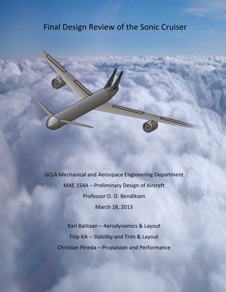
1. Final Design Review of the Sonic Cruiser
UCLA Mechanical and Aerospace Engineering Department
MAE 154A – Preliminary Design of Aircraft
Professor O. O. Bendiksen
March 18, 2013
Karl Balitaan – Aerodynamics & Layout
Filip Kik – Stability and Trim & Layout
Christian Pineda – Propulsion and Performance
1

2. Table of Contents
I.
II.
Introduction – pg 5
Summary of Sonic Cruiser Specifications – pg 6
III.
Aircraft Design and Layout – pg 7-17
IV.
V.
Aerodynamics – pg 18-35
Propulsion and Performance – pg 36-50
VI.
Stability and Trim – pg 51-63
VII.
Conclusions – pg 64-65
VIII.
References – pg 66
IX.
Appendix – pg 67-74
2

3. List of Figures and Tables
Aircraft Design & Layout
Table D1 - Final Weight Breakdown for Aquila, our Optimized Sonic Cruiser at Load Condition I – pg 9
Table D.2 - Fuselage Exterior Dimensions – pg 10
Table D3 - Fuselage’s Nose Section – pg 10
Table D4 - Fuselage’s Center Section – pg 10
Table D5 - Fuselage’s Tail Section – pg 11
Table D6 - Fuselage Dimensions – pg 11
Table D7 - Fuel Tank Capacity of Aquila – pg 12
Table D8 - Summary of Aircraft Weight and CG for Load Condition I – pg 13
Table D9 - Summary of Aircraft Weight and CG for Load Condition II – pg 13
Table D10 - Summary of Aircraft Weight and CG for Load Condition III – pg 13
Table D11 - Summary of Aircraft Weight and CG for Load Condition IV – pg 13
Figure D1 – Aquila Seating Layout – pg 14
Figure D2 – Fuselage Cross Section Interior View – pg 15
Figure D3 – Front View of Aquila with Landing Gears Deployed – pg 16
Figure D4 – Front View of Aquila with Landing Gears Retracted – pg 16
Figure D5 – Side View of Aquila with Landing Gears Deployed – pg 16
Figure D6 – Side View of Aquila with Landing Gears Retracted – pg 17
Figure D7 – Top View of Aquila – pg 17
Aerodynamics:
Table A1 - Initial CFD Code Parameter Sweeps for 0.95Ma and CL = 0.3 – pg 19
Table A2 - Possible Optimized Wing Configuration – pg 20
Table A3 - Wing A Fixed Geometric Relationships – pg 21
Table A4 - Starting Cruise Conditions for Sonic Cruiser – pg 22
Table A5 - NACA 64-006 Lift Polar – pg 23
Table A6 - NACA 64-006 Drag Polar – Parasite Drag Formula – pg 23
Table A7 - Planform Area Summary – pg 24
Table A8 - Sonic Cruiser’s Optimized Wing Geometry Relationships – pg 25
Table A9 - Optimized Wing Dimensions – pg 25
Table A10 - Aileron Dimensions – pg 25
Table A11 - Canard Dimensions – pg 26
Table A12 - Dimensions for 1 Vertical Stabilizer – pg 27
Table A13 - Rudder Dimensions – pg 27
Table A14 - Reynolds Number for Cruise Conditions at 0.95Ma – pg 27
Table A15 - Induced Drag Formula – pg 27
Table A16 - Total Drag Coefficient for the Sonic Cruiser’s Wing and Canard for CL = 0.3 – pg 28
Table A17 - Lift-to-Drag Ratio for Wing and Canard at Cruise Lift Coefficient of CL = 0.3 – pg 29
Table A18 - Fuselage Skin Friction Drag Coefficient – pg 30
Table A19 - Vertical Stabilizer Skin Friction Drag Coefficient – pg 30
Table A20 - External Geometry of Engine and Nacelles – pg 31
Table A21 - Properly-Designed Engine and Nacelle Skin Friction Drag Coefficient – pg 31
Table A22 - Total Aircraft Lift Coefficient for Cruise at CL = 0.3 for Load Condition I at Start of Cruise – pg 32
Table A23 - Aerodynamic Center and Moment Calculations with respect to MAC for C L = 0.3 – pg 34
Table A24 - Fowler Flaps Dimensions – pg 35
Table A25 - Maximum Lift Coefficients for Airfoil and Wing without Addition of Flaps – pg 35
Table A26 - Maximum Lift Coefficients for Airfoil and Wing with Addition of Flaps – pg 35
Table A27 - Parasite Drag Contribution from Fully Extended Fowler Flaps – pg 36
3

4. Figure A1 – Comparison of L/D vs. Ma between Baseline and Optimized Wing – pg 21
Figure A2 – Comparison of Drag Coefficient vs. Ma between Baseline and Optimized Wing – pg 22
Figure A3 – Comparison of total L/D vs. Ma between Baseline and Optimized Wing – pg 28
Figure A3 – Comparison of total Drag Coefficient vs. Ma between Baseline and Optimized Wing – pg 30
Performance:
Table P1 – GE90-94B Specifications – pg 37
Table P2 – Climb Performance – pg 44
Table P3 – Maximum Mach – pg 46
Table P4 – Absolute Ceiling – pg 46
Table P5 – Parameters in Determining Maximum Range – pg 47
Table P6 – Rate of Descent – pg 48
Table P7 – Fuel Weight Breakdown – pg 48
Table P8 – Performance Summary – pg 51
Figure P1 – Landing Gear Drag Coefficient Factor – pg 39
Figure P2 – Takeoff Parameters – pg 40
Figure P3 – Takeoff Performance – pg 41
Figure P4 – Takeoff Distance – pg 41
Figure P5 – Thrust Map Scaling: PW4056 to GE90-94B – pg 43
Figure P6 – Climb Altitude vs. Time – pg 44
Figure P7 – Climb Cruise Altitude Variation – pg 45
Figure P8 – Complete Mission Profile – pg 47
Figure P9 – Maximum Climb Performance Scaling from JTD9-7 – pg 49
Stability and Trim:
Table S1.a – CG Location for all Loading Conditions at Start of Cruise – pg 55
Table S1.b – CG Location for all Loading Conditions at Takeoff – pg 56
Table S1.c – CG Location for Load Condition I at End of Cruise and After Descent – pg 57
Tables S2 – Parameters and Respective Values for Calculation of Static Margin – pg 59-61
Table S3 – Static Margin and Pitch Stability for all Load Conditions and Flight Scenarios – pg 61
Tables S4 – Trim Calculations – pg 63
Figures S1: Plot of Pitch Stability for all Load Conditions at Start of Cruise and Takeoff – pg 62
Appendix:
Table AP1 – Statistics of Original Sonic Cruiser Design – pg 68
Table AP2 – Statistics of Boeing 787-8 Dreamliner – pg 68
Table AP3 – Baseline Sonic Cruiser Design Dimensions – pg 68
Table AP4 – Standard Atmosphere – pg 68
Table AP5 – Optimized Wing’s Aerodynamic Stats for CL = 0.3 – pg 69
Table AP6 – Optimized Wing’s Aerodynamic Stats for CL = 0.4 – pg 70
Table AP7 – Optimized Wing’s Aerodynamic Stats for CL = 0.5 – pg 70
Table AP8 – Climb Excel Spreadsheet – pg 73
Table AP9 – Cruise Excel Spreadsheet – pg 74
Table AP10 – Descent Excel Spreadsheet – pg 75
Figure AP1 – Comparison of Total L/D vs. Ma for Baseline and Optimized Wing – pg 69
Figure AP2 – Comparison of Total L/D vs. Ma for Baseline and Optimized Wing – pg 69
Matlab Code for Thrust Lapse – pg 71-72
4

5. Introduction
The Sonic Cruiser concept originally devised by Boeing was aimed to exploit the commercially
uncharted altitudes greater than 40,000 feet. There are several advantages and disadvantages to
operating in this range. At higher altitudes, the air density is lower, inducing a lower drag for the same
speed. At the same time, the thrust capabilities of engines generally decrease at altitude and at higher
speeds. Aerodynamically, a wing of small thickness is ideal for the transonic regime, but structurally, it is
a nightmare to manufacture and maintain its integrity. Had this concept been successfully implemented,
the speed increase near sonic flight might have paved way for a new breed of commercial aircraft, the
Sonic Cruiser.
We improved upon the performance of our baseline design for the Sonic Cruiser. We named
our optimized Sonic Cruiser the Aquila, which is Latin for “the eagle.” Aquila has a range greater than
7,600 nautical miles and can fly at a maximum cruise velocity faster than Mach 1. Moreover, it cruises
alone for altitudes greater than 40,000ft. With its sleek design of the fuselage and lifting surfaces, its
cruise velocity near the speed of sound, and its impressive range capabilities, the Aquila flies swiftly
above its competitors. Just like the eagle is the undisputed king of the birds, we believe our design has
the necessary performance to become the future leader of the current commercial aviation fleet.
5

6. Summary of Sonic Cruiser Design Specifications
Number of
Passengers
200
h [ft]
40,000
Start of Cruise Conditions
V [Ma]
0.95
CL, total
stall speed
Vstall [mph]
1.47
150.73
liftoff
speed VLO
[mph]
190.31
V [mph]
627.052
Takeoff
climb out
ground
speed V2
roll [ft]
[mph]
193.36
7073.03
air
distance
[ft]
611.03
takeoff
distance
[ft]
7648.06
Time [s]
42.60
Climb
Mach
average RC [ft/min]
0.95
1663.09
time to cruise conditions from
standstill [min]
24.73
Maximum Cruise Altitude
hmax [ft]
~50,000
h [ft]
41,000
Maximum Velocity
V [Ma]
1.023
V [mph]
991
Landing
VL=1.15Vstall [mph]
173.34
Range
Distance [nm]
7638.39
Note: the cruise altitude was determined using the spreadsheet in the Appendix for Climb Cruise. As
weight decreases, the amount of lift needed decreases. Maximum cruise altitude is the altitude at which
the aircraft burns off all fuel during climb cruise.
6

7. Aircraft Design and Layout
Optimized Weight Sizing for Sonic Cruiser
For our optimized Sonic Cruiser, Aquila, we performed an iterative process using spreadsheets in
order to determine its weight and required planform area. We sized Aquila using Load Condition I (Max
Payload & Max Fuel) since this condition will replicate its business life cycle in order to become feasible
and profitable. MTOW is the maximum takeoff weight and is the sum of the structural weight, fuel
weight, and payload. OEW is the operating empty weight and is the aircraft’s structural weight.
In summary, we used the range equation as our starting point in order to determine MTOW,
OEW, fuel weight, and the planform area of the canard and wing. We set our design condition for the
start of cruise at 40,000ft and a speed of 0.95Ma for Load Condition I. Moreover, we will design our
aircraft such that the lift coefficients of the canard and wing are both equal to CL,W = CL,C = 0.3 since this
leads to the lowest drag coefficient for its cruise flight envelope. To ensure that the lift coefficients are
equal at the start of cruise, we will orient the wing and canard at a given incidence angle to compensate
for interference effects. Furthermore, we will determine the required total planform area such that
Aquila can generate enough lift to overcome its weight at the start of its cruise and not for MTOW. Thus,
we also estimated the fuel burned from takeoff to reach 40,000ft altitude.
After calculating a possible total planform area, we found the individual planform area for both
the wing, SW, and canard, SC by utilizing the same 12% area ratio as our original Sonic Cruiser. A more
detailed explanation for the planform area determination is presented in the Aerodynamics portion of
this report. Afterwards, we needed to determine the necessary fuel fraction required in order to satisfy
the minimum range specification of 7,500 nautical miles. Lastly, we calculated the total lift to drag ratio
(L/D) of the Sonic Cruiser that is required for the range equation. The equations for the total aircraft lift
and drag are provided in the aerodynamics portion of this report. It is important to note that the range
calculated is a first order estimate and provides a highly optimistic value. A more thorough calculation of
7

8. the range is presented in the performance portion of this report. The table below shows the final results
of our iterative process.
Table D1 - Final Weight Breakdown for Aquila, our Optimized Sonic Cruiser at Load Condition I
MTOW = OEW + Wfuel + Wpayload
MTOW [lbs]
OEW [lbs]
Wfuel [lbs]
Wpayload [lbs]
Wfuel,max/MTOW [%]
480,000
215,600
218,400
46,000
45.5
With these values above, we found a required total planform area of S = 6,350ft2. The wing has a
planform area of SW = 5,670ft2 and the canard has a planform area of SC = 680ft2. Identical to our original
model, Aquila will still carry 200 passengers for a payload weight of 46,000lbs. Second, we estimated
that it would burn approximately 8,000lbs of fuel to reach its starting cruise altitude of 40,000ft. Thus,
we calculated a first order range of 7,800 nautical miles.
A table detailing the weights and range of our original Sonic Cruiser and the Boeing 787-8
Dreamliner is located in the Appendix of this report for comparison. Our optimized aircraft’s MTOW is
4% less than our original design. Moreover, our optimized aircraft has a smaller fuel fraction than our
first design. Our new aircraft has a fuel percentage weight of 45.5% compared to 46.8%. Lastly, our
optimized Sonic Cruiser’s OEW is approximately 2% less than our initial design and 11% less than the
Boeing Dreamliner’s OEW. We foresee an improvement in the research and manufacturing of composite
materials in the next 10 years for this lightweight structure to become feasible.
The reason we chose a large wing planform area is due to the effects of drag at the start of our
cruise at 40,000ft altitude at 0.95Ma. The reason our wing planform area is large is because Aquila will
be flying at a small lift coefficient of CL = 0.3. However, we found a potential solution for the optimized
Sonic Cruiser for CL = 0.4. At this higher CL, our Sonic Cruiser will have a smaller wing planform area of SW
= 4465 ft2. Unfortunately, increasing the lift coefficient from CL = 0.3 to CL = 0.4 yields a 57% increase in
the total drag coefficient. With this large increase in drag, we found the drag to equal approximately
40,180 lbs at the start of cruise with this smaller wing. Our current engines and their more powerful
derivative cannot generate enough thrust at cruise to overcome this drag. Also, our estimated range
8

9. decreased sharply from 7800 nautical miles to 7500 nautical miles if we chose to fly at a higher lift
coefficient using a smaller wing planform area. Thus, we chose a larger planform area in order to avoid
this sharp increase in drag and increase our range.
Final Sizing for Fuselage
The table below shows the final dimensions we agreed upon for Aquila’s fuselage. We used the
dimensions of the Boeing 787 Dreamliner as our starting and primary reference. Here, λ is the fineness
ratio that determines the slenderness of our Sonic Cruiser.
Dfus,in [ft]
16
Table D.2 - Fuselage Exterior Dimensions
Dfus,out [ft]
Lfus [ft]
17
200
λfus (Lfus/Dfus,out)
11.765
We sized our aircraft’s fuselage section using the sizing guide from Appendix B of Torenbeek.
The nose and tail sections of the fuselage can be described in terms of a parabolic equation. The
fuselage has a circular cross section but tapers inward at the nose and tail sections. The term “b”
corresponds to the radius of the cross section and “a” corresponds to the length of each section.
[
(
( ⁄ ) )]
⁄
The table below provides the values of the constants (b, a, n, m) for the nose and tail sections.
Also, the factors φ and k account for the curvature of the nose and tail sections compared to a normal
cylindrical body.
ln [ft]
15
φ
0.6180
a [ft]
15
kA,n
0.6667
lc [ft]
145
Table D3 - Fuselage’s Nose Section
b [ft]
m
8.5
2
kW,n
kV,n
0.6833
0.5167
Table D4 - Fuselage’s Center Section
kA,c
1.00
n
1
kC,n
0.7417
kC,c
1
9

10. Table D5 - Fuselage’s Tail Section
a [ft]
b [ft]
m
40
8.5
2
kA,t
kW,t
kV,t
0.6667
0.6833
0.5167
lt [ft]
40
φ
0.6180
n
1
kC,t
0.7417
We can now determine the external dimensions of the fuselage section using the equations
below. AC is the cross sectional area, Cf is the circumference, Vf is the interior volume, and Sf,wet is the
wetted area of the fuselage. We did not perform transonic area ruling for the Sonic Cruiser by tapering
the fuselage section where the wings are located. We focused more on passenger comfort and safety
since a cylindrical fuselage provides an even stress distribution when the cabin is pressurized. The final
dimensions of the fuselage are summarized in the table below.
⁄
(
)
(
2
Ac [ft ]
226.980
)
Table D6 - Fuselage Dimensions
Cfus [ft]
Vfus [ft3]
53.407
39362.127
Sfus,wet [ft2]
9751.242
Fuel Tank Determination
We assumed a fuel density of 6.6 lbs/gallon. The primary fuel tanks for Aquila are located inside
the wing and canard. The volume for the amount of fuel that can fit inside each structure is expressed in
the equation below. S is the planform area, b is the wingspan, (t/c) is the thickness-to-chord ratio, λ is
the taper ratio of the wing or canard, and Vtank (%) is the percentage of the tank volume to the total
volume. A chart summarizing the dimensions for the wing and canard is located in the Aerodynamics
portion of this report.
(
⁄ )( ⁄ ) [(
)⁄(
) ]
( )
Furthermore, Aquila contains two additional fuel tanks that are used to maintain trim flight and
a favorable static margin. The trim tanks are located in the nose and tail section of the aircraft. Thus,
Aquila will utilize a fuel management plan. The volume of each section was found by multiplying the
10

11. cross sectional area of the fuselage by the appropriate length and curvature factor for each section.
These values are given in the previous table. We also determined a percentage ratio, V tank (%), of the
tank size for each section. The nose trim tank has a CG moment arm of 8 ft measured from the nosetip.
The tail trim tank consists of smaller individual tanks such that the CG moment arm can range from 165195ft. The table below summarizes the total amount of fuel that can fit in each section.
Wing
Canard
Nose
Tail
Table D7 - Fuel Tank Capacity of Aquila
Vtank (%)
Vtank [gallons]
85
23809.4
90
1047
36
4737.2
75
26317.8
Wfuel [lbs]
157142.3
6910.4
31265.5
173697.3
Based on our performance calculations, we cannot store the maximum fuel that Aquila can carry
(218,400lbs) in the wing and canard alone. We need to store the remaining fuel in either the nose or tail
trim tanks. This fuel storage plan is presented in the Stability and Trim portion of this report.
Aquila’s Final Weight Estimates
Aquila’s wing, canard, tail fins, and fuselage weights are based off Hepperle’s conceptual
analysis, and we designed our aircraft utilizing a 20% increase in composite material use. The respective
weights of our wing, canard, tails fins, and fuselage are 67,756.8lbs, 8,187.3lbs, 7,215.5lbs, and
37,642.7lbs respectively. Our front landing gear weighs 3,086.4lbs, and our rear landing gears weigh
13,345.7lbs. This is based off Hepperle’s total landing gear approximation and the Dreamliner’s
configuration with 2 wheels located in the front and 8 wheels in the rear, split into two quads, one
under each wing. Our aircraft systems and flight instruments weigh 33,377.6lbs. Since we decided to
downsize our engines for the final report, we save significantly on our structural weight. The new
engines weigh a total of 33,288lbs where each GE90-94B weighs 16,644lbs. The engines are 14 feet in
diameter and 18 feet long. The nacelles have a total weight of 11,700lbs, and it was computed using an
equation in Torenbeek that depended upon the maximum thrust output by the engine at sea level.
11

12. We analyzed the Sonic Cruiser’s stability for all 4 loading conditions at two scenarios. The first
scenario corresponds to takeoff at sea level, standard day for V = 0.25Ma. The second scenario
corresponds to the start of cruise at 40,000ft altitude for V = 0.95Ma. Moreover, we added two new
scenarios for Loading Condition I to model its full performance for its intended business life cycle. The
first new condition corresponds to the end of cruise at 48,000ft for V = 0.95Ma. The second new
condition corresponds to the end of descent from a cruising altitude of 48,000ft to 5,000ft for V =
0.36Ma. The table below briefly summarizes the weight of the aircraft and CG location for each loading
condition. The fuel weight for each scenario was calculated by our performance lead and a detailed
explanation is provided in the Performance section of this report. A more detailed chart of each
individual component’s placement and weight along with CG calculations for each loading condition can
be found in Table S.1 of the Stability and Trim section. The CG moment arm is taken with respect to the
datum which is placed at the tip of the nose.
Table D8 - Summary of Aircraft Weight and CG for Load Condition I
CG [ft]
Wa/c [lbs]
Wfuel [lbs]
Takeoff
144.676
479018
217418
Start of Cruise
145.843
471142
209542
End of Cruise
132.210
267600
6000
Descent
131.037
262449
849
Wpayload [lbs]
46000
46000
46000
46000
Table D9 - Summary of Aircraft Weight and CG for Load Condition II
CG [ft]
Wa/c [lbs]
Wfuel [lbs]
Takeoff
135.975
285583
23983
Start of Cruise
134.386
277707
16107
Wpayload [lbs]
46000
46000
Table D10 - Summary of Aircraft Weight and CG for Load Condition III
CG [ft]
Wa/c [lbs]
Wfuel [lbs]
Wpayload [lbs]
Takeoff
144.652
433018
217418
0
Start of Cruise
145.907
425142
209542
0
Table D11 - Summary of Aircraft Weight and CG for Load Condition IV
CG [ft]
Wa/c [lbs]
Wfuel [lbs]
Wpayload [lbs]
Takeoff
144.567
239583
23983
0
Start of Cruise
143.225
231707
16107
0
12

13. Passenger and Payload Design and Fuselage Interior
Aquila has a finalized maximum payload of 46,000lbs carrying 200 passengers. Using Raymer as
our primary reference, we assumed each passenger plus their carry-on baggage weighed an average of
180lbs. We then assumed that each passenger brought aboard 1 luggage which weighed an average of
50lbs each. Thus 10,000lbs corresponds to luggage weight and 36,000lbs is divided evenly into the 200
passengers. Our 200 passengers can purchase tickets to sit in their choice of the economy, business, or
first class sections. The layout, seating arrangement, and placement of each section of the aircraft can
be seen in the figure below.
Figure D1 – Aquila’s seating layout and interior arrangement
where L stand for lavatories and G stand for galleys
The first class passengers weigh approximately 2,340lbs with a moment arm of 21ft from the
datum, the nose tip. The business class passengers weigh 7,920lbs with a moment arm of 44.5ft from
the nose. Finally, the economy class passengers weigh a total of 25,740lbs with a moment arm of 111ft.
The exterior diameter of the fuselage is 17ft, and the interior diameter is 16ft. The top 9.75ft of
the cabin interior is for the passenger seating area, and the bottom 6.25ft of the fuselage’s cross section
13

14. is the undercarriage and holds the systems, fuel lines, and luggage. The luggage is stored in a container
that is 5ft by 7ft by 138ft with a total volume of 4,830ft3 and a CG arm of 87.5ft. The location and
placement of the luggage container can be seen in the figure below along with the seating arrangement
and spacing for each of the passenger classes.
Figure D2 - Scaled Cross Section cutout of
fuselage and respective class seating
14

15. Aquila’s 3-View Drawings
The finalized layout and design of Aquila can be seen in the following figures below. Front, side,
and top views are included with landing gear both deployed and retracted.
Figure D3 - Front View of Aquila with landing gears deployed
Figure D4 - Front View of Aquila with landing gears retracted
Figure D5 - Side View of Aquila with landing gear deployed
15

16. Figure D6 - Side View of Aquila with
landing gear retracted
Figure D.7: Top View of Aquila
A more detailed explanation for the dimensions of the various structures such as the wing
and canard is presented in Tables A9 and A11 of the Aerodynamics portion of this report. A chart for the
16

17. distances between the nose and the various aircraft structures is presented in Figure S.1 of the Stability
and Trim portion of this report.
We decided to use a low wing and high canard configuration for our Sonic Cruiser. A low
wing is commonly used on most passenger planes today for structural strength and passenger comfort
and safety. Moreover, we can retract and store the landing gears inside the fuselage after takeoff with a
low wing design. We used a high canard placement in order to reduce the interference effects of
downwash and upwash between the wing and canard. Also, this placement of the wing and canard adds
to the aesthetic appeal of Aquila. Briefly, we decided to use twin vertical tails for aesthetic appeal and
directional stability and control. A more detailed explanation for the use of two vertical tails is provided
in the Aerodynamics portion of this report.
17

18. Aerodynamics
Since the Aquila will be operating in the transonic flow regime, special aerodynamic
considerations must be taken into account for this challenging region. Most current commercial aircraft
do not cruise at Mach numbers greater than 0.8 due to the onset of wave drag at velocities close to the
speed of sound. Wave drag occurs due to the formation of shock waves on the surfaces of the aircraft
such as its wing and fuselage. If a shock develops on the surface of an aircraft, a sudden pressure drop
occurs downstream of the shockwave which leads to flow separation. This separation reduces the lift of
the aircraft but increases its drag. Thus, we must design Aquila to delay the onset of wave drag as late as
possible through special aerodynamic designs like the use of swept wings and thin airfoils. This section
will detail the unique aerodynamic characteristics and design for Aquila that will allow it to successfully
cruise in the transonic flow regime.
CFD Wing Optimization
With the use of the CFD code, we attempted to increase the aerodynamic performance of the
Sonic Cruiser’s baseline wing. Our main focus was to decrease the induced and wave drag coefficient
(CD,i+w) experienced in the cruise flight envelope of 0.95Ma – 0.98Ma. In the CFD code, we were only
allowed to vary the following 3 wing geometries: wing span to root chord ratio ((b/2)/c r), taper ratio (λ),
and leading edge sweep angle (ΛLE). We first ran three trial runs to observe how the drag coefficient
(CD,i+w) and lift-to-drag ratio (L/Di+w) varied when we modified each of these parameters relative to the
baseline wing. We ran the CFD code for a speed of 0.95Ma at the appropriate angle of attack in order to
achieve a lift coefficient of 0.3. Our results from the trial runs are shown in the table below.
CL
α [°]
(b/2)/cr
ΛLE [°]
λ
A
Table A1 - Initial CFD Code Parameter Sweeps for 0.95Ma and CL = 0.3
Baseline Wing
Varying λ
Varying (b/2)/cr
Varying ΛLE
0.3
0.29994
0.29999
0.30008
0.29919
0.30191
0.30005
2.04463
2.006
2.060
2.045
2.045
1.818
2.322
2.5
2.5
2.5
2.25
2.75
2.5
2.5
37
37
37
37
37
34
40
0.3886
0.36
0.40
0.3886
0.3886
0.3886
0.3886
7.201498
7.352941 7.142857 6.481348
7.921648 7.201498 7.201498
18

19. CD,i+w
% CD,i+w
L/Di+w
% L/Di+w
CLα [rad-1]
0.014106
21.2665
8.40677
0.013941
-1.17%
21.5243
+1.17
8.56693
0.014141
+0.25%
21.214
-0.25%
8.34387
0.015243
8.06%
19.6862
-7.43%
8.40759
0.013038
-7.57%
22.9465
7.90%
8.38243
0.016889
19.73%
17.8761
-15.94%
9.51487
0.012172
-13.71%
24.6513
15.92%
7.40371
Based upon the results of the CFD code, we observed a trend. Increasing the wingspan and
leading edge sweep angle increased L/D. Plus, reducing the taper ratio increased L/D. These results
agree with the results we learned in class about improving the aerodynamic characteristics of a wing.
Increasing the wingspan and reducing the taper ratio effectively increased the aspect ratio. A larger
aspect ratio corresponded to a decrease in the induced drag. Moreover, increasing the sweep angle
delayed the formation of shocks on the wing’s surfaces and the onset of transonic drag divergence. This
decreased the wave drag coefficient. With these results, we proceeded to optimize our wing. We did not
use a taper ratio less than 0.3 and a leading edge sweep angle greater than 45° based upon
recommendations from Professor Bendiksen. We settled upon 4 possible new wing configurations
whose dimensions and CFD results are given in the table below. We compared the drag coefficient, L/D,
and lift curve slope, CLα, to the baseline wing whose aerodynamic stats are located in the table above.
CL
α [°]
(b/2)/cr
ΛLE [°]
λ
A
CD,i+w
% CD,i+w
L/Di+w
% L/Di+w
CLα [rad-1]
% CLα
Table A2 - Possible Optimized Wing Configuration
Wing A
Wing B
Wing C
0.30007
0.29987
0.29979
2.260
2.782
2.767
3
3
2.75
40
45
45
0.3
0.3
0.3
9.230769
9.230769
8.461538
0.010476
0.010089
0.010340
-25.73%
-28.48%
-26.70%
28.6438
29.7228
28.9940
+34.69%
+39.76%
+36.34%
7.60740
6.17578
6.20768
-9.51%
-26.54%
-26.16%
Wing D
0.2996
2.237
2.75
40
0.3
8.461538
0.011054
-21.64%
27.1038
+27.45%
7.67361
-8.72%
All 4 configurations improved the lift-to-drag ratio by at least 27%. Additionally, each wing
reduced the drag coefficient by at least 21% compared to the baseline wing. Each wing had the same
19

20. taper ratio of 0.3. We varied the wing span ratio between 2.75 and 3.00 and the leading edge sweep
angle from 40° and 45°. For the two wings with the 45° sweep, they had the largest increase in L/D
compared to the 40° sweep. However, sweeping the wing to this large extent drastically reduced the lift
curve slope of the wing, CLα. For both wings, CLα decreased by more than 26% compared to the baseline
wing. This sharp reduction would lead to problems during stability and trim since static margin is
inversely proportional to the lift curve slope, CLα. Additionally, for a smaller CLα, the plane would have to
fly at a higher angle of attack in order to generate the same lift coefficient. During cruise, we wish the
aircraft to fly trim at a reasonable angle of attack for both passenger’s and flight crews’ convenience.
We settled upon Wing A as our optimized wing for Aquila.
Table A3 - Wing A Fixed Geometric Relationships
λ (ct/cr)
A (b2/S)
S/cr2
0.3
9.230769
3.9
ΛTE [°]
yc/cr
xc/cr
31.206
1.230769
1.032738
(b/2)/cr
3
ΛLE [°]
40
c cr
0.712821
Airfoil
NACA 64A-006
We then ran more CFD code to obtain the full aerodynamic performance of the optimized wing
for all flight velocities and likely lift coefficients. We obtained the aerodynamic performance of the wing
for CL = 0.3, 0.4, and 0.5 for the same velocity range in the midterm report. From the plots below, we
shifted the peak of the L/D curve from 0.85Ma in the baseline wing to 0.90Ma in our optimized wing.
Figure A1 - Optimized vs. Baseline Wing - L/Di+w vs. Ma
34.0
30.0
0.3 CL - Optimized
L/Di+w
26.0
0.4 CL - Optimized
22.0
0.5 CL - Optimized
18.0
0.3 CL - Baseline
14.0
0.4 CL - Baseline
0.5 CL - Baseline
10.0
0.2
0.3
0.4
0.5
0.6
0.7
0.8
0.9
1.0
Mach
20

21. Figure A2 - Optimized vs. Baseline Wing - CD,i+w vs. Ma
0.044
0.040
0.036
0.3 CL - Optimized
0.028
0.4 CL - Optimized
0.024
0.5 CL - Optimized
0.020
CD,i+w
0.032
0.3 CL - Baseline
0.016
0.4 CL - Baseline
0.012
0.5 CL - Baseline
0.008
0.2
0.3
0.4
0.5
0.6
0.7
0.8
0.9
1.0
Mach
Initial Cruise Design Conditions for Aquila
For our starting point, we set the initial cruise parameters of Aquila at the minimum
requirements. Aquila will start its cruise at an altitude of 40,000ft at a velocity of 0.95Ma. The Mach
number will correspond to the speed of sound at 40,000ft altitude. We selected a cruise lift coefficient
of CL = 0.3 since this condition corresponded to the maximum lift-to-drag ratio from CFD. Moreover, we
will design Aquila so at the start of its climb cruise, CL,W = CL,C = 0.3.
h [ft]
40,000
Table A4 - Starting Cruise Conditions for Sonic Cruiser
ρ [slug ft3]
a [ft/s]
0.95Ma [ft/s]
5.8727E-04
968.08
919.68
CL.W = CL,C
0.3
Throughout this report, a lowercase subscript “l” corresponds to 2D parameters of the airfoil. An
uppercase subscript “L” corresponds to the 3D parameters of the wing. Furthermore, the subscripts
“W,” “C,” and “a c” refer to the parameters of the wing, canard, and entire aircraft respectively.
Airfoil Selection
We selected the NACA 64A-006 airfoil for Aquila. Since the aircraft will be operating in the
transonic flow regime, a thin, symmetric airfoil is necessary in order to delay the formation of shocks on
the aircraft’s surfaces. These shock waves cause the aircraft to experience wave drag as it approaches
the speed of sound. The NACA 64A-006 airfoil has a thickness-to-chord ratio of 6%. Based upon our CFD
results for the optimized wing, a sharp increase in drag does not occur until 0.95Ma.
21

22. Since we were unable to locate wind tunnel data for the NACA 64A-006 airfoil, we decided to
use a similar airfoil, the NACA 64-006, in order to evaluate the airfoil’s properties. We located wind
tunnel data of the NACA 64-006 airfoil from NACA Report no. 824, Summary of Airfoil Data.
We applied a curve-fit equation to the lift and drag polar of the NACA 64-006 airfoil and
assumed the equations we obtained to be identical for the NACA 64A-006 airfoil. We determined the
lift curve slope, Clα, from the lift polar and the parasite drag, Cd,p, as a function of lift from the drag polar.
We neglected the laminar bucket present in the airfoil’s drag polar due to our aircraft’s cruising
conditions. Since our aircraft will fly in the transonic regime, we assumed fully turbulent flow over all of
Aquila’s surfaces. Our curve-fitting results are shown in the tables below. We used these equations to
model the parasite drag of the wing and to size the flaps for takeoff.
-1
Clα [rad ]
5.8330
Table A5 - NACA 64-006 Lift Polar
Cl,max
0.800
α stall[°]
9.00
Table A6 - NACA 64-006 Drag Polar – Parasite Drag Formula
Cd,p = ACl2 + BCl + C
A
B
C
0.005152732
1.32E-05
0.004920273
Wing and Canard Planform Area Determination
As explained in the Initial Weight Sizing portion of this report, we sized the required total
planform area required by Aquila based upon its weight at the start of its climb cruise at 40,000ft
altitude. For load condition I, MTOW equaled 480,000 lbs. We estimated that the aircraft would burn
8,000lbs of fuel to reach its starting altitude of 40,000ft so Wa/c at start of cruise = 472,000lbs. Moreover, we
designed Aquila so at the start of its climb cruise, the lift coefficients of the wing and canard, CL,W and
CL,C, would both be equal to 0.3. We also decided to use the same area ratio between the canard and
wing of 12% from our midterm report. Using this 12% area split, the combined lift coefficient of Aquila,
22

23. CL,a/c, is 0.336. Lastly, Aquila will fly at a velocity of 0.95Ma. Using these assumptions for our design
condition, we solved the lift equation below for the required total planform area of Aquila.
⁄
(
)
(
)
In order to generate enough lift with the desired conditions satisfied, we required a total
planform area of 6,335ft2. However, we decided to use a larger planform area of 6,350ft2 as a safety
measure in case Aquila burns less than 8,000lbs of fuel to reach its cruising altitude. Using the finalized
total planform area of 6,350ft2, Aquila must burn more than 7,000lbs of fuel in order to generate
enough lift to overcome its weight at the start of its climb cruise. This condition was forwarded onto the
performance lead as a needed goal.
Since we chose a 12% area split between the wing and canard, the wing has a planform area, SW
= 5,670ft2 and the canard has a planform area, SC = 680ft2. The canard will utilize the same overall
geometry as the main wing. Thus, its aerodynamic properties like CD and CLα are identical to the wing.
The actual dimensions of the wing, canard, and other aircraft structures are chronicled in the next
section. Lastly, our original Sonic Cruiser’s geometry from the midterm report is located in the Appendix.
Table A7 - Planform Area Summary
SW [ft2]
SC [ft2]
5670
680
Stotal [ft2]
6350
SC/SW [%]
12
Aircraft Lifting and Control Surfaces Dimensions
We used the equations below to calculate the dimensions of the various aircraft structures.
Taper Ratio:
Aspect Ratio:
⁄
(ct corresponds to chord at the wingtip; cr corresponds to chord at the wing root)
⁄
Mean Aerodynamic Chord, MAC: ̅
[ (
Sweep Angle:
Spanwise Location of MAC:
̅
( ⁄ )[(
(
)(
)⁄ (
)] (e1 and e2 are the chord fractions)
)⁄ (
)⁄(
)
)]
Location of Center of Gravity measured from Leading Edge:
[
(
)
]⁄[ (
)]
Location of Center of Gravity measured in Spanwise Direction:
23

24. [(
)]⁄[ (
)(
)]
Wing & Ailerons
The CFD data we obtained for the optimized wing of the Aquila provided us with relationships
between the various wing geometries. These are summarized in the table below. To determine the
center of gravity of the wing, we modeled the wing as a trapezoid and assumed that the geometric
center and the center of gravity of the wing coincided.
Table A8 - Sonic Cruiser’s Optimized Wing Geometry Relationships
λ (ct/cr)
A (b2/S)
ΛLE [°]
ΛTE [°]
c cr
0.3
9.230769
40
31.206
0.712821
(b/2)/cr
3.0
t/c [%]
6
Using the wing planform area of 5670ft2 and the relationships above, we calculated the wing’s
additional geometries. The table below displays our results.
2
SW [ft ]
5670
bW [ft]
228.776
Table A9 - Optimized Wing Dimensions
bw/2 [ft]
cr,w [ft]
ct,w [ft]
cW [ft]
114.388
38.129
11.439
27.179
xcg [ft]
52.967
ycg [ft]
46.928
Furthermore, for roll and yaw control, we designed ailerons on the wings. Its dimensions are
given below. Since our new wingspan is greater than the original Sonic Cruiser, we decided to increase
the span of the ailerons by 4 ft. We used the same aileron chord length of 8 ft from the baseline Sonic
Cruiser. This led to a chord ratio between the ailerons and wing of approximately 30% which agrees with
recommendations from Raymer for an approximate 25% chord ratio between the wing and aileron.
Table A10 - Aileron Dimensions
ba [ft]
ca [ft]
ca (cw) [%]
Sa [ft2]
δa [°]
36
8
29.434
288
30
Spanwise Location from Aircraft’s Centerline [ft]
Spanwise Location from Aircraft’s Centerline [%]
68ft ≤ y ≤ 104ft
65.426% ≤ y ≤ 92.366%
Canard
Since Aquila’s canard is essentially a scaled-down version of the main wing, the same
relationships between the planform area and the other geometries are valid. Its dimensions are given
below based upon the canard’s planform area of 680 ft2.
24

25. 2
SC [ft ]
680
bC [ft]
79.227
Table A11 - Canard Dimensions
bC/2 [ft]
cr,C [ft]
ct,C [ft]
cC [ft]
39.614
13.205
3.961
9.412
xcg [ft]
18.343
ycg [ft]
16.252
We sized the canard’s planform area to be 12% of the wing’s planform area based upon
recommendations from Raymer and Professor Bendiksen. However, the actual lift produced by the
canard depends upon a force and moment balance with the lift produced by the main wing about the
wing’s center of gravity. This calculation is given in the Stability and Trim portion of this report.
Since Aquila lacks a horizontal tail, the canard must provide both lift and trim control during
flight. Therefore, we designed the canard to rotate like an elevator on a horizontal tail to provide pitch
control. Aquila’s canard can rotate as a single surface with a ±20° range of motion to provide variable
trim during its transonic flight.
Fin & Rudder
The vertical stabilizer or fin uses the same NACA 64A-006 airfoil. The Aquila’s fin has the same
leading edge sweep angle as the wing but has no sweep on its trailing edge. We based this design on
modern passenger planes today whose vertical stabilizer is shaped like a right-angle trapezoid.
We employed two smaller vertical stabilizers instead of a large vertical stabilizer like current
passenger planes. We agreed upon this configuration to reduce the parasite and wave drag experienced
by Aquila during its transonic flight. Unlike a large vertical stabilizer that protrudes out of the narrow
fuselage, twin vertical fins will still provide effective attitude control and directional stability for their
smaller size. However, due to mass constraints, we reduced the area of the twin vertical tails which
decreased the vertical tail coefficient, a measurement of their effectiveness to trim the aircraft.
However, we overlooked this setback since Aquila’s canard will be the primary trim control surface. The
table below shows the dimensions of one vertical stabilizer for Aquila. We measured the vertical tail
moment arm, LVT, as the distance from 25% of the mean aerodynamic chord of the wing to the vertical
25

26. fin. The combined area of the two vertical tails corresponds to a 10% ratio to the wing planform area
which is comparable to modern day passenger planes like the Boeing 7 series.
λ (ct/cr)
0.1609
xcg [ft]
14.586
A (h c)
1.467
ycg [ft]
8.397
Table A12 - Dimensions for 1 Vertical Stabilizer
SVT [ft2]
hVT [ft]
cr,VT [ft]
284.139
22.125
22.125
ΛLE,VT [°]
ΛTE,VT [°]
LVT [ft]
40
0
11.557
Vertical Tail Volume Coefficient for Twin Tails:
ct,VT [ft]
3.560
cVT
0.00506
⁄
Furthermore, for yaw control and directional stability, the fins have rudders. The dimensions are
given below based on recommendations in Raymer for a 50% area ratio of the rudder to the fin.
cr,rud [ft]
11
ct,rud [ft]
1.770
Table A13 - Rudder Dimensions
hrud [ft]
Srud [ft2]
22.125
141.267
Srud/SV[%]
49.718
δrud [°]
±30
Aircraft Structures Drag
The table below displays the Reynolds number based on Aquila’s mean aerodynamic chord. The
Reynolds number allowed us to calculate the corresponding skin friction drag coefficient, CF, for
turbulent flow from a friction diagram located in Appendix F of Torenbeek.
Table A14 - Reynolds Number for Cruise Conditions at 0.95Ma
V [ft/s]
ν [ft2/s]
c [ft]
Re
919.68
5.06E-04
27.179
5.6E+07
h [ft]
40,000
CF
0.0018
Wing & Canard
Using the drag polar of the NACA 64-006 airfoil, we added the parasite drag of the airfoil to the
induced and wave drag calculations obtained from the CFD code. The parasite drag equation is located
in the section titled, Airfoil Selection. Additionally, we estimated the induced drag formula using the
optimized wing’s aspect and taper ratio to determine δ from the Professor Bendiksen’s lecture slides.
Our results for the induced drag formula are given in the table below.
δ
0.016
Table A15 - Induced Drag Formula, Cd,i = Cl2(1+δ) (πA)
λ
0.3
A
9.230769
26

27. The total drag coefficient for Aquila can now be computed for a given lift coefficient. The table
below shows the total drag versus Mach number for our cruise condition of CL = 0.3.
Table A16 - Total Drag Coefficient for the Sonic Cruiser’s Wing and Canard for CL = 0.3
CD,p+i+w = CD,p + CD,i + CD,w
M
CD,p
CD,i
CD,w
CD,i+w+p
0.20
0.0053881
0.0031538
0.0128962
0.0214381
0.30
0.0053879
0.0031523
0.0097917
0.0183319
0.50
0.0053860
0.0031395
0.0073075
0.0158330
0.70
0.0053879
0.0031528
0.0069342
0.0154749
0.75
0.0053881
0.0031538
0.0068449
0.0153868
0.80
0.0053878
0.0031521
0.0066709
0.0152108
0.85
0.0053885
0.0031565
0.0064594
0.0150044
0.90
0.0053896
0.0031641
0.0063177
0.0148714
0.92
0.0053876
0.0031504
0.0063971
0.0149351
0.95
0.0053882
0.0031546
0.0073214
0.0158642
0.96
0.0053879
0.0031530
0.0082130
0.0167539
0.97
0.0053879
0.0031525
0.0092255
0.0177659
0.98
0.0053881
0.0031538
0.0104452
0.0189871
0.99
0.0053879
0.0031525
0.0118435
0.0203839
Furthermore, a graph of the optimized wing’s lift-to-total drag ratio is shown below in the
transonic velocity regime. With the addition of parasite drag, the lift-to-drag ratio is greatly reduced
compared to Figure A1. The plot below also compares our optimized wing with the baseline wing.
Figure A3 - Optimized vs. Baseline Wing - L/Di+w+p vs. Ma
21.0
L/Di+w+p
18.0
0.3 CL - Optimized
0.4 CL - Optimized
15.0
0.5 CL - Optimized
0.3 CL - Baseline
12.0
0.4 CL - Baseline
0.5 CL - Baseline
9.0
0.90
0.91
0.92
0.93
0.94
0.95
0.96
0.97
0.98
0.99
Mach
27

28. The table below shows the lift-to-drag ratio for Aquila’s optimized wing with the addition of
parasite drag. In the transonic Mach number range of 0.90Ma – 0.99Ma, the L/D ratio for our optimized
wing is greater than the baseline wing from the midterm report. Thus, we will be able to increase the
range of our Sonic Cruiser since L/D for a cruise speed of 0.95Ma is nearly 23% greater for the optimized
wing than the baseline wing.
Table A17 - Lift-to-Drag Ratio for Wing and Canard at Cruise Lift Coefficient of CL = 0.3
M
L/Di+w+p for Baseline Wing
L/Di+w+p for Optimized Wing
% L/Di+w+p
0.20
13.8662
13.9952
+0.93%
0.30
15.7419
16.3628
+3.94%
0.50
18.8253
18.9068
+0.43%
0.70
19.4768
19.3849
-0.47%
0.75
19.6818
19.4992
-0.93%
0.80
20.0059
19.7195
-1.43%
0.85
20.3891
20.0048
-1.88%
0.90
20.1469
20.2079
+0.30%
0.92
18.8135
20.0782
+6.72%
0.95
15.3894
18.9149
+22.91%
0.96
14.1784
17.9056
+26.29%
0.97
13.0121
16.8846
+29.76%
0.98
11.9142
15.8018
+32.63%
0.99
10.9234
14.7160
+34.72%
Aquila’s canard will have the same lift and drag characteristics as the wing since we are using
the same airfoil but scaled down the wing geometry.
Moreover, we can estimate the drag divergent Mach number for the wing and airfoil. From the
plot of total drag coefficient versus Mach number below, we observed a sudden increase in the drag at a
Mach number past 0.92. Hence, we concluded that the drag divergent Mach number for this optimized
wing and airfoil combination is 0.95.
28

29. CD,i+w+p
Figure A4 - Optimized vs. Baseline Wing - CD,i+w+p vs. Ma
0.052
0.048
0.044
0.040
0.036
0.032
0.028
0.024
0.020
0.016
0.012
0.3 CL - Optimized
0.4 CL - Optimized
0.5 CL - Optimized
0.3 CL - Baseline
0.4 CL - Baseline
0.5 CL - Baseline
0.90
0.91
0.92
0.93
0.94
0.95
0.96
0.97
0.98
0.99
Mach
Fuselage
Using the dimensions of the fuselage in the Aircraft Layout Section, we calculated the skin
friction drag coefficient, CD,fuselage, according to the equation below provided from Torenbeek. The
parameter, φfus is a correction factor that accounts for the curvature of the nose and tail section of the
fuselage. The skin friction drag coefficient, CF, was given in the beginning of this section on Aircraft Drag.
(
φfuselage
0.2101
⁄
)
Table A18 - Fuselage Skin Friction Drag Coefficient
Sfuselage,wet [ft2]
9751.242
CD,fuselage
0.003746
Fins
The skin friction drag coefficient for a single vertical stabilizer, CD,VT, can be determined using the
equation below from Torenbeek. The thickness to chord ratio of the vertical stabilizer is equal to the
wing and canard since all three surfaces employ the same NACA 64A-006 airfoil. Λcr/2,V is the sweep angle
of the vertical stabilizer measured from the midpoint of the root chord to the tip chord.
(
(t/c)VT [%]
6
( ⁄ )
)
Table A19 - Vertical Stabilizer Skin Friction Drag Coefficient
Λcr/2,VT [°]
CD,VT
4.600
0.000209982
29

30. Engines & Nacelles
The table below shows the dimensions of the engine and nacelles as one unit. We determined
the wetted area of the engines and nacelles using Solidwork’s measurement tool.
hengine [ft]
13.708
Table A20 - External Geometry of Engine and Nacelles
lengine [ft]
25.094
Dengine [ft]
13.25
We determined the skin friction drag coefficient of the engines and nacelles, CD,engine, using the
assumption that they have been properly designed by our performance engineers. Thus, we can use the
following formula provided to us from Torenbeek.
⁄
Table A21 - Properly-Designed Engine and Nacelle Skin Friction Drag Coefficient
Sengine,wet [ft2]
CD,engine
1262.322
0.000500921
Total Aircraft Lift
In this section, we will derive the combined lift contributions from the wing and canard. The
canard is in the upwash field of the wing so its lift curve slope, CLα,C, will increase. However, the wing is in
the downwash field of the canard so its lift curve slope, CLα,W, will decrease.
̅̅̅̅⁄
The upwash term for the canard is
The downwash term for the wing is
(
⁄
(
).
)(̅̅̅̅
⁄
).
Thus, the lift coefficient for each structure can be rewritten to include these interference effects.
The wing’s lift coefficient becomes
The canard’s lift coefficient becomes
[(
[(
)
)
].
].
The last term in the two equations above accounts for the incidence angle, i, of the lifting
surface with respect to the centerline of the fuselage. A positive incident angle corresponds to a
clockwise rotation of the wing or canard about the fuselage’s centerline.
Using the equations above, we can rewrite the total lift of the aircraft as
.
30

31. CL,a/c is the lift coefficient of the aircraft that takes into account the interference between the canard and
wing. CL,a/c can be rewritten as the following equation where the terms have been previously introduced
(
above.
⁄
)
We can rewrite the equation above in terms of the lift-curve slope of the aircraft, CLα,a c.
(
)
( ⁄
)(
( ⁄
)
)
We included the destabilizing effects of downwash and upwash in this final report. Furthermore,
based upon the outcome of stability and trim calculations, we will utilize an incidence angle for both the
wing and canard. This determination of the incidence angle is located in the Stability and Trim portion of
this final report.
We can extend these results in order to determine the lift coefficient of Aquila for its cruise lift
coefficient of CL = 0.3. We will now formalize our desired lift coefficient for Load Condition I at start of
cruise. We will attempt to have either CL,W = CL,C = 0.3 or CL,a/c = 0.336 in order to maximize our range.
Both options yield the same final result of CL,a/c = 0.336. However, we can achieve CL,a/c = 0.336 if CL,W
does not equal CL,C only if we obtain the appropriate CL ratios from our trim analysis. The table below
shows the design lift coefficient of Aquila. The terms and equations used to calculate our results have
been previously defined in this section.
Table A22 - Total Aircraft Lift Coefficient for Cruise at CL = 0.3 for Load Condition I at Start of Cruise
SW [ft2]
CL,W
SC [ft2]
CL,C
CL,a/c
5670
0.3
680
0.3
0.336
In order to calculate the lift curve slope of the wing, canard, and Aquila as a whole, we need to
perform trim calculations for each loading condition because the lift curve slope depends on the
individual lift coefficient for each structure. Moreover, we will need to include both upwash and
31

32. downwash effects, ε, for the determination of the lift curve slopes. This calculation and its results will be
shown in the Stability and Trim portion of this report.
Total Aircraft Drag
Similar to the total lift equation for the aircraft, we can write an equation for the total drag of
Aquila as a function of the various structures.
We can rewrite this equation in terms of the drag coefficient where the reference area is the
wing’s planform area, SW. Moreover, we will rewrite the interference drag term as an ad-hoc drag
percent increase. We decided to add a 5% drag coefficient increase to account for interference effects
between the various aircraft structures. The results are given below where the terms have been
previously introduced and calculated.
(
( ⁄
)
)
The purpose of the preceding two sections was to find an expression for the total aircraft lift-todrag ratio which is required for performance calculations mainly in the determination of the range. The
equation is given below where the terms have been previously defined.
⁄
⁄
Aerodynamic Center and Moment Calculations
Using the results of our optimized wing from the CFD code, we were able to locate the
aerodynamic center and observe its migration further aft as the velocity increased. For a fixed speed,
the aerodynamic center remains constant and does not depend upon the angle of attack.
We can locate the aerodynamic center on the mean aerodynamic chord, c or MAC, using
trigonometric relations. The distance from the leading edge of the root chord of the wing or canard to
32

33. the leading edge of MAC is given by the following equation,
. We can now
proceed to determine the location of the aerodynamic center on the MAC using the output, x ac/cr, from
(
the CFD code and the following equation,
⁄ )
.
Our results for our design lift coefficient of 0.3 are given in the table below. For subsonic
velocities below 0.5Ma, the aerodynamic center was already located at 40% of the MAC. As the velocity
increased, the aerodynamic center moved further aft past the midpoint of the MAC for velocities near
the speed of sound. Furthermore, we can compute the pitch moment coefficient about the aerodynamic
center using the equation below.
((
⁄ ̅)
)
Table A23 - Aerodynamic Center and Moment Calculations with respect to MAC for CL = 0.3
M
xac,MAC [ft]
xac c [%]
CM,cr/4
CM,ac
0.20
10.491
38.598%
-0.44587
0.105311
0.30
10.506
38.655%
-0.44581
0.105281
0.50
10.522
38.713%
-0.44690
0.105251
0.70
10.724
39.456%
-0.45190
0.105145
0.75
11.085
40.785%
-0.45362
0.105229
0.80
11.234
41.333%
-0.45565
0.105242
0.85
11.428
42.047%
-0.45893
0.105227
0.90
11.695
43.028%
-0.46454
0.105261
0.92
12.152
44.709%
-0.46754
0.105312
0.95
12.513
46.039%
-0.48200
0.105218
0.96
13.787
50.726%
-0.48945
0.105239
0.97
14.468
53.232%
-0.49910
0.105228
0.98
15.338
56.434%
-0.51097
0.105226
0.99
16.397
60.330%
-0.52451
0.105216
Flap Design for Low-Speed Takeoff
As a starting point to size the flaps, we first determined what lift coefficient and takeoff velocity
was required for Aquila. We decided to set CL,W = 0.85, CL,C = 0.60, and V = 0.25Ma at sea level conditions
for takeoff. Plugging these parameters into the lift equation, Aquila generated enough lift to overcome
MTOW and takeoff from the ground. Thus, we needed to design and size flaps that will provide us with
the desired lift coefficient of 0.8 at takeoff.
33

34. Our Sonic Cruiser, Aquila, will employ single-slotted flaps commonly known as Fowler flaps in
order to generate enough lift for takeoff. The span of the flaps is 32ft, and they are located at a
spanwise direction of 16ft to 48ft measured from the wing’s root chord. When the flaps are retracted
into the wing, they have an 8ft chord. At takeoff, they are fully extended to 4.48ft past the trailing edge
of the wing. The total planform area for one set of flaps is 256 ft2 and they are 9% of the planform area
for one half of the wing. Also, we designed the flaps to deflect 30° downwards at takeoff. A summary of
the flap’s geometry and dimensions is given in the table below.
Table A24 - Fowler Flaps Dimensions
bf [ft]
cf [ft]
cf (cw) [%]
Sf [ft2]
Sf /(Sw/2) [%]
δf [°]
32
8
29.43
256
9.03
30
Spanwise Location from Aircraft’s Centerline [ft]
Spanwise Location from Aircraft’s Centerline [%]
16ft ≤ y ≤ 48ft
13.99% ≤ y ≤ 41.96%
Now, we will briefly summarize the design and sizing process for the Fowler flaps. The maximum
lift coefficient for the NACA 64A-006 airfoil was determined using the lift-curve slope of the NACA 64006 airfoil obtained through wind tunnel testing. We then estimated the maximum lift coefficient for
the 3D wing by employing a correction factor from Appendix E of Torenbeek. Our results are given
below. Without the addition of Fowler Flaps, our wing cannot reach the ideal takeoff lift coefficient of
0.85 without stalling on the runway.
Table A25 - Maximum Lift Coefficients for Airfoil and Wing without Addition of Flaps
Cl,max
Clα [rad-1]
CL,max,W
Clα [rad-1] for M = 0.25
0.8
5.83300
0.599
4.63293
Using the design process outlined in Appendix E of Torenbeek, we first determined the
additional lift the slotted flaps will provide for the airfoil. Afterwards, we used a correction factor to
transform our results for the airfoil into the wing. The final calculations are given below.
Table A26 - Maximum Lift Coefficients for Airfoil and Wing with Addition of Flaps
C'l,max
ΔfCL,max
CL,max
0.932
0.480
1.412
34

35. From the table above, the maximum lift coefficient of the wing is approximately 1.4 which will
allow Aquila to successfully takeoff and climb from the runway without stalling.
Although flaps allow the aircraft to generate enough lift for takeoff, they generate an excessive
amount of drag while fully extended. We can model this increase in drag as a parasite drag term added
to the overall drag equation of the wing. We programmed this lengthy ad-hoc drag factor into a
spreadsheet since it depended upon the current lift coefficient during the aircraft’s takeoff and climb
from the runway. The table below summarizes the flap’s parasite drag factor for the wing’s maximum lift
coefficient, CL,max = 1.412. Using this programmable value, our propulsion and performance lead can
accurately determine their calculations for takeoff and climb.
Table A27 - Parasite Drag Contribution from Fully Extended Fowler Flaps
CL
ΔfCD,p
1.412
0.0074
35

36. Performance
Engine Selection, Background, and Motivation
GE90-94B
From our Midterm Report we have determined that our previous engine selection, the GE90115B was too powerful for the application of the Sonic Cruiser. The excess thrust provided by the 115B
over the 94B is outweighed by weight savings we would gain from choosing a smaller engine. This
smaller engine, with a lower thrust rating than the 115B, boasts the same thrust specific fuel
consumption of 0.53 lb/lbf/hr at the 777-200ER's cruising conditions. This lower weight for the engines
helped in reducing the maximum takeoff weight to 480,000 lb.
Basic Engine Specifications
static thrust bypass ratio weight
length fan diameter T/W ratio
93,700 lbf
8.33
16,644 lb 217 in
123 in
5.6:1
Table P.1 GE90-94B specifications
Takeoff Performance and Calculations
For the final report we have included the drag coefficients from all aircraft components. We
have now included the drag contributions of the canard, fuselage, engines, and vertical tails. The
procedures below for takeoff calculations follow the same format as the Midterm Report.
Given the manufacturer's rated takeoff rating for an engine we had to consider thrust lapse as a
function of Mach number up to about Mach 0.3. A MATLAB script was devised to incorporate lift, drag,
velocity, the thrust lapse formula, and basic equations of motion. Starting from the thrust lapse
equation
[
(
√(
)
)
(
)
]
36

37. and knowing the static takeoff of our engine TTO, we found the thrust corresponding to Mach number,
and then converted that to velocity. In the preceding relation λ is the bypass ratio (8.33) and G is the gas
generator function (1.1).
During the ground roll before takeoff, we had to consider the friction of the tarmac on the
wheels and incorporated it into the following equation:
∑
(
)
where μ was set to 0.03 for a cement runway. Once the aircraft lifts off the ground, we used the more
general form:
∑
Then the acceleration can be tabulated using Newton's Second Law by dividing by mass
∑
By incrementing velocity in the MATLAB program and determining acceleration using the
previous relation, the time between each velocity step was found.
Using this incremental time, the specific fuel consumption at sea level, and the thrust from the
thrust lapse equation, we determined the fuel burned at each step.
Our takeoff ct is 0.377. This was then subtracted from our weight. As velocity increases, so does lift
where the dynamic pressure is
and the updated value for drag is
((
)
)
37

38. keeping in mind the drag from the landing gear and the additional drag from extended flaps. The
landing gear contribution depends on the frontal area, the area of the wing, and a factor dependent on
the weight and the type of landing gear configuration.
where the factor Δflg is from Perkins and Hage
Figure P.1 Landing Gear Drag Coefficient factor
With a takeoff weight of 480,000 pounds and using a tricycle configuration for our landing gear,
we can extrapolate the graph to find a Δflg of about 70.
We determined the aircraft's stall speed at CL,max of 1.4 with flaps deployed and added a safety
factor of 26% to our takeoff speed so that VTO = 1.26 Vstall. This safety factor was increased from the
midterm report in order to accommodate the new stability and aerodynamic requirements from the
addition of upwash and downwash effects. The stall speed was when the lift equaled not maximum
takeoff weight but more accurately the weight of the aircraft, taking into account the fuel burned up
until this point. The distance covered between each time step is then computed by
The ground roll distance is then the distance covered up until takeoff velocity. At takeoff speed
the aircraft will start to climb at a rate
38

39. The MATLAB script took this into consideration by setting the rate of climb equal to zero at
velocities lower than 1.26Vstall. Once the aircraft starts to climb, the altitude is given using
The total takeoff distance is when the aircraft clears the 35 foot obstacle as dictated by FAR
regulations. The velocity at this point is the V2 or climb out speed. The air distance is the ground covered
from takeoff until the 35 foot clearance. The results from plotting in MATLAB are shown in the figures
below.
Takeoff Parameters using Thrust Lapse Equation up to Mach 0.3
900000
800000
700000
Lift
500000
Weight
400000
Thrust
300000
Drag
200000
Thrust Excess
100000
Force (lbf)
600000
Landing Gear Up
00000
0
10
20
30
40
50
Time (s)
Figure P.2 Takeoff Parameters
From the figure above, we note that with the landing gear deployed, the drag comes very close
to equaling the thrust. When optimizing the MATLAB code we found that if the landing gear were left
deployed for too long, the drag would exceed thrust and the aircraft would start to descend. We
observe that the drag decreases drastically once the landing gears are retracted. As a result, the thrust
excess becomes larger and our rate of climb increases accordingly.
39

40. Takeoff: Altitude vs. Time
500
450
400
Altitude(ft)
350
300
Height
250
Clearance
Height of 35 ft
200
Landing Gear retracted
150
100
Climb out Speed:
193.36 mph
50
0
0
10
20
30
40
50
Time (s)
Takeoff time to clear obstacle : 42.604s
Figure P.3 Takeoff Performance
The graph above shows that our Sonic Cruiser, Aquila, compares favorably with current
commercial airliners in terms of takeoff time. Once it achieves liftoff however, the climb rate increases
radically once the landing gears are retracted due to a large excess thrust and high CL.
Takeoff: Altitude vs. Distance
500
450
400
Altitude (ft)
350
300
250
Altitude
Landing Gear retracted
(Drag greatly reduced)
200
150
100
50
0
0
2000
4000
6000
Ground Roll Distance: 7073.03ft
8000
10000
Distance (ft)
Air Distance: 611.03ft
Figure P.4 Takeoff Distance
40

41. Considering that LAX has a runway length of over 12,000ft, our Sonic Cruiser's required takeoff
field length at CLmax= 1.4 (wing) of 7,684ft allows it to takeoff from San Diego Airports comfortably,
whose runway lengths can vary from 7,200ft to 8,800ft depending on the direction of approach. This
new takeoff field length is more reasonable than the previous length of 5,700ft using the GE90-115B.
Climb Performance and Calculations
In determining the climbing performance of our aircraft, we performed a similar analysis as the
takeoff portion using lift, drag, and the equations of motion. However, in the Mach range above 0.3, the
thrust lapse formula previously utilized is no longer valid. In addition, we do not have access to the
manufacturer specifications in terms of how the thrust and specific fuel consumption vary with altitude
and Mach number. Instead, we performed a simple scaling method using available data from an engine
with a similar bypass ratio. From McCormick, this data is available for the Pratt & Whitney 4056, which
has a bypass ratio of about 5 compared to the bypass ratio of 8.33 of the GE90-94B. First, we know that
the PW engine is rated for 56,700lbf of thrust. Looking at the thrust map, the highest value at sea level
is 44,000lbf. We took the ratio between the rated thrust of the Pratt& Whitney engine and highest value
on the graph in McCormick and applied it to the GE90. This value, which is lower than the rated thrust of
the GE90-94B, serves as the highest point in the thrust map. This process was then applied to the
remaining axes values. To find the SFC values, we had to have a known reference point of our engine on
which to base our SFC variation. From data on the Boeing 777-200ER, the specific fuel consumption of
the engine is 0.53 lb/lbf/hr at Mach 0.89 and 35,000ft. Noting this point on the graph and its
corresponding value for the PW4056, we can apply a simple scaling to the rest of the points in the graph
as we did for the thrust.
41

42. Figure P.5 Thrust Map Scaling: PW
4056 to GE90-94B
Mach
Using a similar process as the takeoff calculations, we can find the height and Mach attained at
discrete points. With a target speed and height we determined the SFC at each point as well. With the
rate of climb from the end of the takeoff section and setting a target height, we solved for the time it
took for the Sonic Cruiser to reach altitude. The velocity at each point is also computed to determine if
and when the aircraft would reach cruise mach at our desired cruising altitude of 40,000 feet.
The following altitude graph is a summary of the values determined in Excel using the
aforementioned procedure. This includes the altitude and time at the very end of the takeoff section.
The raw data is presented later in the Appendix. The calculations showed that while the Sonic Cruiser
did not reach Mach 0.95 right when it reached cruise height, it was able to reach cruising speed 1.56
minutes later.
42

43. Altitude (ft)
Climb Performance: Altitude vs. Time
45000
40000
35000
30000
25000
20000
15000
10000
5000
0
reach climb cruise and altitude at 24.73 min
0
5
10
15
20
25
30
Time (min)
Figure P.6 Climb Altitude vs. Time
A climb time of almost 25 minutes is reasonable considering that Boeing's baseline design is
about the same. This value compares much more favorably than our tabulated number of 9 minutes
from the Midterm Report. We accomplished this using a thrust setting of 65% of the available thrust
from the Pratt and Whitney scaling graph instead of the maximum available thrust. For the Midterm
Report, the maximum available thrust was used.
Climb Performance Summary
Mach Average RC
time to cruise conditions from standstill
0.95 1,663.09 fpm 24.73 min
Table P.2 Climb Performance
Climb Cruise Performance
In order for the range equation
( ⁄ )
⁄√
(
)
to hold valid, we have to set L/D, v, and ct as constant. As fuel is burned, weight decreases and so lift has
to decrease accordingly. In the lift and drag equations we hold CL or CD, v, and Swing constant. This leaves
43

44. us with changing ρ, or the altitude. As weight decreases we must increase altitude. Knowing our design
CL to be 0.336, we can set CL/CD to equal L/D. The only unknown is then CD, which incorporates the wave
drag. The drag values calculated included a 5% ad hoc value from interference between aircraft
components. Thrust is set equal to drag, and knowing the weight at each altitude we can solve for the
fuel burned between each altitude increment (since altitude dictates ρ which dictates L). Knowing the
TSFC (ct) we can then solve for the time it takes to burn that amount. The following graph shows how
the altitude changes over time over the entirety of the cruise segment.
Climb Cruise: Variation of Altitude vs. Time
Altitude (ft)
50000
45000
40000
35000
0
3
6
9
12
15
Time (hr)
Figure P.7 Climb cruise altitude variation
Using the Pratt and Whitney scaling graph for our new engine, the GE90-94B, we found that we
are short in thrust after incorporating the wave drag once we reached cruising conditions. Looking back
at the PW4056 scaling graph, we inspect that the thrust value at sea level was not actually rated at
56,750 pounds of thrust but started at a lesser rating of 44,000lbf. We note that this ratio between the
actual rated thrust and the thrust given at sea level in the graph is 1.28977. For the purposes of our
cruise segment, we can theoretically increase the thrust by up to 28.977% and still be within the
capabilities of the engine for a thrust rating of 88.3%. In this way, we can achieve enough thrust to
overcome drag without changing our engines or redesigning our entire wing. Using our original scaling
for the new engine and the new wave drag incorporated into our drag calculations, the thrust falls short
44

45. by about 3,000lbf. This small difference, we believe, does not warrant changing our engine nor
redesigning our wing to achieve a lower drag.
We also note that if we did not impose an altitude restriction for the climb cruise segment, our
aircraft would continue to climb to an altitude of about 50,000 ft by the end of cruise. In order for the
range formula to hold true for a constant altitude, CL has to decrease with decreasing weight. CD
decreases in turn, and we were able to achieve a constant L/D value of about 13.9 for cruise.
We determined the maximum mach number achievable by Aquila during its cruise. Maximum
velocity was iterated by determining if the available thrust at that velocity and altitude equaled the drag
at that velocity. From our force equation in Takeoff Performance and Calculations, the aircraft cannot
accelerate once the available thrust from the engines is not enough to overcome drag. It is important to
note that we utilized 100% of the available thrust for our sonic cruiser to reach this speed. This is a
hypothetical situation to test the engine performance and is not indicative of a normal mission.
at 100% thrust setting
Mach Max
Mmax
1.023
Mach
Max Velocity
Vmax
675.68
mph
altitude
h
41,000
ft
Table P.3 Maximum Mach
Next, we determined the absolute ceiling of our aircraft. In our Excel spreadsheet, we set the
thrust setting to 88.3% and determined the rate of climb. Previously for cruise, we set the thrust to
88.3% to verify that we have enough thrust to at least equal drag. With this verified, the rate of climb
was determined at each increment of altitude. The results are in the following table.
at 88% thrust setting
Absolute Ceiling
Rate of Climb at habs
habs ~50,000
ft
~6
fpm
Table P.4 Absolute Ceiling
45

46. Range Performance and Calculations
( ⁄ )
⁄√
(
)
a0 is the speed of sound at sea level, ct is the thrust specific fuel consumption, and θ is the
corrected temperature. In the range calculation we included the effects of wave drag since cruise is the
majority of the flight segment.
CL
a0
ct
M L/Di+p+w Max fuel
MTOW
0.336 1,116.5 ft/s 0.54 0.95
13.9
218,400 lb 480,000 lb
Table P.5 Parameters in Determining Maximum Range
The actual CL was 0.335 which was close to the design CL of 0.336. The corresponding L/D ratio,
took into account the induced, parasite, and wave drag. The specific fuel consumption was estimated
from the PW4056 scaling graph. Initially this value seems optimistic for the given cruising altitude of
40,000ft and velocity. However, with the trend of increasingly powerful and fuel efficient turbofan
engines, this number is reasonable. For comparison, Hepperle estimated a TSFC of about 0.55 for the
baseline sonic cruiser design to have a feasible range. These conditions lead to a predicted range of
Rpredicted=7991.7 nmi
Mission Profile: Altitude vs. Time and Distance Traveled
Time (hr)
0
2
4
6
8
10
12
14
16
60000
Cruise Time: 14 hr
Altitude (ft)
50000
40000
Range: 7638.9 nmi
30000
20000
10000
0
0
1000
2000
3000
4000
5000
6000
7000
8000
9000
Distance (nmi)
Figure P.8 Complete Mission Profile
46

47. The overall mission profile is shown above. We see that the tabulated range is more than 300
nmi short of the value dictated by the range equation. This is because the range equation is a first order
approximation. The actual distance calculated above involved calculating the distance traveled by the
beginning of cruise and subtracting this value from that at the end of cruise.
Descent
For descent, we set a target rate of descent that agreed with modern airlines. Setting a target
velocity and performing the same calculations as the climb portion, our Excel spreadsheet gives the
following numbers. We start descent at the altitude at the end of cruise, 48,000 ft.
Rate of Descent
RD
Average Velocity
Time to Descend to 5,000 ft
2,000
384.32
21.5
fpm
mph
min
Table P.6 Rate of Descent
Fuel Weight Calculations
max fuel weight
fuel after descent
Range for Cruise:
218,400
7,638.89
nmi
fuel burned by beginning of cruise
T/O and Climb to cruise
24.73
8,858.374
min
lb
Descent time to 5000 ft
21.5
min
Total Time to mission end
14.78
lb
6,000
hr
4,053.55
lb
848.91
lb
fuel after loiter
203,541.6
14.01
lb
fuel for 30min loiter at 5000 ft, 400 ft/s
lb
fuel burned by end of cruise
Cruise time
4,902.459
lb
fuel reserved for descent
fuel burned during descent to 5000 ft
1,097.541
lb
hr
Table P.7 Fuel Weight Breakdown
47

48. From the takeoff, climb, and cruise segments, we determined the fuel burned at discrete points,
taking into consideration that thrust and SFC vary with altitude and mach number. We are then left with
the remaining fuel for descent and loiter. With the thrust pulled far back, the amount of fuel burned
from the end of cruise is about 1,100lbs. We chose this height and a speed of 272.73 mph (400 ft/s) as
reasonable for our loiter conditions. For 30 minutes of loitering at these conditions, a fuel weight of
4,053.55lb is burned.
Maximum Climb Performance
Instead of utilizing the PW4056 graph, we scaled the maximum climb thrust data given in the
JT9D-7 engine. The data gave the thrust values at discrete mach numbers and altitudes. The JT9D-7
engine is rated at 47,900 lbs of thrust while the GE90-94B is rated at 93,700 lbs. The ratio between these
two values was used to scale our the GE90-94B engine. It is important to note that the following graph
assumed a constant weight MTOW. In this way, the graph underestimates climb performance in order to
simplify calculations. Lift was set equal to weight, and at a given altitude and speed, we solved for CL.
Using CL and Mach number, we estimated the corresponding CD, i+w+p using the baseline values given for
the NACA 64-006 airfoil. Rate of climb was determined as usual.
RC (feet per minute)
Rate of Climb Vs. Mach Number (Maximum Performance)
5000
4500
4000
3500
3000
2500
2000
1500
1000
500
0
Sea Level
5000 ft
10000 ft
20000 ft
30000 ft
40000 ft
0.2
0.3
0.4
0.5
0.6
0.7
0.8
0.9
1
Mach
Figure P.9 Maximum Climb Performance scaling from JTD97
48

49. Looking at the graph we note that the rate of climb at 40,000ft is less than what we tabulated
for cruise. This discrepancy can be attributed to different sources being used to scale our engine. In the
mission profile for takeoff, cruise, and climb, we scaled the PW4056 engine. This section of the report
was completed before the JT9D-7 data was posted. The summary of our performance calculations are
shown below.
49

50. Takeoff
Stall Speed
Vstall
150.73
mph
Ground Roll Distance
SG
7073.026
ft
Liftoff Speed
VL/O
190.31
mph
Air Distance
SA
611.0307
ft
Takeoff Distance
ST/O
7684.057
ft
tT/O
42.604
s
Safety Factor VL/O/Vstall
SF
1.26
Climb out Speed (V2)*
VV2
193.36
mph
Takeoff Time
Safety Factor between L/O and stall speed dictated by stability and aerodynamic requirements
*defined as the speed when the aircraft passes the 35 foot obstacle. V2 is also Takeoff Speed
Climb
Average Rate of Climb
RCavg
1663.09
Speed at Start of Climb
VV2
Distance Covered
193.36
mph
Height at start of Climb
0.3
Mach
615.7766
mph
0.933
176
nmi
35
ft
Height at End of Climb
40000
ft
Climb Time
Speed at End of Climb
fpm
Sclimb
Mach
24.02
min
Total Time to Mission End
24.73
min
Time to Mission End is the time, from standstill on the runway, to the end of this segment. Average Rate of Climb was by taking the height climbed
from takeoff to cruising altitude and dividing by the climb time.
Transition between End of Climb and Start of Cruise
When we reach our cruising altitude of 40000 feet, we don’t quite reach our cruising speed of Mach 0.95.
We need to accelerate in order to reach this design Mach.
Time to accelerate from Mach 0.933 to Design Mach 0.95
1.56
min
Cruise
Cruise Speed
R
919.68
mph
Altitude at Cruise start
40000
ft
0.95
Range
Vcruise
Mach
Altitude at Cruise end
48000
ft
14
hr
14.217
hr
7638.39
nmi
Cruise Time
Total Time to Mission End
tcruise
Cruise speed was kept constant for cruise to satisfy the constant L/D requirements for the range equation. Range is the distance covered by the
end of cruise minus the distance covered up until the start of cruise. The range equation, as a first order approximation, provided us with an
optimistic value for the range. The excel spreadsheet used in tabulating the value offered a more realistic number.
Descent to 5000 ft
Rate of Descent
RD
2000
fpm
Altitude at Descent start
Average Descent Speed
VD
384.32
mph
Descent time to 5000 ft
Total Time to Mission End
48000
ft
21.5
min
14.78
hr
Table P.8 Performance Summary
50

51. Stability and Trim
Stability and control are vital characteristics of any aircraft. An aircraft that is stable will be easy
to maintain in flight as there will be a restoring force for every movement; however if an aircraft is
excessively stable, then it will be too difficult to control and too much force will be needed in order to
induce a change in its movement. There will also be a sufficient lag time between the control input and
the aircraft’s actual execution of the desired control. In contrast, for an unstable aircraft, the pilot can
easily control the flight motion; however once such a motion is induced, there will be no natural
restoring force to damp the motion. Without the use of electronic flight controls, such as a fly-by-wire
system, the plane will continue along its current input direction, which may eventually lead to a crash if
the pilot fails to correct it. Thus for commercial civil transport aviation, it is best to have a slightly stable
aircraft so that there is an optimal combination of safety and maneuverability.
Our Sonic Cruiser, the Aquila, is designed to be stable under all flight conditions. The initial step
in designing an aircraft for stability is determining the placement and weight of each individual
component, which was accomplished in our aircraft layout and design process. This allows us to
determine the aircraft’s center of gravity (CG), which lies at the root of all future stability calculations.
First, each individual aircraft component is assigned an initial weight estimate in ‘lbs’ and a moment arm
for its CG. A datum line is arbitrarily drawn at the tip of the aircraft’s nose, and the placement of each
component is then measured as the distance of its CG in ‘ft’ from the datum line. This distance is the
arm of each component. The arm of the entire aircraft as a whole is known as the CG of the aircraft. To
find the CG of the whole aircraft we find the moment, in ‘lbf-ft’, of each individual component by
multiplying the weight by its respective arm. The total weight is then found by summing the individual
weights, and the total moment is found by summing all the individual moments. The total moment is
then divided by the total weight, which gives the total arm (CG) of the aircraft. The CG was calculated in
this fashion for four different loading conditions, for both flight at start of cruise at Mach 0.95 at an
51

52. altitude of 40,000ft, and at takeoff at Mach 0.25 at sea level on a standard day. For the sake of
completion, the CG was also calculated for flight at the end of cruise at Mach 0.95 at a height of
48,000ft, and after the end of descent and loitering for 30mins at Mach 0.36 at a height of 5,000ft, for
the most common loading condition, in order to ensure that the Aquila is compliant within the entire
flight envelope.
The loading conditions encompass different combinations of payload and fuel. Loading
Condition I is the state when the Aquila is loaded to its maximum payload and maximum fuel. Load
Condition II is with max payload and minimum fuel. Load Condition III is when the Aquila is at minimum
payload and maximum fuel. Finally, Load Condition IV is when the Aquila is loaded with the minimum
payload and minimum fuel. Load Condition I is the most common loading condition because the Aquila
will be flying at maximum payload and maximum fuel for the overwhelming majority of its business life
in order to maximize its business revenue. The CG at each loading condition will be different and their
locations are important, as a further aft CG decreases stability while increasing controllability, while a
further forward CG increases stability while decreasing controllability. A CG aft of the neutral point
means the aircraft is unstable, while a CG in front of the neutral point means the aircraft is stable.
The Aquila had to be stable at all four loading conditions for both beginning of cruise and
takeoff. As an extra, we also had to make sure the Aquila was stable at the end of cruise and after
descent and loitering, for Load Condition I. Knowing the CGs of our Sonic Cruiser for all conditions,
preliminary stability calculations were completed. Pitch moments about the center of gravity (
were calculated, and the 3D lift curve slope for the aircraft as a whole (
)
) was established (The
details of each calculation will be explained later in the text). Dividing the moment about the center of
gravity by the negative total aircraft 3D lift curve slope (
) gave us the preliminary Static Margins
(SM), which is the distance between the aircraft’s CG and its neutral point. It is a measure of how stable
or unstable an aircraft is. The SM is often expressed as a percentage of the mean aerodynamic chord
52

53. (MAC). A positive percentage means the aircraft is stable, and a negative percentage implies an unstable
aircraft. Commercial transport aviation recommends a minimum SM of 5%, and a range of 5-10%
between all flight conditions is ideal.
The preliminary static margins indicated that our Sonic Cruiser was excessively stable for all Load
Conditions at both takeoff and start of cruise. Knowing that only a minimum SM of 5% is required, we
went back and solved for the appropriate CG location that would satisfy this minimum SM requirement
for all load conditions at takeoff and start of cruise, as well as for the two extra conditions. Knowing that
Load Condition III has the furthest aft CG, we redesigned the Aquila by relocating its fixed components,
so that with the added fuel, it would have a CG as far aft as possible in order to assure a SM as close to
5% as possible during Takeoff. Also, by making sure that the Aquila was as close to the minimum
required stability as possible at LC III during takeoff, we knew the Aquila would be stable, with
minimized excessive stability, for all loading conditions. It was found through calculation that at Load
Condition III, the maximum required distance between the aircraft CG and the datum should be
144.652ft at takeoff and 145.908ft at start of cruise, for a stability margin of exactly 5%. Knowing this,
we went back to the drawing board and redesigned the aircraft so that each individual component
would be located at the proper distance from the datum in order to ensure our total aircraft CG would
not exceed the calculated limits. The finalized individual component location from the datum can be
seen in the tables below, along with the corresponding CG calculations for each loading condition at
start of cruise and at takeoff, and for loading condition I at end of cruise and after loiter & descent. Start
of cruise conditions were calculated at Mach 0.95 at 40,000ft and takeoff conditions were calculated at
Mach 0.25 at sea level on a standard day. End of cruise conditions were calculated at Mach 0.95 at
48,000ft, and conditions after end of descent and loitering for 30mins were calculated at Mach 0.36 at
5,000ft.
53

54. Start of Cruise @ Mach 0.95 @ 40,000ft.
Load Condition I (Max Payload:Max Fuel)
Component
Weight (lbs) Arm (ft)
Moment (lb-ft)
Wing
67756.8
169.467 11482541.63
Canard
8187.3
28.343 232052.6439
Tail Fins
7215.5
178
1284359
Fuselage
37642.7
100
3764270
Front Landing Gear
3086.4
15
46296
Rear Landing Gear
13345.7
152
2028546.4
Systems
33377.6
100
3337760
Engines
33288
176
5858688
Nacelles
11700
176
2059200
Fuel in Canard
6910.4
28.343 195861.4672
Fuel in Wing
157142.3
169.467 26630434.15
Fuel in Tail Trim Tank
42413.3
180
7634394
Fuel in Nose Trim Tank
3076
8
24608
Luggage
10000
87.5
875000
First Class Passengers
2340
21
49140
Business Class Passengers
7920
44.5
352440
Economy Class Passengers
25740
111
2857140
Start of Cruise @ Mach 0.95 @ 40,000ft.
Load Condition II (Max Payload:Min Fuel)
Component
Weight (lbs) Arm (ft)
Moment (lb-ft)
Wing
67756.8
169.467
11482541.63
Canard
8187.3
28.343
232052.6439
Tail Fins
7215.5
178
1284359
Fuselage
37642.7
100
3764270
Front Landing Gear
3086.4
15
46296
Rear Landing Gear
13345.7
152
2028546.4
Systems
33377.6
100
3337760
Engines
33288
176
5858688
Nacelles
11700
176
2059200
Fuel in Canard
0
28.343
0
Fuel in Wing
0
169.467
0
Fuel in Tail Trim Tank
16107
192
3092544
Fuel in Nose Trim Tank
0
8
0
Luggage
10000
87.5
875000
First Class Passengers
2340
21
49140
Business Class Passengers
7920
44.5
352440
Economy Class Passengers
25740
111
2857140
Total
Total
471142 145.842933
CG (distance from nose in ft)
68712731.29
277707 134.386161
CG (distance from nose in ft)
145.8429333
37319977.67
134.3861612
Start of Cruise @ Mach 0.95 @ 40,000ft.
Load Condition III (Min Payload:Max Fuel)
Component
Weight (lbs) Arm (ft)
Moment (lb-ft)
Wing
67756.8
169.467
11482541.63
Canard
8187.3
28.343
232052.6439
Tail Fins
7215.5
178
1284359
Fuselage
37642.7
100
3764270
Front Landing Gear
3086.4
15
46296
Rear Landing Gear
13345.7
152
2028546.4
Systems
33377.6
100
3337760
Engines
33288
176
5858688
Nacelles
11700
176
2059200
Fuel in Canard
6910.4
28.343
195861.4672
Fuel in Wing
157142.3
169.467
26630434.15
Fuel in Tail Trim Tank
27599.3
180
4967874
Fuel in Nose Trim Tank
17890
8
143120
Luggage
0
87.5
0
First Class Passengers
0
21
0
Business Class Passengers
0
44.5
0
Economy Class Passengers
0
111
0
Start of Cruise @ Mach 0.95 @ 40,000ft.
Load Condition IV (Min Payload:Min Fuel)
Component
Weight (lbs) Arm (ft)
Moment (lb-ft)
Wing
67756.8
169.467
11482541.63
Canard
8187.3
28.343
232052.6439
Tail Fins
7215.5
178
1284359
Fuselage
37642.7
100
3764270
Front Landing Gear
3086.4
15
46296
Rear Landing Gear
13345.7
152
2028546.4
Systems
33377.6
100
3337760
Engines
33288
176
5858688
Nacelles
11700
176
2059200
Fuel in Canard
0
28.343
0
Fuel in Wing
0
169.467
0
Fuel in Tail Trim Tank
16107
192
3092544
Fuel in Nose Trim Tank
0
8
0
Luggage
0
87.5
0
First Class Passengers
0
21
0
Business Class Passengers
0
44.5
0
Economy Class Passengers
0
111
0
Total
Total
425142 145.90655
CG (distance from nose in ft)
145.9065519
62031003.29
CG (distance from nose in ft)
231707
143.2251
33186257.67
143.2250975
Tables S.1.a: CG of each individual component and the aircraft as a whole, for each loading condition
at start of cruise.
54

55. Takeoff @ Mach 0.25 @ Sealevel on Standard Day
Load Condition I (Max Payload:Max Fuel)
Component
Weight (lbs) Arm (ft)
Moment (lb-ft)
Wing
67756.8
169.467 11482541.63
Canard
8187.3
28.343 232052.6439
Tail Fins
7215.5
178
1284359
Fuselage
37642.7
100
3764270
Front Landing Gear
3086.4
15
46296
Rear Landing Gear
13345.7
152
2028546.4
Systems
33377.6
100
3337760
Engines
33288
176
5858688
Nacelles
11700
176
2059200
Fuel in Canard
6910.4
28.343 195861.4672
Fuel in Wing
157142.3
169.467 26630434.15
Fuel in Tail Trim Tank
45475.3
180
8185554
Fuel in Nose Trim Tank
7890
8
63120
Luggage
10000
87.5
875000
First Class Passengers
2340
21
49140
Business Class Passengers
7920
44.5
352440
Economy Class Passengers
25740
111
2857140
Takeoff @ Mach 0.25 @ Sealevel on Standard Day
Load Condition II (Max Payload:Min Fuel)
Component
Weight (lbs) Arm (ft)
Moment (lb-ft)
Wing
67756.8
169.467
11482541.63
Canard
8187.3
28.343
232052.6439
Tail Fins
7215.5
178
1284359
Fuselage
37642.7
100
3764270
Front Landing Gear
3086.4
15
46296
Rear Landing Gear
13345.7
152
2028546.4
Systems
33377.6
100
3337760
Engines
33288
176
5858688
Nacelles
11700
176
2059200
Fuel in Canard
0
28.343
0
Fuel in Wing
0
169.467
0
Fuel in Tail Trim Tank
23983
192
4604736
Fuel in Nose Trim Tank
0
8
0
Luggage
10000
87.5
875000
First Class Passengers
2340
21
49140
Business Class Passengers
7920
44.5
352440
Economy Class Passengers
25740
111
2857140
Total
Total
479018 144.67599
CG (distance from nose in ft)
69302403.29
144.6759898
CG (distance from nose in ft)
285583 135.975074
38832169.67
135.9750744
Takeoff @ Mach 0.25 @ Sealevel on Standard Day
Load Condition III (Min Payload:Max Fuel)
Component
Weight (lbs) Arm (ft)
Moment (lb-ft)
Wing
67756.8
169.467 11482541.63
Canard
8187.3
28.343 232052.6439
Tail Fins
7215.5
178
1284359
Fuselage
37642.7
100
3764270
Front Landing Gear
3086.4
15
46296
Rear Landing Gear
13345.7
152
2028546.4
Systems
33377.6
100
3337760
Engines
33288
176
5858688
Nacelles
11700
176
2059200
Fuel in Canard
6910.4
28.343 195861.4672
Fuel in Wing
157142.3
169.467 26630434.15
Fuel in Tail Trim Tank
30755.3
180
5535954
Fuel in Nose Trim Tank
22610
8
180880
Luggage
0
87.5
0
First Class Passengers
0
21
0
Business Class Passengers
0
44.5
0
Economy Class Passengers
0
111
0
Takeoff @ Mach 0.25 @ Sealevel on Standard Day
Load Condition IV (Min Payload:Min Fuel)
Component
Weight (lbs) Arm (ft)
Moment (lb-ft)
Wing
67756.8
169.467
11482541.63
Canard
8187.3
28.343
232052.6439
Tail Fins
7215.5
178
1284359
Fuselage
37642.7
100
3764270
Front Landing Gear
3086.4
15
46296
Rear Landing Gear
13345.7
152
2028546.4
Systems
33377.6
100
3337760
Engines
33288
176
5858688
Nacelles
11700
176
2059200
Fuel in Canard
383
28.343
10855.369
Fuel in Wing
0
169.467
0
Fuel in Tail Trim Tank
23600
192
4531200
Fuel in Nose Trim Tank
0
8
0
Luggage
0
87.5
0
First Class Passengers
0
21
0
Business Class Passengers
0
44.5
0
Economy Class Passengers
0
111
0
Total
Total
433018 144.65182
CG (distance from nose in ft)
144.6518235
62636843.29
CG (distance from nose in ft)
239583 144.566889
34635769.04
144.5668893
Tables S.1.b: CG of each individual component and the aircraft as a whole, for each loading condition at
takeoff.
55

56. End of Cruise @ Mach 0.95 @ 48,000ft.
Load Condition I (Max Payload:Max Fuel)
Component
Weight (lbs) Arm (ft)
Moment (lb-ft)
Wing
67756.8
169.467 11482541.63
Canard
8187.3
28.343 232052.6439
Tail Fins
7215.5
178
1284359
Fuselage
37642.7
100
3764270
Front Landing Gear
3086.4
15
46296
Rear Landing Gear
13345.7
152
2028546.4
Systems
33377.6
100
3337760
Engines
33288
176
5858688
Nacelles
11700
176
2059200
Fuel in Canard
0
28.343
0
Fuel in Wing
0
169.467
0
Fuel in Tail Trim Tank
6000
192
1152000
Fuel in Nose Trim Tank
0
8
0
Luggage
10000
87.5
875000
First Class Passengers
2340
21
49140
Business Class Passengers
7920
44.5
352440
Economy Class Passengers
25740
111
2857140
End of Descent and Loiter for 30mins @ Mach 0.36 @ 5,000ft.
Load Condition I (Max Payload:Max Fuel)
Component
Weight (lbs) Arm (ft)
Moment (lb-ft)
Wing
67756.8
169.467 11482541.63
Canard
8187.3
28.343 232052.6439
Tail Fins
7215.5
178
1284359
Fuselage
37642.7
100
3764270
Front Landing Gear
3086.4
15
46296
Rear Landing Gear
13345.7
152
2028546.4
Systems
33377.6
100
3337760
Engines
33288
176
5858688
Nacelles
11700
176
2059200
Fuel in Canard
0
28.343
0
Fuel in Wing
0
169.467
0
Fuel in Tail Trim Tank
849
192
163008
Fuel in Nose Trim Tank
0
8
0
Luggage
10000
87.5
875000
First Class Passengers
2340
21
49140
Business Class Passengers
7920
44.5
352440
Economy Class Passengers
25740
111
2857140
Total
Total
267600 132.21014
CG (distance from nose in ft)
132.2101408
35379433.67
CG (distance from nose in ft)
262449 131.03666
34390441.67
131.0366649
Tables S.1.c: CG of each individual component and the aircraft as a whole, for loading condition I, at end of cruise and after end
of descent and loiter for 30mins.
As one can see, the location of each fixed component was placed, such that at LC III, the CG
would be the furthest aft as possible without surpassing the 5% SM limit of 144.652ft for takeoff and
145.908ft for cruise. This would ensure a minimization of the excessive stability that could be found in
the furthest forward CG positions. In order to achieve a SM as close as possible to the 5% minimum, and
to reduce the excessive stability at the most forward CG conditions, a fuel management plan had to be
implemented. We implemented a 31,625.507lb capacity nose fuel trim tank and a 157,142.337lb
capacity tail trim tank. The tail trim tank is composed of smaller tanks such that the effective moment
arm from the datum can be located anywhere from 165-195ft. Through pumping various amounts of
fuel to the nose and tail trim tanks for each loading condition, the CG, and thus the SM of the aircraft,
could be further optimized to ensure minimum stability and to reduce excessive stability. These tanks
were also implemented since the maximum amount of fuel required for certain conditions would not fit
solely in the canard and wing fuel tanks. The nose and tail trim tanks for LCs I and III, for both start of
56

57. cruise and takeoff conditions, have various amount of fuel in them in order to optimize the SM. During
flight the fuel will be managed by a computer system so that it is pumped between all available tanks
and burned accordingly, in order to maintain optimum Stability Margins. For LCs II and IV, for start of
cruise and takeoff conditions, and also for LC I at end of cruise and after end of descent and loiter for
30mins, all of the remaining fuel is placed solely in the tail trim tank. This ensures the reduction of the
SM down to 5% as close as possible in order to increase controllability.
As mentioned earlier, the first step in calculating stability is determining the pitch moment
about the CG (
) for each of the loading conditions. The following equation is used to calculate
( )( )
(
)(
)
{
( )
}( )
:
(S1)
where Sc and Sw are the canard and wing areas respectively; ac and aw are the canard and wing 3D lift
curve slopes; Vf is the fuselage volume; k1 and k2 are fuselage slenderness ratios; ‘l’ is the distance
between the canard’s aerodynamic center and the wing’s aerodynamic center, which changes under
different flight conditions; and lw is the distance between the wing’s aerodynamic center and the
aircraft’s CG. To calculate Static Margin, we used the equation below.
(S2)
CL
,a/c
is the 3D lift curve slope of the aircraft as a whole, and its value changes with respect to
each loading and flight condition. In order to account for wing and canard interference, downwash and
upwash effects had to be taken into account. Both downwash and upwash create a destabilizing effect,
and they affect the canard and wing 3D lift curve slopes as can be seen in equation S3 below.
ac → ac (1 + εc)
(S3)
aw → aw (1 – εw)
εc and εw are the combined interference, factoring in the downwash and upwash, for the canard
and wing respectively. They can be found by utilizing the equations below:
57

58. (zero for supersonic flow)
(
)
(S4)
(S5)
where bc is the canard span, and ‘c’ is the wing mean aerodynamic chord. The revised canard and wing
3D lift curve slopes which were then found in equation (S3) were then input into the original pitching
moment about the CG equation (S1), in order to find the new
for the aircraft.
Utilizing equation (S1-S5) above, we calculated the maximum allowable CG moment arm for a
5% SM for each condition. Plugging in 0.05 for SM, and the respective 3D lift curve slope for the aircraft
as a whole for CL
,a/c,
for each condition, would give us the necessary pitch moment about the center of
gravity. We would plug that pitch moment about the CG value into CMα in equation S1 above and solve
for lw, given the necessary canard and wing 3D lift curve slopes for each condition. Then, given the
desired lw value in order to reach a minimum SM of 5%, the optimized CG was found by subtracting the
moment arm of the wing aerodynamic center by lw, for each condition. The fixed component locations
and aircraft layout were then modified to meet the optimized CGs as closely as possible. The new
modified and finalized CG for each loading condition was then used to calculate the respective finalized
‘lw’ (finalized component layout and CG calculations can be seen in the previously mentioned tables
above S.1.a-S.1.c). Plugging in the necessary respective unknowns for each case into equations S1 and S2
above gave us the CM and SM for each of the loading and flight conditions. The respective values of
each input parameter (as determined by aerodynamics, performance, and aircraft design) can be seen in
the tables below.
Condition
Takeoff
Start of Cruise
End of Cruise
After Descent
CG Distance from Nose [ft]
LC I
LC II
144.676
135.975
145.843
134.386
132.21
131.037
-
Aircraft Dimensions
LC III
144.652
145.907
-
LC IV
144.567
143.225
-
SW [ft2]
5670
2
680
SC [ft ]
c͞W [ft]
27.179
3
Vfuselage [ft ]
39362.127
k1
1.724E-02
k2
9.667E-01
58

59. Takeoff at Sea Level, Standard Day
LC I
LC II
C L,W
LC III
LC IV
0.770
0.425
0.696
0.385
C Lα,W [rad ]
εW
4.56970
4.63056
4.58133
4.63876
0.11798
0.11878
0.11845
0.12041
C L,C
1.186
0.991
1.073
0.596
C Lα,C [rad ]
εC
4.50448
0.07106
4.53510
0.07201
4.52216
0.07124
4.59701
0.07213
C L,a/c
0.912
0.544
0.825
0.456
4.60917
166.357
21.681
27.266
117.410
139.091
4.66358
166.357
30.382
27.266
108.709
139.091
4.61967
166.357
21.705
27.266
117.386
139.091
4.67131
166.357
21.790
27.266
117.301
139.091
Start of Cruise at 40,000 ft
LC I
LC II
0.278
0.148
7.59479
7.51963
0.20238
0.20122
0.470
0.411
7.72685
7.68249
0.11629
0.11514
0.335
0.197
7.09217
7.03396
LC III
0.251
7.57919
0.20147
0.423
7.69192
0.11605
0.302
7.08177
LC IV
0.134
7.51142
0.19860
0.257
7.58247
0.11501
0.165
7.03359
169.664
23.757
28.411
117.496
141.253
169.664
26.439
28.411
114.814
141.253
-1
-1
-1
C Lα,a/c [rad ]
dnose to wing's ac [ft]
lw [ft]
dnose to canard's ac [ft]
lC [ft]
l [ft]
CL,W
-1
CLα,W [rad ]
εW
CL,C
-1
CLα,C [rad ]
εC
CL,a/c
-1
CLα,a/c [rad ]
dnose to wing's ac [ft]
lw [ft]
dnose to canard's ac [ft]
lC [ft]
l [ft]
169.664
23.821
28.411
117.432
141.253
169.664
35.278
28.411
105.975
141.253
End of Cruise at 48,000 ft
LC I
0.205
CL,W
-1
7.55242
0.20471
0.616
-1
7.81576
0.11564
0.279
7.05208
169.664
37.454
28.411
103.799
141.253
CLα,W [rad ]
εW
CL,C
CLα,C [rad ]
εC
CL,a/c
-1
CLα,a/c [rad ]
dnose to wing's ac [ft]
lw [ft]
dnose to canard's ac [ft]
lC [ft]
l [ft]
59

60. CL,W
After Descent to 5000ft and Loiter for 30 mins
LC I
0.211
-1
4.67996
0.11952
0.598
-1
4.56316
0.07277
0.283
4.70770
166.364
35.327
27.268
103.769
139.096
CLα,W [rad ]
εW
CL,C
CLα,C [rad ]
εC
CL,a/c
-1
CLα,a/c [rad ]
dnose to wing's ac [ft]
lw [ft]
dnose to canard's ac [ft]
lC [ft]
l [ft]
Tables S.2: Parameters and respective values utilized in calculation of CM and SM for all four loading
conditions at both start of cruise and takeoff and also for loading condition I at the two extra flight
conditions: end of cruise and after descent & loiter for 30mins.
Plugging in the above respective values for the respective loading and flight conditions into the
necessary equations yields the pitching moments and static margins seen in the tables below.
Condition
Takeoff
Start of Cruise
End of Cruise
After Descent
CMα
LC I
LC II
LC III
LC IV
-0.2307152 -1.7443222 -0.23105 -0.2351652
-0.3548658 -3.3052624 -0.35452 -1.0875094
-3.7983112
-2.6294552
Static Margin
Condition
LC I
Takeoff
0.0500557
Start of Cruise
0.0500363
End of Cruise
After Descent
Table S.3: Calculated CM and Static
Margin, for each respective loading and
0.3740308 0.050014 0.0503424 flight condition.
0.4699008 0.05006 0.1546165
LC II
LC III
LC IV
0.5386083
-
-
-
0.5585439
-
-
-
Static Margin [%]
LC I
LC II
5.01%
37.40%
LC III
5.00%
LC IV
5.03%
Start of Cruise
5.00%
46.99%
5.01%
15.46%
End of Cruise
After Descent
53.86%
55.85%
-
-
-
Condition
Takeoff
60