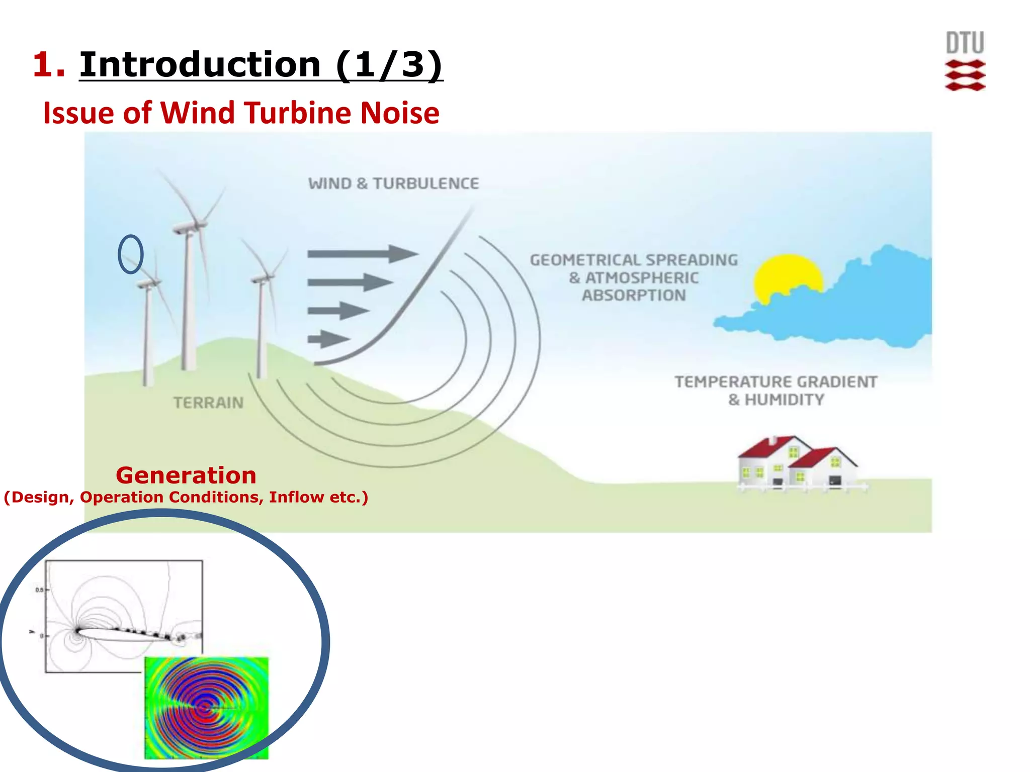
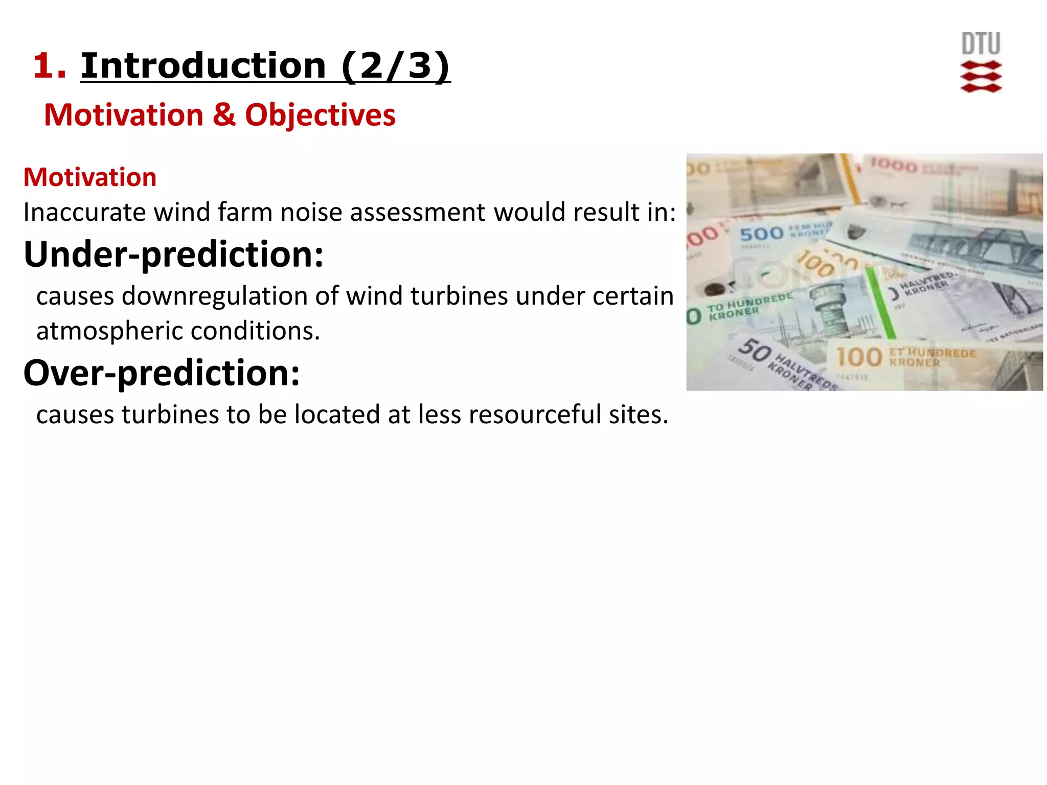
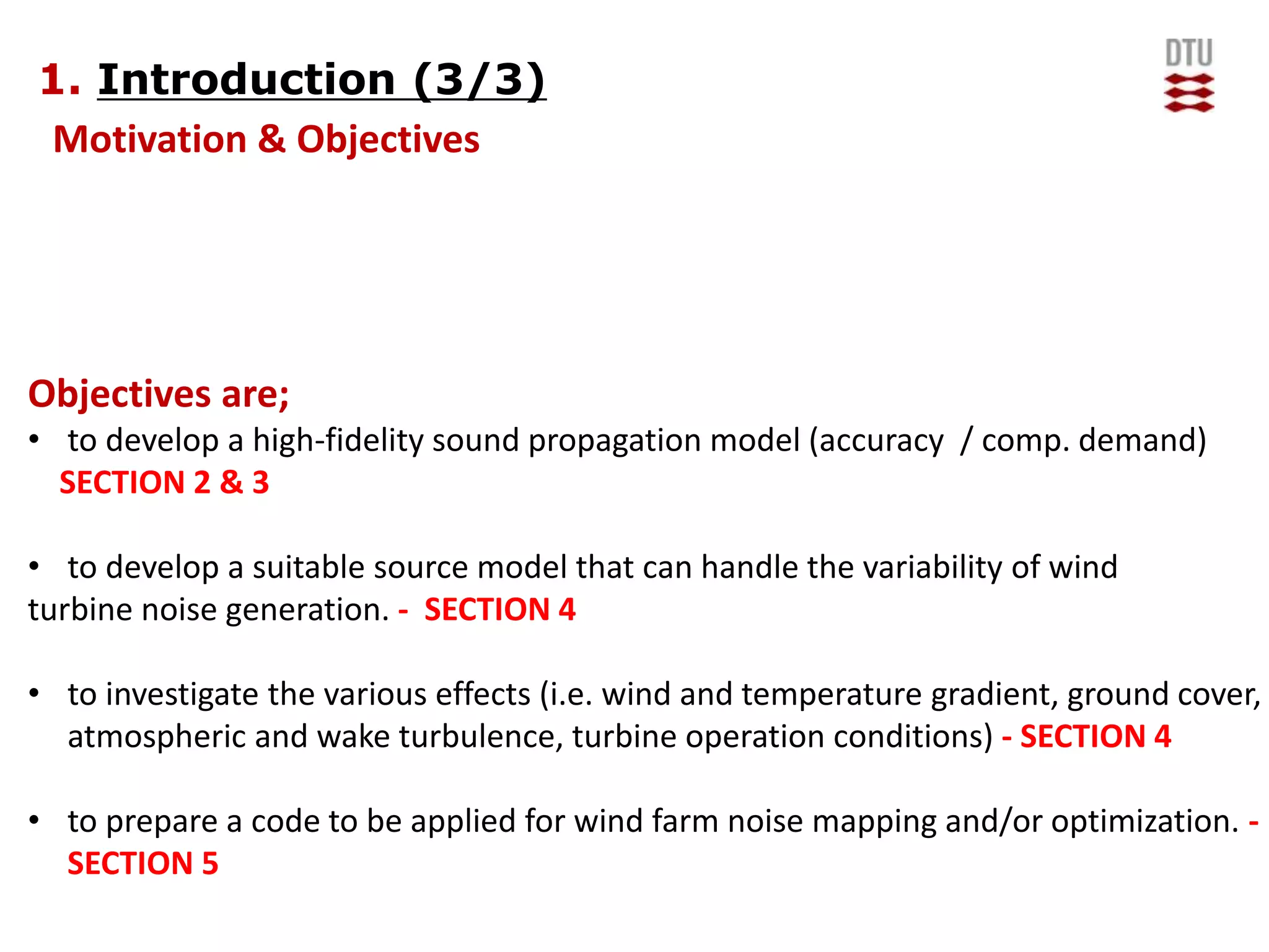
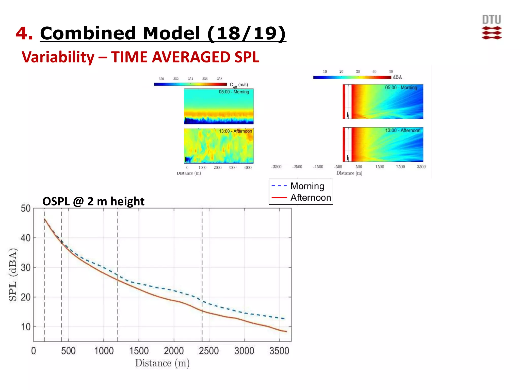
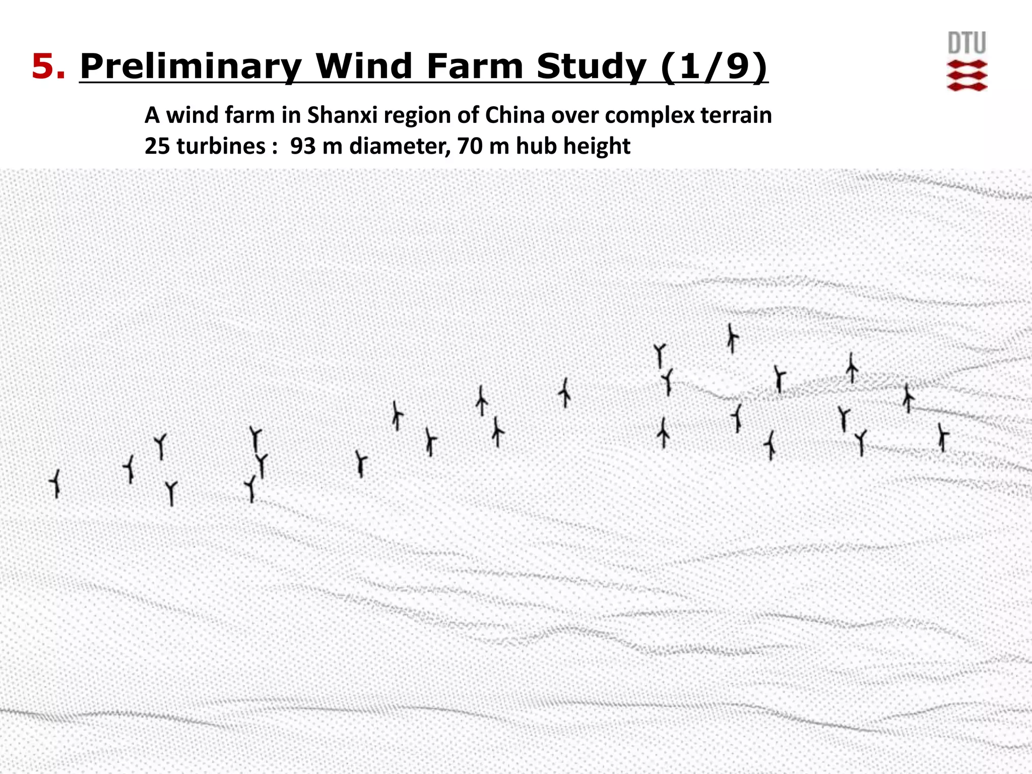
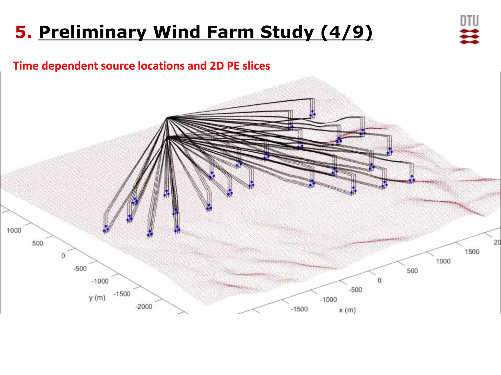
The document discusses the development of an advanced noise propagation model aimed at optimizing noise assessment for wind farms, addressing issues such as design, operational conditions, and atmospheric effects. It outlines objectives including creating a high-fidelity sound model and preparing a code for noise mapping, along with a combined model that incorporates various factors affecting noise generation and propagation. Preliminary studies on a wind farm in complex terrain further demonstrate the model's capabilities and suggest areas for future research.

1. Development of an advanced noise propagation
model for noise optimization in wind farm
Emre Barlas
Supervisors: Wen Z. Shen, Wei J. Zhu, Jens N. Sørensen
PhD Defense
DTU Wind Energy
Department of Wind Energy
Fluid Mechanics
26.01.2018
1

2. 1. Introduction & Motivation
2. Atmospheric Acoustics & Modelling
3. Sound Propagation & Wind Turbine Wake
4. Wind Turbine Noise Generation & Propagation Model
5. Preliminary Wind Farm Study
6. Conclusions & Future Work
Content

3. 1. Introduction (1/3)
Issue of Wind Turbine Noise

4. 1. Introduction (1/3)
Issue of Wind Turbine Noise
Generation
(Design, Operation Conditions, Inflow etc.)

5. 1. Introduction (1/3)
Issue of Wind Turbine Noise
Propagation
(atmospheric conditions, terrain, ground characteristics etc. )

6. 1. Introduction (1/3)
Issue of Wind Turbine Noise
Perception
(social background, age, landscape etc.

7. Motivation & Objectives
Motivation
Inaccurate wind farm noise assessment would result in:
Under-prediction:
causes downregulation of wind turbines under certain
atmospheric conditions.
Over-prediction:
causes turbines to be located at less resourceful sites.
1. Introduction (2/3)

8. Objectives are;
• to develop a high-fidelity sound propagation model (accuracy / comp. demand)
SECTION 2 & 3
• to develop a suitable source model that can handle the variability of wind
turbine noise generation. - SECTION 4
• to investigate the various effects (i.e. wind and temperature gradient, ground cover,
atmospheric and wake turbulence, turbine operation conditions) - SECTION 4
• to prepare a code to be applied for wind farm noise mapping and/or optimization. -
SECTION 5
Motivation & Objectives
1. Introduction (3/3)

9. 1. Introduction & Motivation
2. Atmospheric Acoustics & Modelling
3. Sound Propagation & Wind Turbine Wake
4. Wind Turbine Noise Generation & Propagation Model
5. Preliminary Wind Farm Study
6. Conclusions & Future Work
Content

10. 2. Atmospheric Acoustics & Modelling (1/6)

11. Engineering approach
– Ray model (very fast, limited accurate).
Accurate numerical approach: Time domain (expensive, propagation in all
directions)
– DNS, LES/CAA: compute source + propagation, based on solving Navier-
Stokes equations.
– FDTD: given source + propagation, based on solving Euler equations
Accurate numerical approach: Frequency domain (less expensive, one way
propagation)
– Parabolic equation (PE)
– Fast Field Program (FFP) (layered atmosphere and homogeneous
ground)
2. Atmospheric Acoustics & Modelling (2/6)

12. 2. Atmospheric Acoustics & Modelling (2/6)
Engineering approach
– Ray model (very fast, the least accurate).
Accurate numerical approach: Time domain (expensive, propagation in all
directions)
– DNS, LES/CAA: compute source + propagation, based on solving Navier-
Stokes equations.
– FDTD: given source + propagation, based on solving Euler equations
Accurate numerical approach: Frequency domain (less expensive, one way
propagation)
– Parabolic equation (PE)
– Fast Field Program (FFP) (layered atmosphere and homogeneous
ground)

13. Propagation Model : Parabolic Equation Method
2. Atmospheric Acoustics & Modelling (3/6)

14. Propagation Model : Parabolic Equation Method
Solve the wave equation with;
General assumptions; Implies;
• Harmonic wave - Frequency Domain
• Axisymmetric - 2D
• Far field - Long range propagation
• One way propagation - Waves that are traveling from the source to the receiver (no backscattering
• Effective Speed of Sound (optional) - Moving atmosphere is replaced by a hypothetical motionless medium
with the effective sound speed.
2. Atmospheric Acoustics & Modelling (3/6)

15. Propagation Model : Parabolic Equation Method
Solve the wave equation with;
General assumptions; Implies;
• Harmonic wave - Frequency Domain
• Axisymmetric - 2D
• Far field - Long range propagation
• One way propagation - Waves that are traveling from the source to the receiver (no backscattering
• Effective Speed of Sound (optional) - Moving atmosphere is replaced by a hypothetical motionless medium
with the effective sound speed.
OR
2. Atmospheric Acoustics & Modelling (3/6)

16. 2. Atmospheric Acoustics & Modelling (6/6)
With
turbulence
Without
turbulence
Transmission Loss for 800 Hz
Wind
direction
dB

17. 1. Introduction & Motivation
2. Atmospheric Acoustics & Modelling
3. Sound Propagation & Wind Turbine Wake
4. Wind Turbine Noise Generation & Propagation Model
5. Preliminary Wind Farm Study
6. Conclusions & Future Work
Content

18. Receiver
3. Sound Propagation & Wake (1/6)
SOFAR Channel
in the ocean
(sound fixing and ranging channel)
Noise Behind a Barrier
in the atmosphere
SPL with Non Varying Wind
SPL with Varying Wind

19. 3. Sound Propagation & Wake (2/6)
Turbine : NM 80 - Incoming Turbulence Int. : 3%
Snapshot of the flow field obtained from unsteady simulations
Time Averaged Wind Profile

20. 3. Sound Propagation & Wake (3/6)

21. 3. Sound Propagation & Wake
skipped

22. 1. Introduction & Motivation
2. Atmospheric Acoustics & Modelling
3. Sound Propagation & Wind Turbine Wake
4. Wind Turbine Noise Generation & Propagation Model
5. Preliminary Wind Farm Study
6. Conclusions & Future Work
Content

23. 4. Combined Model (1/19)
Generation
(Design, Operation Conditions,
Inflow etc.)
Propagation
(atmospheric conditions, terrain, ground
characteristics etc. )

24. COMBINED MODEL OVERVIEW
UNSTEADY FLOW MODEL
(Large Eddy Simulation)
Aeroelastics tool (FAST v8)
+
Semi Empirical Airfoil Noise (BPM)
Propagation
(Parabolic Equation)
1
2
3

26. 4. Combined Model (3/19)
Source : Aeroelastics + Aeroacoustics
Turbulent Boundary Layer
Trailing Edge noise
Separation-Stall noise
Turbulent Inflow Noise

27. Store the highest SPL contributor airfoil location
along each blade
(freq, blade, receiver, time)
4. Combined Model (4/19)
Source : Aeroelastics + Aeroacoustics
Source Locations
For 2 frequencies

28. Run PE (freq,blade,receiver,time)
4. Combined Model (5/19)

29. 4. Combined Model (6/19)

30. Source Only Simulations
OSPL @ 2 m receiver height 20-1000 Hz
Interpolated in between receivers
Variability is caused by
• Blade Movement
• Angle of attack and TI
change due to turbulent
atmosphere
Lacking propagation physics
• Atmosphere (refraction)
• Ground (reflection)
4. Combined Model (8/19)

31. Coupled Simulations
OSPL @ 2 m receiver height 20-1000 Hz
Interpolated in between receivers
Z0 – Roughness Value : 0.6 m
Neutrally stratified atmosphere
Grassland
4. Combined Model (9/19)

32. Amplitude Modulation
4. Combined Model (10/19)

33. Amplitude Modulation
Source Only Simulations
Wind Direction
High AM at crosswind
4. Combined Model (10/19)
TOP VIEW

34. Wind Direction
High AM at crosswind &
Downwind & Upwind
Amplitude Modulation
Coupled Simulations
4. Combined Model (11/19)
TOP VIEW

35. Amplitude Modulation
Coupled Simulations
Wind Direction
High AM at crosswind &
Downwind & Upwind
4. Combined Model (12/19)
TOP VIEW

36. LES Flow Field Output
• Horizontal slice at hub height
• Vertical Slice at the rotor
4. Combined Model (13/19)

37. Unsteady nature of
wake + unsteady
nature of the
source results in
‘’unexpected’’ far
field modulation
Flow @ Hub height With WakeOSPL @ 2m height With Wake
Flow @ Hub height Without WakeOSPL @ 2m height Without Wake

38. Amplitude Modulation - Coupled Simulations Wake Effect
4. Combined Model (15/19)

39. 4. Combined Model (16/19)
Variability
Flow variability
During a day for the
same hub height
wind speed

40. 4. Combined Model (17/19)
Variability - SNAPSHOT
FLOW SOUND PRESSURE LEVELS

41. 4. Combined Model (18/19)
Variability – TIME AVERAGED SPL
OSPL @ 2 m height

42. 4. Combined Model (18/19)
Variability – TIME AVERAGED SPL
OSPL @ 2 m height Spectra at different distances

43. 4. Combined Model (19/19)
Variability - AMPLITUDE MODULATION
Ampl. Modul.

44. 5. Preliminary Wind Farm Study (1/9)
A wind farm in Shanxi region of China over complex terrain
25 turbines : 93 m diameter, 70 m hub height

45. 5. Preliminary Wind Farm Study (2/9)
RANS Flow Field - EllipSys3D
Stream-wise velocity
different 2d slices
Wind Direction
Wind Direction

46. 5. Preliminary Wind Farm Study (4/9)
Time dependent source locations and 2D PE slices

47. 5. Preliminary Wind Farm Study (4/9)
Time dependent source locations and 2D PE slices

48. 5. Preliminary Wind Farm Study (5/9)
Receiver distribution around the wind farm

49. 5. Preliminary Wind Farm Study (6/9)
OSPL around the wind farm

50. 5. Preliminary Wind Farm Study (7/9)
Parameter study with 4 cases.
CASE NUMBER TERRAIN WIND
1 FLAT NO WIND
(homogenous atmosphere)
2 FLAT LOG WIND
3 COMPLEX LOG WIND
4 COMPLEX RANS WIND

51. 5. Preliminary Wind Farm Study (8/9)

52. 5. Preliminary Wind Farm Study (9/9)
Difference between flat
and complex terrain
Difference between log wind
and RANS flow (both complex terrain)

53. 6. Conclusions and Future Work
Objectives were;
• to develop a high-fidelity sound propagation model (accuracy / comp. demand)
• to develop a suitable source model that can handle the variability of wind
turbine noise generation.
• to investigate the various effects (i.e. wind and temperature gradient, ground cover, atmospheric
and wake turbulence, turbine operation conditions)
• to prepare a code to be applied for wind farm noise mapping and/or optimization.
53

54. 6. Conclusions and Future Work
Objectives were;
• to develop a high-fidelity sound propagation model (accuracy / comp. demand)
Fortran/MPI implementation for Parabolic Wave Equation (vector or scalar PE).
• to develop a suitable source model that can handle the variability of wind
turbine noise generation.
• to investigate the various effects (i.e. wind and temperature gradient, ground cover, atmospheric
and wake turbulence, turbine operation conditions)
• to prepare a code to be applied for wind farm noise mapping and/or optimization.
54

55. 6. Conclusions and Future Work
Objectives were;
• to develop a high-fidelity sound propagation model (accuracy / comp. demand)
Fortran/MPI implementation for Parabolic Wave Equation (vector or scalar PE).
• to develop a suitable source model that can handle the variability of wind
turbine noise generation.
Point sources represented within PE model, in which the source power levels are obtained from airfoil
aeroacoustics combined with aeroelastic simulations and high fidelity solvers LES.
• to investigate the various effects (i.e. wind and temperature gradient, ground cover, atmospheric
and wake turbulence, turbine operation conditions)
• to prepare a code to be applied for wind farm noise mapping and/or optimization.
55

56. 6. Conclusions and Future Work
Objectives were;
• to develop a high-fidelity sound propagation model (accuracy / comp. demand)
Fortran/MPI implementation for Parabolic Wave Equation (vector or scalar PE).
• to develop a suitable source model that can handle the variability of wind
turbine noise generation.
Point sources represented within PE model, in which the source power levels are obtained from airfoil
aeroacoustics combined with aeroelastic simulations and high fidelity solvers LES.
• to investigate the various effects (i.e. wind and temperature gradient, ground cover, atmospheric
and wake turbulence, turbine operation conditions)
Day & Night / Ground & Terrain effects (next slide).
• to prepare a code to be applied for wind farm noise mapping and/or optimization.
56

57. 6. Conclusions and Future Work
Objectives were;
• to develop a high-fidelity sound propagation model (accuracy / comp. demand)
Fortran/MPI implementation for Parabolic Wave Equation (vector or scalar PE).
• to develop a suitable source model that can handle the variability of wind
turbine noise generation.
Point sources represented within PE model, in which the source power levels are obtained from airfoil
aeroacoustics combined with aeroelastic simulations and high fidelity solvers LES.
• to investigate the various effects (i.e. wind and temperature gradient, ground cover, atmospheric
and wake turbulence, turbine operation conditions)
Day & Night / Ground & Terrain effects (next slide).
• to prepare a code to be applied for wind farm noise mapping and/or optimization.
Wind Farm Study 57

58. 6. Conclusions and Future Work
• Time Averaged SPL can be captured within reasonable accuracy via
moving 2D source + mean flow
• Near field daytime levels are higher than night time levels due to enhanced
turbulence under convective conditions.
• The atmospheric conditions affect propagation significantly and in the far
field levels at night time are higher than daytime. (contrary to near field)
• Wake is an important factor for downwind propagation.
Wake deficit entrapment
• Unsteady Wake + Unsteady Sources lead to enhanced far field AM.
58

59. 6. Conclusions and Future Work
Future Work
• Unsteady Wind Farm Noise
• Wind Farm Control
• Further validation
59