This document is a thesis submitted by Caleb J. Waugh to the Department of Nuclear Science and Engineering at MIT in partial fulfillment of the requirements for a Master of Science degree. The thesis describes an improved method for measuring the absolute deuterium-deuterium (DD) neutron yield from inertial confinement fusion experiments and calibrating neutron time-of-flight detectors. The method directly calibrates neutron time-of-flight detectors in situ using CR-39 range filter proton detectors, which provide a more accurate calibration than previous cross-calibration methods. Data from exploding pusher campaigns on the OMEGA laser facility suggest that the existing OMEGA neutron time-of-flight calibration is low by 9.0


![9
List of Figures
Figure 1. First ionization energies of the elements (energy required to free one electron).18
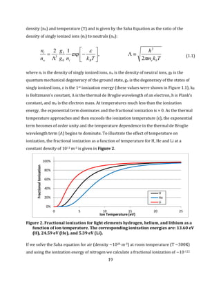
Figure 2. Fractional ionization for light elements hydrogen, helium, and lithium as a
function of ion temperature. The corresponding ionization energies are: 13.60 eV (H),
24.59 eV (He), and 5.39 eV (Li)..................................................................................................................... 19
Figure 3. The Cat's Eye nebula as seen from the Hubble telescope................................................ 20
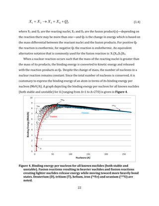
Figure 4. Binding energy per nucleon for all known nuclides (both stable and unstable).
Fusion reactions resulting in heavier nuclides and fission reactions creating lighter nuclides
release energy while moving toward more heavily bond states. Deuterium (D), tritium (T),
helium, iron (56Fe) and uranium (235U) are noted. ............................................................................... 22
Figure 5. Image depicting the standard fusion problem [3]. A nuclei with energy ε is
incident on a second nuclei. As the two nuclei approach the Coulomb repulsive force acts to
push the two particles apart. Under classical mechanics, if the relative energy (center of
mass energy) of the two particles is less than Vb the two particles will not fuse. However,
under quantum mechanics there is a finite probability of the particles tunneling through
the Coulomb barrier even though ε is lower than the Vb. .................................................................. 24
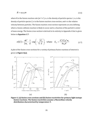
Figure 6. (a) fusion cross sections and (b) fusion reactivities for primary light isotope
fusion reactions. The fusion reactivities assume a Maxwellian velocity distribution
characterized by temperature T................................................................................................................... 26
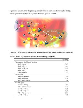
Figure 7. The first three steps in the proton-proton (pp) fusion chain resulting in 4He........ 28
Figure 8. Natural and man-made regimes in high-energy-density physics. ............................... 29
Figure 9. Areial views taken of the Nevada test site. Both images depict craters left from
underground tests. ............................................................................................................................................ 34
Figure 10. The Titan supercomputer at Oak Ridge National Laboratory..................................... 36
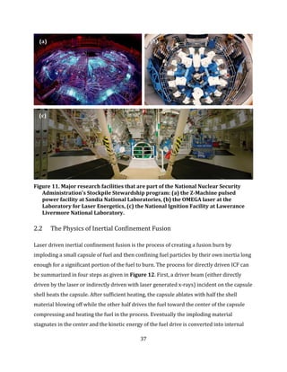
Figure 11. Major research facilities that are part of the National Nuclear Security
Administration's Stockpile Stewardship program: (a) the Z-Machine pulsed power facility
at Sandia National Laboratories, (b) the OMEGA laser at the Laboratory for Laser
Energetics, (c) the National Ignition Facility at Lawerance Livermore National Laboratory.
................................................................................................................................................................................... 37](https://image.slidesharecdn.com/2ef4ba81-4ba4-4126-9f57-f636cceccd99-160618062518/85/WaughThesis-v2-2-9-320.jpg)
![10
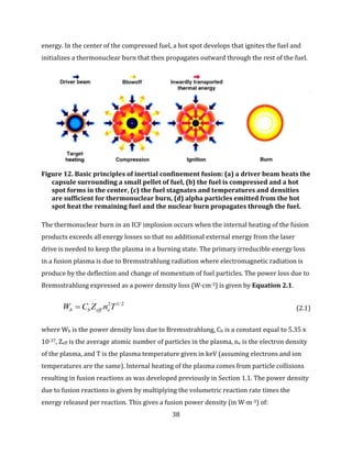
Figure 12. Basic principles of inertial confinement fusion: (a) a driver beam heats the
capsule surrounding a small pellet of fuel, (b) the fuel is compressed and a hot spot forms
in the center, (c) the fuel stagnates and temperatures and densities are sufficient for
thermonuclear burn, (d) alpha particles emitted from the hot spot heat the remaining fuel
and the nuclear burn propagates through the fuel............................................................................... 38
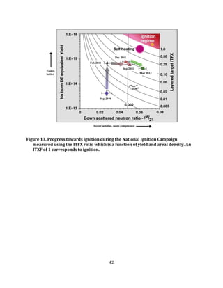
Figure 13. Progress towards ignition during the National Ignition Campaign measured
using the ITFX ratio which is a function of yield and areal density. An ITXF of 1 corresponds
to ignition.............................................................................................................................................................. 42
Figure 14. A sample nTOF response with the raw single passed through an inverting
amplifier and fit using the method outlined in [27, 28]. An absolute neutron yield for DD
and DT neutrons is obtained by time integrating the signal (SnTOF) and then multiplying by a
detector-specific calibration coefficient (CnTOF). (Figure as given in [29]).................................. 44
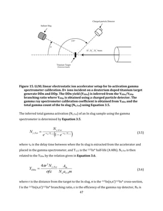
Figure 15. LLNL linear electrostatic ion accelerator setup for In-activation gamma
spectrometer calibration. D+ ions incident on a deuterium doped titanium target generate
DDn and DDp. The DDn yield (YDDn) is inferred from the YDDn/YDDp branching ratio where
YDDp is obtained using a charged particle detector. The gamma ray spectrometer calibration
coefficient is obtained from YDDn and the total gamma count of the In slug (Nγ,Tot) using
Equation 3.5......................................................................................................................................................... 47
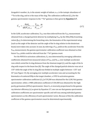
Figure 16. Flowchart outlining the series of cross-calibrations leading to the current
OMEGA nTOF calibration coefficient. Values in ◊ represent fundamental diagnostic
measurements, values in ⧠ represent calculations, and values in ○ represent fundamental
calculated quantities. (a) The gamma spectrometer calibration coefficient (Cγ:NOVA) was
obtained from the observed gamma count (Nγ,Cnt) and DD proton yield (YDDp) on a
Cockcroft-Walton accelerator. (b) The NOVA 2m nTOF calibration coefficient (CnTOF:NOVA)
was obtained from the NOVA In-activation system over a series of shots on NOVA. NOVA
10m nTOF was then cross calibrated to NOVA 2m nTOF. (c) The OMEGA gamma
spectrometer calibration coefficient (Cγ:NOVA) was obtained through cross-calibration to the
NOVA 10m nTOF. Finally, (d) OMEGA nTOF calibration coefficients CnTOF:OMEGA were
obtained through cross calibration to the OMEGA In-activation system..................................... 52](https://image.slidesharecdn.com/2ef4ba81-4ba4-4126-9f57-f636cceccd99-160618062518/85/WaughThesis-v2-2-10-320.jpg)
![11
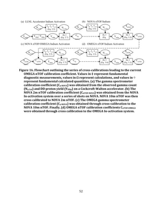
Figure 17. Flowchart outlining the steps for a method to obtain detector-specific nTOF
calibration coefficients in situ during ICF implosions using CR-39 nuclear track detector
range filter (RF) modules. The values in ◊ represent fundamental diagnostic
measurements, values in ⧠ represent calculations, and values in ○ represent fundamental
calculated quantities......................................................................................................................................... 53
Figure 18. (a) Campaign A, (b) and Campaign B exploding pusher shot campaigns on
OMEGA used to obtain an absolute yield calibration coefficient for 3m nTOF.......................... 54
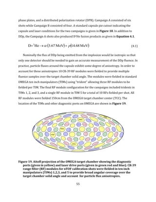
Figure 19. Aitoff projection of the OMEGA target chamber showing the diagnostic ports
(given in yellow) and laser drive ports (given in green red and blue). CR-39 range filter
(RF) modules for nTOF calibration shots were fielded in ten inch manipulators (TIMs)
1,2,3, and 5 to provide broad angular coverage over the target chamber solid angle and
account for particle flux anisotropies. ...................................................................................................... 55
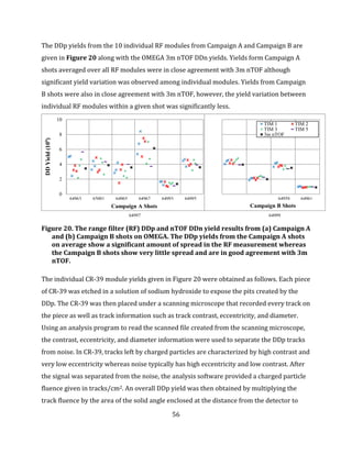
Figure 20. The range filter (RF) DDp and nTOF DDn yield results from (a) Campaign A and
(b) Campaign B shots on OMEGA. The DDp yields from the Campaign A shots on average
show a significant amount of spread in the RF measurement whereas the Campaign B shots
show very little spread and are in good agreement with 3m nTOF............................................... 56
Figure 21. The simulated capsule radius and areal density are given for shot 64999 as a
funciton of time (where t = 0 corresponds to the beginning of the laser pulse)....................... 59
Figure 22. Measured and modeled values of proton track diameter in CR-39 as a function of
incident proton energy (MeV). As given in Seguin et al. [31]. .......................................................... 60
Figure 23. CPS2 measured energy spectrums for (a) shot 64967 (Campaign A—D3He) and
(b) shot 64961 (Campaign B—DD)............................................................................................................. 61
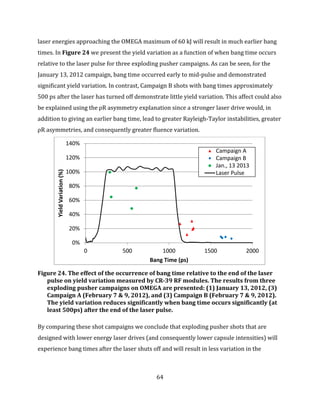
Figure 24. The effect of the occurrence of bang time relative to the end of the laser pulse on
yield variation measured by CR-39 RF modules. The results from three exploding pusher
campaigns on OMEGA are presented: (1) January 13, 2012, (3) Campaign A (February 7 &
9, 2012), and (3) Campaign B (February 7 & 9, 2012). The yield variation reduces
significantly when bang time occurs significantly (at least 500ps) after the end of the laser
pulse........................................................................................................................................................................ 64
Figure 25. The YDDn/YDDp branching ratio is given by the ratio of the parameterized reaction
rates obtained from Bosch and Hale for DDn and DDp. This ratio as a function of ion](https://image.slidesharecdn.com/2ef4ba81-4ba4-4126-9f57-f636cceccd99-160618062518/85/WaughThesis-v2-2-11-320.jpg)
![12
temperature is given by the black line. The inferred branching ratios for the OMEGA
Campaign A and Campaign B shots are obtained using the fuel burn-averaged ion
temperatures from nTOF and plotted on the black line. The error bars given for each shot in
Campaign A and Campaign B indicate the measured error in the nTOF ion temperature
measurement (x-axis) and the inferred error in the branching ratio (y-axix). ......................... 67
Figure 26. The expected value of the average of the RFn/nTOF DDn yield ratio
(E[<YRFn/YnTOF>]) with the associated 95% confidence interval obtained from the error
analysis for the OMEGA Campaign A and Campaign B shots............................................................ 71
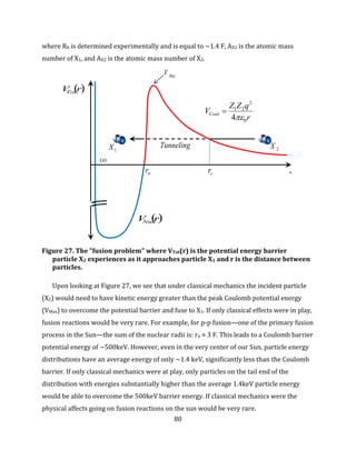
Figure 27. The "fusion problem" where VTot(r) is the potential energy barrier particle X2
experiences as it approaches particle X1 and r is the distance between particles. .................. 80
Figure 28. The wave-function solution to the Schrodinger equation for the fusion problem.
................................................................................................................................................................................... 87
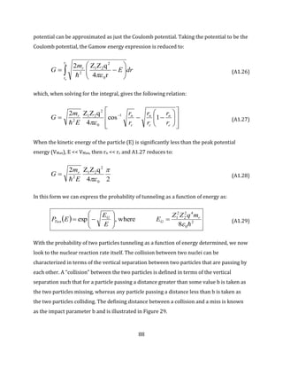
Figure 29. Impact parameter b, and cross section of nuclear collision......................................... 89
Figure 30. Fusion collisions with a density of target particles......................................................... 90
Figure 31. Linear Electrostatic Ion Accelerator (LEIA)....................................................................... 92
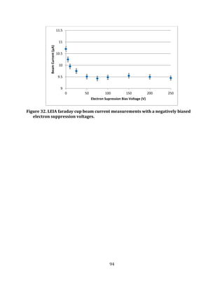
Figure 32. LEIA faraday cup beam current measurements with a negatively biased electron
suppression voltages........................................................................................................................................ 94
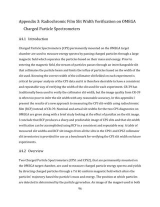
Figure 33. Magnet used for both CPS1 and CPS2 with particles entering from the "target"
end and being deflected based on particle energy (Figure courtesy of LLE standard
operating procedure D-ES-P-092)............................................................................................................... 97
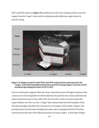
Figure 34. (a) CPS data cartridge assembly showing the baseplate, slit finger, CR-39 nuclear
track detector fingers, and slit-width x-ray finger. (b) Data cartridge assembly being
mounted over the magnet in CPS1 (Both figures courtesy of LLE standard operating
procedure D-ES-P-092). .................................................................................................................................. 98
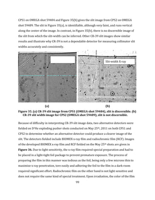
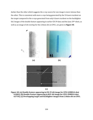
Figure 35. (a) CR-39 slit image from CPS1 (OMEGA shot 59484), slit is discernible. (b) CR-
39 slit width image for CPS2 (OMEGA shot 59489), slit is not discernible................................. 99
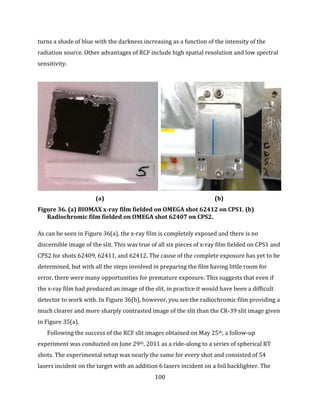
Figure 36. (a) BIOMAX x-ray film fielded on OMEGA shot 62412 on CPS1. (b) Radiochromic
film fielded on OMEGA shot 62407 on CPS2. ........................................................................................100
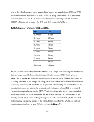
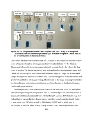
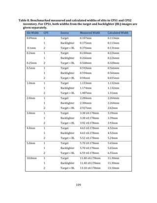
Figure 37. Inventory of CPS1 slits include nominal widths of 0.09mm, 0.2mm, 0.5mm,
1.0mm, 2.0mm, 3.0mm, 4.0mm, 5.0mm, and 10.0mm. .....................................................................102](https://image.slidesharecdn.com/2ef4ba81-4ba4-4126-9f57-f636cceccd99-160618062518/85/WaughThesis-v2-2-12-320.jpg)


![17
1 Introduction
“…if both observation and conceptualization,
fact and assimilation to theory, are inseparably linked in discovery,
then discover is a process and must take time…”
—Thomas Kuhn [1]—
Understanding of the cosmos and the nature of terrestrial substance has a long tradition
dating back to the very first of the natural philosophers who sought to apply the tools of
reason to overthrow the confines of mythological explanations of the universe and
establish complete and consistent arguments for the nature of the phenomena they
observed. Of the first in the tradition, Thales of Miletus circa 600 B.C. claimed all substance
was made of water. Anaximenes circa 550 B.C. claimed all substance was air. Later,
Heraclitus circa 500 B.C. claimed all was fire, while Empedocles synthesizing all preceding
views, and adding a fourth, claimed all substance was air, fire, water, or earth. In 350 B.C.
Aristotle accepted Empedocles categorization of the earthly substances and added a fifth,
aether, the perfect and unchanging material of the celestial regions and heavenly bodies
that was otherworldly compared to the terrestrial elements which are subject to change,
rot and decay. This view of the heavens as a place of unchanging perfection lasted for 2000
years until Galileo, while staring through the lens of his telescope in Padua in the 16th
century, observed mountains, craters, and other imperfections on the surface of the moon,
suggesting that what was once regarded in reverence as perfect, unchanging, and divine,
was strikingly more similar to the terrestrial elements then had ever previously been
thought.
In our day the Aristotelian paradigm for terrestrial substance has long been replaced,
but at the same time this ancient categorization of substance is strikingly similar to what
we now view as the four states of matter: solids, liquids, gases, and plasma. Solids are
characterized by strong binding between particles with low kinetic energy. As the kinetic
energy of the particles increases, the solid experiences a phase transition to liquid where
the particles are still bound together although the bonds are much weaker. In water at](https://image.slidesharecdn.com/2ef4ba81-4ba4-4126-9f57-f636cceccd99-160618062518/85/WaughThesis-v2-2-17-320.jpg)

![21
the universe. Atoms, as Democritus claimed, were infinite in number, could be different in
kind, size, and shape, and were separated by empty space or void. The processes
responsible for creating daughter atoms of different kind, size, and shape, from parent
atoms of smaller Z only occur when matter is in the plasma state through nuclear fusion
reactions. Additionally, nuclear fission and radioactive decay (e.g. alpha, beta, and gamma
decay) produce daughter atoms from parent atoms of higher Z. The process responsible for
creating new atomic nuclei from pre-existing nucleons with smaller Z through nuclear
fusion is called nucleosynthesis. We now turn the problem of how atoms are formed and
the nuclear reactions that lead to their formation.
In Albert Einstein’s paradigm-shattering paper “On the Electrodynamics of Moving
Bodies” we learn that the rest mass of a particle can be expressed as an energy equivalence
that is given by the famous equation E=mc2 [2]. One result of this relationship is that any
change in the rest mass of an atom leads to a change in its kinetic energy as given in
Equation 1.2:
2
cmE (1.2)
where ΔE is in joules, Δm is in kilograms, and c is in meters per second. In nuclei, this mass
differential contributes to the binding energy, EB , that is responsible for binding the
nuclear protons and neutrons together. The binding energy is expressed in terms of the
mass differential between the total mass of the individual protons, neutrons and electrons,
and the actual mass of the atom as a whole. The binding energy relationship is given in
Equation 1.3:
2
cmZXmmNmZE e
A
npB (1.3)
where Z is the number of protons and electrons, N is the number of neutrons, mp is the
proton mass, mn is the neutron mass, me is the electron mass, and m(AX) is the mass of
atom X with atomic mass number A. Nuclear reactions are often represented similarly to
chemical reactions with the reactants on the left side and the products on the right side of a
reaction chain. An example of this is given by Equation 1.4](https://image.slidesharecdn.com/2ef4ba81-4ba4-4126-9f57-f636cceccd99-160618062518/85/WaughThesis-v2-2-21-320.jpg)
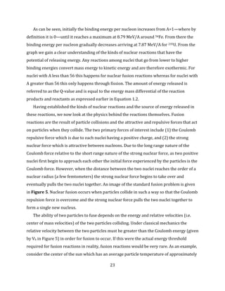
![24
1.4keV and an energy distribution that is roughly Maxwellian. Based on Figure 5, the
Coulomb barrier is estimated as being on the order of 500keV (for proton/proton and
deuterium/proton collisions). If only classical mechanics were at play only particles with
energies substantially higher than the average 1.4keV particle energy in a Maxwellian
energy distribution would be able to overcome the 500keV barrier energy. If only classical
mechanics were considered fusion reactions on the sun would be very rare.
Figure 5. Image depicting the standard fusion problem [3]. A nuclei with energy ε is
incident on a second nuclei. As the two nuclei approach the Coulomb repulsive
force acts to push the two particles apart. Under classical mechanics, if the
relative energy (center of mass energy) of the two particles is less than Vb the two
particles will not fuse. However, under quantum mechanics there is a finite
probability of the particles tunneling through the Coulomb barrier even though ε
is lower than the Vb.
However, classical mechanics are not the only phenomena when it comes to fusion
reactions. Due to quantum effects where particles exhibit wave-like properties and are
represented mathematically as waves, there exists a finite probability that one particle
colliding with another particle will “tunnel” through the potential barrier (Vb) even if the
relative energy between the particles (ε) is less than Vb. The derivation of this probability is
somewhat involved and is provided in detail in Appendix A. The resulting probability of](https://image.slidesharecdn.com/2ef4ba81-4ba4-4126-9f57-f636cceccd99-160618062518/85/WaughThesis-v2-2-24-320.jpg)
![25
one particle tunneling through the potential barrier to a second particle was originally
derived by Gamow [4] and is given here as:
2
0
42
2
2
1
8
where,exp
r
G
G
Tun
mqZZ
E
E
E
EP
(1.5)
where E is the center of mass energy of the particles, EG is the Gamow energy, mr is the
reduced mass of the two particles (mr =(m1+m2)/(m1*m2)), m1 is the mass of particle 1, m2
is the mass of particle 2, ħ is the reduced Plank’s constant, Z1 is the atomic number of
particle 1, Z2 is the atomic number of particle 2, q is the charge of an electron, and ε0 is the
permittivity of free space.
When looking at the tunneling probability given by Equation 1.5 a few things stand out.
The threshold energy required to achieve a high probability of tunneling is highly affected
by the Gamow energy (EG). The higher the Gamow energy, the higher the center of mass
energy between the particles must be for tunneling to occur. The Gamow energy itself is
mainly dependent on the charge and mass of the colliding particles. The larger the atomic
number, the greater the nuclear charge, the greater the Coulomb repulsion force between
the particles, and the lower the probability the particles will tunnel. Even for the smallest of
Coulomb repulsion force between particles, the center of mass energy required for even a
small probability of tunneling can be large when compared to the ionization energy. As an
example, evaluating Equation 1.4 for a collision between deuterium and tritium and for a
tunneling probability of 10%, the energy required is on the order of 220keV. Since the
ionization energy for hydrogen is only 13.59eV we see that fusion reactions can only occur
when matter is very hot and in an ionized state.
We have now looked at the problem of fusion reactions for individual colliding
particles. In most applications of interest, instead of looking at single particle interactions
we are dealing with systems consisting of many particle collisions. For these situations we
can express the fusion reactions in terms of a fusion reaction rate that gives the number of
fusion collisions in a set volume over a given period of time. The reaction rate for particles
colliding at a set energy is derived in Appendix A and is given as:](https://image.slidesharecdn.com/2ef4ba81-4ba4-4126-9f57-f636cceccd99-160618062518/85/WaughThesis-v2-2-25-320.jpg)

![29
1.2 High Energy Density Physics
The interstellar environments in which many natural nuclear reactions and
nucleosynthesis occur are characterized by very high particle energies at high densities.
Physical systems in this regime with an energy density (product of density and
temperature) greater than around 105 J/cm3 are in the regime of high energy density
physics (HEDP). Many HEDP regimes of interest occur naturally in solar and gas-giant
cores, supernovae, neutron stars, and black holes. It was not, however, until the mid-1900s
that experimental facilities existed to probe environments in HEDP in a laboratory setting.
Many of the first experiments to cross into this regime used particle accelerators, similar to
the first one developed by Cockcroft and Walton, to focus and collimate particle beams on
stationary targets [5]. The advent of the laser in the 1960’s opened the possibility of using
high powered lasers to create HEDP environments in the lab[6]. Since being introduced,
high powered lasers in the terawatt and petawatt range have been developed as an
additional platform for creating HEDP environments in the lab. One of the primary
platforms for conducting HEDP research that has emerged since the 1950s is inertial
confinement fusion [7]. Many HEDP regimes of interest are given in Figure 8.
Figure 8. Natural and man-made regimes in high-energy-density physics.](https://image.slidesharecdn.com/2ef4ba81-4ba4-4126-9f57-f636cceccd99-160618062518/85/WaughThesis-v2-2-29-320.jpg)
![30
1.3 Thesis Outline
The primary focus of this thesis is to present work conducted aimed at reducing the
uncertainty in DDp and DDn yield measurements in inertial confinement fusion (ICF)
experiments on the OMEGA laser. In addition, some additional work in support of nuclear
diagnostic development conducted on behalf of the High Energy Density Physics group at
the MIT Plasma Science and Fusion Center is also given in the appendices.
In Chapter 2 a brief history and overview of the contemporary inertial confinement
fusion program with primary motivations for the research as well as a brief overview of
inertial confinement fusion physics is given. For a complete treatment on ICF physics see
Atzeni et al. [3]. Chapter 3 presents the background and history behind the DDn yield
measurement on the OMEGA laser and the many interconnected efforts that went into
establishing the current absolute yield calibration factor for the OMEGA nTOF detector
system. These efforts include a series of cross calibrations between accelerator DDp
measurements, indium activation systems on the NOVA1 laser and OMEGA, and cross
calibration between NOVA and OMEGA nTOF systems. In Chapter 4 an improved method
for measuring the DDp yield on OMEGA using CR-39 range filter (RF) modules is presented
from which the DDn yield can be inferred. The data obtained suggest a relationship
between particle flux anisotropies and bang time, where fluence variation is observed to be
significantly reduced when bang time occurs significantly after the end of the laser pulse.
The CR-39 DDn inferred yield is then compared to the existing nTOF DDn absolute yield
calibration for verification. Chapter 5 concludes with a summary of the findings and ideas
for next steps.
In Appendix A, a derivation of the fusion reaction rate from first principles is presented
as a supplement for the equations presented in Chapter 1. In Appendix B, work done to
install a Faraday Cup on the MIT Linear Electrostatic Ion Accelerator (LEIA) is presented as
well as beam current readings to determine optimal electron suppression bias source
1
A high power laser for ICF at Lawrence Livermore National Laboratory that was decommissioned in 1999.](https://image.slidesharecdn.com/2ef4ba81-4ba4-4126-9f57-f636cceccd99-160618062518/85/WaughThesis-v2-2-30-320.jpg)


![36
Figure 10. The Titan supercomputer at Oak Ridge National Laboratory.
In addition to the impressive supercomputing infrastructure that has been built in support
of the DOE NNSA Stockpile Stewardship’s program to create the capabilities to perform
“virtual” nuclear tests, major experimental facilities have been built with the goal of using
experimental data from ICF, equation of state, and materials tests, to benchmark computer
codes. The primary DOE laboratories supporting this effort are Los Alamos National
Laboratory, Lawrence Livermore National Laboratory, and Sandia National Laboratories.
Major experiments at these labs include the Z-Machine at Sandia National Laboratory
which is used for z-pinch driven inertial confinement fusion and material equation of state
experiments [8], the National Ignition Facility at Lawrence Livermore National Laboratory
which aims at achieving a thermonuclear burn using laser indirectly-driven ICF [9], and the
OMEGA laser at the Laboratory for Laser Energetics (LLE) at the University of Rochester
which acts as a small laser ICF test-bed [10]. Images of these research facilities are given in
Figure 10.
In addition to stockpile stewardship, other contemporary interests and motivations for
ICF research include energy and basic research in HEDP such as atomic physics, nuclear
physics, plasma physics, astrophysics, material science, and laser science. Many of these
additional interests are addressed through user programs at the major research facilities
where academic and government collaborators work to further understanding of basic
science. That said, stockpile stewardship remains the primary policy goal of the program,
has a dominant share of shot time at experimental facilities, and remains the justification
for the significant amount of federal funding ICF receives [11].](https://image.slidesharecdn.com/2ef4ba81-4ba4-4126-9f57-f636cceccd99-160618062518/85/WaughThesis-v2-2-36-320.jpg)
![41
as a Lawson-type criteria of the ignition requirement for ICF. In addition, the expression of
the ignition requirement in terms of the quantity ρR is particularly useful since ρR can be
physically interpreted as the plasma mass density integrated over the capsule radius or
areal density.
R
drrR
0
)( (2.10)
The areal density can be interpreted as the amount of material that an energetic particle
passes through while escaping the plasma sphere. Many diagnostics (such as neutron time-
of flight detectors [12] and the Magnetic Recoil Spectrometer [13]) have been developed to
probe ρR by measuring the energy downshift of fusion particles (neutrons and alpha’s) that
occurs when the particles pass through the plasma. In addition, the burn fraction can be
determined by measuring the absolute fusion yield of the implosion. From measurements
of the areal density (ρR), ion temperatures, and the overall fusion yield, progress towards
ignition criteria can be determined.
An alternative and more rigorous ignition criteria for ICF implosions that is currently
used to gauge progress toward thermonuclear ignition on the National Ignition Facility is
the Ignition Threshold Factor (ITFX). This Lawson-type ignition criteria is much more
rigorous than the simple derivation given above and is benchmarked to simulations to
account for implosion velocities, hot spot shape, entropy of the compressed fuel, and the
adiabat of the compressed fuel [14]. A plot depicting progress towards thermonuclear
ignition for a number of cryogenic shots as part of the National Ignition Campaign on the
National Ignition Facility is given in Figure 13. Here the layered target ITFX (curved lines
on the graph) is given as a function of the measured down scattered neutron ratio (which is
proportional to the areal density), and the DT yield. As can be seen, progress towards
ignition on the NIF has been significant during the Ignition Campaign going from an ITFX of
0.001 in September 2010 to 0.10 in March 2012.](https://image.slidesharecdn.com/2ef4ba81-4ba4-4126-9f57-f636cceccd99-160618062518/85/WaughThesis-v2-2-41-320.jpg)
![43
3 Previous DDn Yield Measurements and nTOF Calibration Methods
As mentioned above, in addition to areal density, the fuel burn fraction is also a key
measurement in determining the performance of an ICF implosion and this is determined
from measurements of the absolute fusion yield. Accurate absolute yield measurements are
therefore vital to determining ICF capsule performance and overall progress toward the
ignition criteria. As can be seen from Table 1, many fusion reactions of interest from
controlled fusion experiments result in charged particles such as protons, tritons, 3He and
alphas but also produce neutrons. Neutron time-of-flight (nTOF) current-mode detectors
fielded on large inertial confinement fusion (ICF) facilities, such as OMEGA [10], the
National Ignition Facility [9], and which will be fielded on Laser Megajoule (LMJ) upon
completion [15, 16], are principle diagnostics that regularly measure key properties of
neutrons produced from ICF implosions. Time-of flight refers to the time it takes neutrons
to travel from the target chamber center to the nTOF detector and is can be used to infer
particle energies and the overall neutron energy spectrum. On ICF facilities implosion
neutrons are generally generated from the primary fusion reactions of deuterium (DD), or
a deuterium/tritium fuel mix (DT) as given in Equation 3.1 and Equation 3.2.
MeV0.82HeMeV2.45nDD 3
(3.1)
MeV3.52MeV14.07nTD (3.2)
The principles of nTOF operation are straightforward. Neutrons incident on a scintillator
generate photons which are then optically coupled to a photomultiplier tube (PMT) or
photo diode (PD). More recently, nTOF detectors using chemical vapor deposition (CVD)
diamonds have been developed that directly measure the neutron response without use of
a scintillator [17].
nTOF detectors are used to diagnose: (1) the absolute neutron yield by time integrating
the neutron response [18], (2) fuel burn-average ion temperatures by fitting the signal to a
response function and then using the Brysk formula [19-24], (3) the peak neutron emission
time relative to the start of the laser pulse—also commonly referred to as shot bang-time](https://image.slidesharecdn.com/2ef4ba81-4ba4-4126-9f57-f636cceccd99-160618062518/85/WaughThesis-v2-2-43-320.jpg)
![44
[25], and more recently (4) the areal density (ρR) in cryogenic DT implosions on OMEGA
and the NIF [26]. Because the neutron response is a linear function of the number of
incident neutrons as long as the detector does not saturate, measurement of the absolute
neutron yield only requires a detector-specific calibration coefficient (CnTOF [n·mV-1·ns-1])
to relate the integrated nTOF signal (SnTOF [mV·ns]) to the neutron response as given in
Equation 3.3.
nTOFnTOFn CSY (3.3)
A sample of a typical nTOF pulse is given in Figure 14. Since the detector neutron response
varies with the neutron energy, separate calibration coefficients must be obtained to
characterize the different responses for DT (14.07 MeV) and DD (0.82 MeV) neutrons.
Figure 14. A sample nTOF response with the raw single passed through an inverting
amplifier and fit using the method outlined in [27, 28]. An absolute neutron yield
for DD and DT neutrons is obtained by time integrating the signal (SnTOF) and then
multiplying by a detector-specific calibration coefficient (CnTOF). (Figure as given
in [29]).](https://image.slidesharecdn.com/2ef4ba81-4ba4-4126-9f57-f636cceccd99-160618062518/85/WaughThesis-v2-2-44-320.jpg)
![45
Historically, detector-specific nTOF calibration coefficients were obtained by either (1)
cross-calibration to a previously calibrated nTOF, or (2) cross-calibration to Copper (Cu) or
indium (In) activation samples for DT and DD neutrons respectively [30]. In the second
approach, Cu and In slugs were activated by incident neutrons from DT and DD neutrons.
After activation the resulting Cu and In radioisotopes would decay back to stable isotopes
emitting gamma rays in the process. The calibration coefficients for the gamma ray
spectrometers used to measure gammas emitted from Cu and In-activation were obtained
separately from accelerator produced DD and DT fusion products by measuring the
charged particle counts associated with those reactions. For Cu-activation, this was done
my measuring the 3.52 MeV alpha yield from the reaction given in Equation 3.2. For In-
activation, this was done by measuring the proton yield from the other DD reaction branch,
given in Equation 3.4, and then using the corresponding branching ratio to infer an
equivalent neutron yield [30].
MeV1.01MeV3.02pDD T (3.4)
In the next two chapters, a method for obtaining detector-specific DD neutron (DDn)
nTOF calibration coefficients through an in situ measurement of DD protons (DDp)
produced during OMEGA ICF implosions is presented. The method involves calibrating the
integrated nTOF neutron response (SnTOF) to DDp measurements obtained using CR-39
nuclear track range filter (RF) modules [31]. An advantage of using CR-39 is that it has
100% particle detection when operating in optimal detection regimes and does not need to
be calibrated. An equivalent DDn yield (YDDn) is inferred from the DDp RF yield (YDDp) using
the YDDn/YDDp branching ratio which at ion temperatures common in laser driven ICF
experiments is close to unity. This approach for obtaining an nTOF absolute yield
calibration has the advantage over previous calibration methods in that: (1) it reduces the
dependence on what had been a series of multiple cross-calibrations between accelerators,
In-activation systems, and other nTOF detectors, and (2) it takes advantage of the fact that
CR-39 has 100% detection efficiency. By directly calibrating the nTOF response to a DDn
inferred yield from DDp using CR-39 RF modules, the uncertainty in the calibration
coefficient can be well quantified.](https://image.slidesharecdn.com/2ef4ba81-4ba4-4126-9f57-f636cceccd99-160618062518/85/WaughThesis-v2-2-45-320.jpg)
![49
3.2 NOVA In/nTOF Cross-calibration
With calibration coefficients determined for the NaI and HPGe gamma spectrometers, the
NOVA YDDn nTOF response was later cross-calibrated to In-activation samples fielded on a
series of NOVA ICF implosions. At the time, the NOVA nTOF system consisted of four nTOF
detectors—50cm nTOF, 2m nTOF, 10m nTOF, and 20m nTOF—located at 62cm, 1.9m,
8.36m, and 18.33m from the NOVA target chamber center respectively. For the cross-
calibrations, only the 2m nTOF was directly calibrated against neutron yields obtained
from In-activation. With a time-integrated signal (SnTOF) for 10m nTOF, and YDDn
determined using In-activation, the 10m nTOF calibration coefficient CnTOF was found using
Equation 3.3. 50 cm nTOF and 10m nTOF were then cross-calibrated against 2m nTOF, and
in subsequent shots, 20m nTOF was calibrated against 10m nTOF. A summary of the NOVA
nTOF specifications and calibration information is given in Table 3.
Table 3. nTOFs comprising the NOVA nTOF system in the 1990s along with their
corresponding distance to target chamber center (TCC), the method used for
cross-calibration, and the resulting detector-specific calibration coefficient
(CnTOF).
nTOF Detector Distance to TCC Cross-calibrated to CnTOF [n·mV-1·ns-1]
50cm 0.62m 2m nTOF 1.92x10³
2m 1.92m In-activation 3.92x10⁴
10m 8.36m 2m nTOF 6.94x10⁵
20m 18.33m 10m nTOF 3.24x10⁶
3.3 OMEGA In/NOVA nTOF Cross-calibration
In 1996, methods were explored to calibrate an In-activation system using a HPGe gamma
ray spectrometer for the OMEGA 60 laser that at that time had recently been upgraded
from OMEGA 24. The initial calibration approach was similar to that used to calibrate the](https://image.slidesharecdn.com/2ef4ba81-4ba4-4126-9f57-f636cceccd99-160618062518/85/WaughThesis-v2-2-49-320.jpg)
![50
In-activation system on NOVA previously. A 2MeV Van DeGraff accelerator at SUNY
Geneseo3 resulted in a calibration coefficient for the OMEGA HPGe gamma spectrometer of
7.35 x 10⁶. However, additional accelerator runs at SUNY Geneseo performed early in 1997
resulted in a calibration coefficient of 5.92 x 10⁵, over an order of magnitude lower than the
coefficient previously obtained. To address the discrepancy, other calibration techniques
were utilized including direct calculation of the gamma spectrometer calibration coefficient
from first principles (which resulted in a coefficient of 1.7 x 10⁷), and using a multi-line
gamma source to characterize the HPGe efficiency (which resulted in a coefficient of 8.93 x
105). Overall these early attempts at calibrating the OMEGA In-activation gamma
spectrometer resulted in large discrepancies in the calibration coefficients obtained and
the associated uncertainty regarding what the actual value of the coefficient should be.
In a final attempt to resolve the calibration discrepancy, the 10m nTOF from NOVA was
ported to and fielded on OMEGA where a calibration coefficient of 2.20 x10⁶ was obtained
(3.3 times smaller than the first calibration coefficient obtained at SUNY Geneseo). As the
NOVA 10m nTOF had originally been calibrated to an In-activation system where
consistent results had been obtained over a wide range of accelerator runs and with two
different kinds of gamma spectrometers (both the In and HPGe), the final OMEGA In-
activation system In-activation gamma spectrometer calibration coefficient used was the
one obtained through the cross-calibration to the ported NOVA 10m nTOF.
3.4 OMEGA nTOF/CR-39 Neutron Verification
In 2000, CR-39 nuclear track detectors were characterized to directly measure absolute
neutron yields in DD and DT implosions on OMEGA [32]. CR-39 is regularly used to
measure charged particle yields in the low energy range (~MeV) as charged particles leave
a trail of damage in the plastic in the form of broke molecular chins and free radicals.
Through post-shot etching of CR-39 in a sodium hydroxide solution (NaOH), damage trails
are enlarged to become conical pits or tracks that are readily identified under
3
Geneseo State University of New York, 1 College Circle, Geneseo, NY 14454.](https://image.slidesharecdn.com/2ef4ba81-4ba4-4126-9f57-f636cceccd99-160618062518/85/WaughThesis-v2-2-50-320.jpg)
![51
magnification [31]. Elastic scattering of DD neutrons within the CR-39 produce recoil
protons, or oxygen or carbon nuclei that also leave identifiable damage trails on both the
front and back sides of the CR-39 detectors. If the CR-39 neutron detection efficiency—
probability that an incident neutron produces a recoil charged particle that leaves a visible
track—is known, a neutron yield can be inferred from the recoil particle count.
The CR-39 neutron detection efficiency was determined by cross-calibration to the
OMEGA In-activation system (shot 19556). Efficiencies of (1.1 ± 0.2) x 10-4 and (3.3 ± 0.3) x
10-4 were determined for the front and back sides respectively, and were in good
agreement with Monte Carlo simulations of the neutron response. Subsequent DD shots on
OMEGA showed good agreement between the In-activation DD yield and the inferred CR-39
neutron yield, however, since the CR-39 detection efficiency was benchmarked to the
OMEGA In-activation system, these experiments do not constitute an absolute calibration
but rather only provide a CR-39 neutron detection efficiency.
3.5 OMEGA In/nTOF Cross-calibration
With the HPGe gamma ray spectrometer at OMEGA calibrated to the ported NOVA 10m
nTOF, the OMEGA nTOF system was then cross-calibrated to the OMEGA In-activation
system over a series of OMEGA ICF implosions similar to the way that the NOVA nTOF
system was calibrated to the NOVA In-activation system. On OMEGA, however, the In-
activation system continued to be used as the primary YDDn diagnostic from 1996-2000
with the nTOF system being run as a backup. As has now been shown in detail, the current
OMEGA nTOF calibration coefficients are the results of extensive cross calibrations that
took place across multiple diagnostic platforms and facilities. To aid in visualizing all the
cross-calibrations that were conducted leading to the current OMEGA nTOF calibration
coefficient, a flow chart of the cross-calibrations along with references to the equations
needed to infer fundamental calculated quantities is given in Figure 16.](https://image.slidesharecdn.com/2ef4ba81-4ba4-4126-9f57-f636cceccd99-160618062518/85/WaughThesis-v2-2-51-320.jpg)
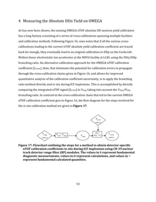
![54
4.1 High Accuracy YDDp Measurements on OMEGA using CR-39 Range Filters
As has been previously mentioned, CR-39 nuclear track detectors are widely used for
charged particle detection. As such they serve as the primary detection mechanism in a
wide array of ICF diagnostics on OMEGA and the NIF [33-44]. The CR-39 response to
protons in particular has been studied extensively and is well documented [31, 45-49].
To test the CR-39/nTOF in situ calibration method, a series of directly-driven exploding
pusher shots on OMEGA were taken where DDn yields obtained from nTOF using the
existing absolute yield calibration coefficient (CnTOF) were compared to DDn yields inferred
from DDp yields obtained from CR-39 RF modules. Exploding pushers are thin shell
capsules made of glass or plastic in which a high-density shell is heated rapidly to
temperatures on the order of a few keV and then explodes. For the experiments comprising
the study, two shot campaigns were designed to optimize both the CR-39 RF DDp and nTOF
DDn responses and reduce measurement uncertainty.
Figure 18. (a) Campaign A, (b) and Campaign B exploding pusher shot campaigns on
OMEGA used to obtain an absolute yield calibration coefficient for 3m nTOF.
For what we will henceforth refer to as Campaign A, the targets were nominally 880μm in
diameter 2.0 μm thick silicon dioxide (Si02) and were filled with 3.6 atm D2 and 7.9 atm
3He. Laser conditions included 60 beams providing a total nominal energy of 5.3 kJ. For the
second campaign, which we will refer to as Campaign B, the capsules were also nominally
880μm in diameter 2.0μm thick silicon dioxide (SiO2) filled with 9.3 atm of D2. Laser
conditions included 60 beams providing a total nominal energy of 2.5kJ. Both shot
campaigns used a 1ns square laser pulse, smoothing by spectral dispersion (SSD), SG4
9.3 atm D2
2.0 μm SiO
2
2.4 kJ
1670 ps
BT
7.9 atm
3
He
2.0 μm SiO
2
3.6 atm D2
5.2 kJ
1274 ps BT
(a) (b)](https://image.slidesharecdn.com/2ef4ba81-4ba4-4126-9f57-f636cceccd99-160618062518/85/WaughThesis-v2-2-54-320.jpg)
![57
TCC (which was 150cm). Although not given here, full details regarding the processing and
signal to noise separation in CR-39 detectors is given in Sequin et al. [31]. A full overview of
the raw data and analysis used to obtain the individual RF yield measurements is given
Figure 20 are provided in Appendix E.
Upon observing the measured yields from the shot campaigns in Figure 20—and in
particular the shots from Campaign A—ones notes the significant variation in individual RF
yield measurements within a given shot. This variation exists between the RF modules
fielded in different TIMs, but also within the RF modules fielded in a trident within a single
TIM. We now look at the source of this variation in more detail and consider whether this is
caused by: (1) instrumentation and measurement uncertainty in the individual
measurements from CR-39 RF modules, or (2) capsule implosion effects leading to an
asymmetric distribution to charged particles. What we would like to know is whether the
fluences observed really do exhibit a large degree of variance or whether the variance is
due to measurement uncertainty.
As has already been mentioned, one primary advantage of CR-39 is that when certain
criteria are met the detector exhibits 100% detection efficiency of the charged particles of
interest. To obtain 100% detection efficiency there must be 1) clear separation of charged
particle species to isolate the given particle of interest, 2) the individual particles must
have an energy that lies within the optimal CR-39 detection range, and 3) there must be
clear signal to noise separation to keep intrinsic noise in the CR-39 from being counted as
tracks.
When using CR-39 detectors to observe and isolate a single charged particle species,
range filters are commonly used to range out species not of interest and to range species of
interest into the CR-39 optimal detection energy range. For the shots comprising Campaign
A, the primary charged particles incident on the CR-39 were from the primary DD and D3He
fusion reactions and include: 3He (from the DD reaction in Equation 3.1), T (from the DD
reaction in Equation 3.4), protons (from the DD reaction in Equation 3.4), alphas (from the
D3He reaction given in Equation 4.1), and protons (also from the D3He reaction in Equation
4.1). Other lower energy ions (on the order of less than 10keV for both Campaign A and
Campaign B shots) from the SiO2 capsule and fuel were also present. For campaign B the](https://image.slidesharecdn.com/2ef4ba81-4ba4-4126-9f57-f636cceccd99-160618062518/85/WaughThesis-v2-2-57-320.jpg)
![58
primary ions were the same except for the fusion products from the D3He reaction. For
both campaigns a 25μm Al filter was placed in front of the CR-39. The thickness was chosen
so as to range out all the low energy ions from the capsule and fuel as well as all charge
particles except for the DD and D3He protons. An overview of the charged particles
generated from the primary fusion reactions from DD and D3He along with the particle
birth energy, particle range in aluminum corresponding to the birth energy, and the ranged
energy of the particle after passing through 25μm of aluminum, is given in Table 4. The
values in Table 4 assume that no ranging other than the 25μm Al range filter occurs. In
practice there is often additional ranging of particles through the fuel and capsule.
Table 4. Primary fusion product charged particles incident on CR-39 RF modules in
Campaigns A and B. Given are the source fusion reactions, the particle birth
energy, the range of the particle in aluminum corresponding to the birth energy,
and the energy of the particle after passing through the 25 μm range filter.
Ion Reaction Birth Energy (MeV) Range (um) Ranged Energy (MeV)
3He D(D,3He)n 0.82 2.70 0
Triton D(D,T)p 1.01 9.82 0
Alpha D(3He,α)p 3.67 14.10 0
Proton D(D,T)p 3.02 81.47 2.42
Proton D(3He,α)p 14.68 1222 14.50
From Table 4 we see that only DD an D3He protons are able to pass through the aluminum
range filter and all other charged particle species are stopped. energy range and are the
only charged particle species that leave observable pits in the detector.
Although only DDp are detected in the CR-39, to ensure 100% counting the entire DDp
spectrum must fall within the detectable energy range of the CR-39. In addition to range
filters which cause an energy downshift, the areal density (ρR) of the capsule and fuel in
ICF implosions can also potentially have a significant effect of ranging down the proton
energy from the original birth energy. In some studies the measured energy downshift of
primary fusion reaction protons (DDp and D3He-p) has been used to estimate the fuel ρR
[39]. If the ρR energy downshift is large enough there is a risk that the combined 25μm Al](https://image.slidesharecdn.com/2ef4ba81-4ba4-4126-9f57-f636cceccd99-160618062518/85/WaughThesis-v2-2-58-320.jpg)

![60
ranging through the 25μm of Al using SRIM, the energy incident on the CR-39 is calculated
to be ~0.7MeV.
In order for a track to be detectable on CR-39 it must fall within a detectable energy
range. The range of detectable protons can be understood by observing a plot of the proton
diameter as a function of energy as given by Seguin et al. and provided below in Figure 22.
Figure 22. Measured and modeled values of proton track diameter in CR-39 as a
function of incident proton energy (MeV). As given in Seguin et al. [31].
As can be seen, high energy protons leave small tracks on the order of 2-4μm. As the energy
reaches around 4 MeV the track diameter starts to increase significantly until it peaks
around 0.7MeV. For energies less than 0.7 MeV, the track diameter starts to get smaller as
the proton energy is reduced and approaches 0. In addition to getting smaller, the contrast
of the tracks becomes increasingly faint until they are unable to be detected by the
scanning microscope. The conclusions this figure is that for protons we should expect good
contrast of tracks and therefore full detection under the scanning microscope up to the
peak energy of 0.7MeV, after which we would gradually start losing tracks as the proton
energy goes to 0. That said, some tracks are still detectable at the lower energy levels (as](https://image.slidesharecdn.com/2ef4ba81-4ba4-4126-9f57-f636cceccd99-160618062518/85/WaughThesis-v2-2-60-320.jpg)

![63
In many ICF implosions, Rayleigh-Taylor instabilities created on the capsule surface
during compression result in areal density asymmetries. For charged particles passing
through, we would expect greater angular particle deflection in the higher density areas
than the lower density area. If the mode of these asymmetries were high enough it could
lead to the kind of anisotropic particle flux distribution observed in the data in Figure 20.
Another effect that has been observed is the presence of large electromagnetic fields that
are generated around the target as the laser ablates the capsule. These fields have been
observed in proton radiographs published by Rygg et al. in Science [33]. While the fields
have no effect on neutrons, the electromagnetic fields generated are strong enough to
deflect charged particles and could lead to an anisotropic flux of particles over the target
chamber solid angle.
4.2 Relation Between Particle Flux Anisotropies and Bang Time
As can be seen in Figure 22, individual Campaign A shots exhibit significantly more yield
variation between individual RF modules than the shots in Campaign B. As has been shown,
the variation between the individual RF module fluence measurements is not due to
measurement error: CR-39 has 100% detection efficiency and on all shots the number of
tracks counted per area analyzed varied between 25,000 and 85,000 tracks so that
counting errors were less than 1%. Consequently the variation is essentially entirely
contributed to particle flux anisotropies which currently we attribute to either ρR
asymmetries or electromagnetic fields generated around the capsule during implosion. For
the electromagnetic field explanation, these fields have been found to be strongest during
the laser pulse while the laser is incident on the capsule. In addition a circuit model of the
capsule from which electromagnetic fields can be inferred was recently presented in N.
Sinenian’s PhD thesis that also predicts significant reduction in fields shortly after the laser
has turned off [50]. Shots that are designed so that the laser is not incident on the capsule
when bang time occurs will have weaker electromagnetic fields during bang time and will
result in less yield variation. The most significant parameter that affects when bang time
occurs within the laser pulse is the laser drive energy and subsequently the capsule laser
intensity. On OMEGA, laser energies of a few kilo-joules will result in late bang times while](https://image.slidesharecdn.com/2ef4ba81-4ba4-4126-9f57-f636cceccd99-160618062518/85/WaughThesis-v2-2-63-320.jpg)
![65
individual CR-39 RF module yield measurements, hence reducing the uncertainty in the
overall yield measurement.
The trend in yield variation as a function of bang time depicted in Figure 24 can also be
used to evaluate the two explanations presented earlier regarding the cause of the
observed particle flux anisotropies. The two explanations given were that the yield
variation could be explained by 1) areal density asymmetries and 2) electromagnetic field
effects that are present during capsule implosions. For the January 13 shots that exhibited
high yield variation and early bang time the capsules were driven with a 30 kJ 1ns square
pulse. As shown before, Campaign A shots were driven with a 5.2 kJ 1ns square pulse and
Campaign B shots were driven with a 2.4 kJ 1 ns square pulse. The trend we see in Figure
24 then shows an increase in yield variation with higher laser intensity and a decrease in
yield variation with lower laser intensity. However, in Lindl et al. [51] equation 46 an
increase in laser intensity is shown to cause an increase in ablation velocity (i.e. the
velocity with which the ablation front moves through the shell), and an increase in ablation
velocity is shown to reduce the growth of Rayleigh-Taylor instabilities which would result
in less ρR assymetires. Based on the theory presented by Lindl we would then expect lesser
Rayleigh-Taylor instabilities, less ρR asymmetries and less yield variation for the January
13 shots and greater Rayleigh-Taylor instabilities, greater ρR asymmetries and greater
yield variation in the Campaign B shots. Since Figure 24 shows the exact opposite of this
the hypothesis of particle flux anisotropies being caused by ρR asymmetries is inconsistent
with the theory presented by Lindl and the observations given in Figure 24.
In addition, we consider whether the areal density of the fuel is enough to create
significant angular deflection of DDp. From the measured mean energy of 2.663 MeV
obtained in Figure 23(a) for shot 64967 we modeled the implosion using SRIM adjusting
the plasma density until the corresponding ion energy in the simulation matched the
measured mean ion energy. This resulted in a fuel density of 0.4 g/cm3 compared to the 1.2
g/cm3 predicted by the LILAC code. The mean angular deflection associated with the 0.4
g/cm3 fuel density is calculated to be 0.41° ± 0.27°. Where the CR-39 RF modules were
fielded at 150 cm from TCC, this would result in an average lateral deflection of 3.4mm ±](https://image.slidesharecdn.com/2ef4ba81-4ba4-4126-9f57-f636cceccd99-160618062518/85/WaughThesis-v2-2-65-320.jpg)
![66
2.25 mm. This suggests that we would expect very little angular deflection due to areal
density effects.
4.3 CR-39/nTOF Yield Comparison and Calibration Coefficient Verification
To verify the existing OMEGA 3m nTOF calibration coefficient and to more accurately
quantify the calibration coefficient uncertainty, uncertainties associated with the CR-39
range filter yield measurement, the nTOF yield measurement, and the DDn/DDp branching
ratio are taken into account. Uncertainties associated with the CR-39 proton response
consist of three kinds: (1) the statistical uncertainty associated with the particle counts, (2)
uncertainty in signal to noise track separation, and (3) uncertainty in the individual RF
yield measurements due to particle flux anisotropies. As the number of tracks recorded per
RF module for both shot campaigns were between 25,000 and 85,000, counting statistics
result in uncertainties less than 1% can therefore be neglected since these are much less
than the systematic calibration errors. As mentioned previously, in the analysis software
used to analyze the CR-39 tracks, noise is separated from signal by filtering tracks based on
size, eccentricity, and contrast. Using track filtering techniques, signal and noise separation
usually results in only a few percent uncertainty in the track count. With counting and
signal to noise separation uncertainties being small the uncertainties stemming from the
particle flux anisotropies dominate. Particle flux anisotropies can be reduced by increasing
the number of CR-39 RF modules fielded to obtain a greater sample size and reduce the
variance in the average yield of the detectors, or by designing shots so that bang time
occurs significantly after the end of the laser pulse so that the yield variation is small and
fewer CR-39 RF modules are needed to average out flux anisotropy affects.
Uncertainty of the nTOF measurements consists of (1) the instrumentation uncertainty
of the nTOF neutron response, cable reflections, and intrinsic noise, and (2) the uncertainty
in the calibration coefficient. Instrumentation uncertainty of nTOF is quoted as being on the
order of 5%.
The YDDn/YDDp branching ratio is a function of the plasma ion energy and is near unity
for low energy ions (between 1-10 keV) [52-54]. For completeness in this uncertainty
analysis, instead of assuming the ratio to be unity, we include calculated values of the](https://image.slidesharecdn.com/2ef4ba81-4ba4-4126-9f57-f636cceccd99-160618062518/85/WaughThesis-v2-2-66-320.jpg)
![67
branching ratio using the DDn and DDp reaction rate parameterizations found in Bosch and
Hale [53]. Fuel burn-average ion temperatures obtained from nTOF were used in the Bosch
and Hale parameterization to obtain the branching ratio uncertainty for each shot
individually. The nTOF signal can be used in this case without methodological circularity
since the parameterization of the functional fit to the raw nTOF signal that is used to
determine the fuel burn-average ion temperature is independent of the absolute yield
calibration [19]. The nominal branching ratio along with the uncertainty in the branching
ratio due to the uncertainty in the nTOF ion temperature measurement is given in Figure
25. The uncertainty in the Bosch and Hale parameterization reaction rate itself is quoted as
being 0.3% in the 0-100 keV range and is therefore neglected.
Figure 25. The YDDn/YDDp branching ratio is given by the ratio of the parameterized
reaction rates obtained from Bosch and Hale for DDn and DDp. This ratio as a
function of ion temperature is given by the black line. The inferred branching
ratios for the OMEGA Campaign A and Campaign B shots are obtained using the
fuel burn-averaged ion temperatures from nTOF and plotted on the black line.
The error bars given for each shot in Campaign A and Campaign B indicate the
measured error in the nTOF ion temperature measurement (x-axis) and the
inferred error in the branching ratio (y-axix).
Using the DDn/DDp branching ratio (βnp) and the CR-39 RF DDp yield (YDDp), a RF
equivalent DDn yield (YRFn) is obtained for every RF module DDp measurement. The ratio
0.94
0.96
0.98
1.00
1.02
1.04
0 1 2 3 4 5 6 7 8 9 10 11 12
<σv>DD-p/<σv>DD-n
Ti (keV)
Campaign A
Campaign B](https://image.slidesharecdn.com/2ef4ba81-4ba4-4126-9f57-f636cceccd99-160618062518/85/WaughThesis-v2-2-67-320.jpg)
![68
of the RF equivalent DDn yield to the nTOF DDn yield is then taken to allow for a direct
yield measurement comparison among RF modules and across all shots. In the absence of
particle flux anisotropies and assuming the nTOF calibration coefficient (CnTOF) is perfectly
calibrated, the expected value of the ratio of the inferred RF module DDn yield to the nTOF
DDn yield is unity (E[<YRFn/YnTOF>]=1). Any shot specific phenomena that would affect the
DDp yield should also affect the DDn yield such that the expected values would be equal
provided the correct branching ratio is used to determine the RF inferred DDn yield. In
practice, particle flux anisotropies are present so that the ratio is rarely unity. However, by
taking an average of all the RF inferred DDn to nTOF DDn yield ratios over all shots, flux
anisotropies can be averaged out so that the expected value of the average yield ratio is
unity. Using multiple detector measurements to average out flux anisotropies, therefore,
isolates the effects of the calibration coefficient. Any average RF inferred DDn to nTOF DDn
yield ratio other than unity that is statistically significant would suggest an anomaly in the
current nTOF calibration coefficient (CnTOF). The expected value of the average of the RF
inferred DDn and nTOF DDn ratios can be expressed in Equation 4.2.
jRFs DDn
pnDDp
iShotnTOF
RFn
iY
ijiY
nY
Y
E
,,
,1
(4.2)
where E is the expectation value of the average of the inferred CR-39 DDn yield to the nTOF
yield, n is the total number of RF modules being considered (n = i*j), YRFn is the DDn yield
inferred from the DDp RF measurement, YnTOF is the measured DDn yield from nTOF,
YDDp(i,j) is the DDp RF measurement for shot i and RF module j, βnp(i) is the DDn/DDp
branching ratio for shot i, and YDDn(i) is the DDn nTOF measurement for shot i. For
Campaign A n = 60 (10 RF modules per shot times 6 shots), and for Campaign B n = 40 (10
RF modules per shot times 4 shots).
While the effect of the nTOF calibration coefficient on the RF inferred DDn to nTOF DDn
ratio can be isolated using Equation 4.2, the uncertainties associated with the CR-39 DDp
measurement, DDn/DDp branching ratio, and the nTOF DDn measurement must be taken
into account to determine whether any deviation in the expected value of Equation 4.2](https://image.slidesharecdn.com/2ef4ba81-4ba4-4126-9f57-f636cceccd99-160618062518/85/WaughThesis-v2-2-68-320.jpg)
![70
The total error is then obtained by adding the overall measurement error (σE) to the
standard error of the RF/nTOF DDn ratios in quadrature as given in Equation 4.6.
222
ECTot (4.6)
The standard error of the ratios is determined in the usual way as σC /√n, where σC is the
standard deviation of the RF/nTOF DDn yield ratios. As the propagated uncertainty of all
measured quantities (σC) increases, so does the total uncertainty in the expected value
(σTot). However, if there is little uncertainty in the measured quantities and σC ≫ σE , then
the overall uncertainty is just the uncertainty associated with the spread of the RF/nTOF
DDn ratio. An overview of the instrumentation, particle flux anisotropy, and total error is
given in Table 6. As can be seen, the uncertainty in the DDp measurement that arises from
particle flux anisotropies dominates the instrumentation error.
Table 6. The errors associated with the averaged expected value of the RFn/nTOF
DDn yield ratios for the Campaign A, Campaign B, and both campaigns are given.
σE is the companied instrumentation error, σC is the error from yield variation
(due to particle flux anisotropies), and σT is the total error in the expected value.
The 95% confidence interval is also given.
Shots σE σC σTot 95% Conf. Int.
Campaign A 0.011 0037 0.038 0.074
Campaign B 0.012 0.014 0.019 0.036
Both 0.012 0.023 0.025 0.049
From σTot a 95% confidence interval for the expected value of the average RF inferred
DDn to nTOF DDn yield ratio (Equation 4.2) is obtained in the usual way by multiplying the
standard error by the number of standard deviations covering 95% of the distribution
(which for a Gaussian distribution is 1.96). The calculated expected values for
E[<YRFn/YnTOF>] and the 95% confidence intervals are given separately in Figure 26 for the
early bang time (Campaign A) and late bang time (Campaign B) shots.
In Figure 26, the expected values and 95% confidence interval as defined by Equations
4.2 and 4.6 are given for Campaign A shots, Campaign B shots, and both shot campaigns](https://image.slidesharecdn.com/2ef4ba81-4ba4-4126-9f57-f636cceccd99-160618062518/85/WaughThesis-v2-2-70-320.jpg)
![71
combined. From this one sees that the greater variation in the individual RF measurements
from Campaign A (as shown in Figure 22(a) ), compared to the yield variation in the
measurements from Campaign B (as shown in Figure 19(b) ), has a significant effect on the
standard error and associated confidence interval. Since the total error is dominated by the
error due to particle flux anisotropies, and since the RF DDp measurements on the
Campaign B shots have less yield variation, the 95% confidence interval obtained from the
Campaign B shots provides a tighter band on the expected value of the yield ratio. From the
Campaign B shots we estimate that the current 3m nTOF DDn calibration coefficient to be
well calibrated, but low by 9±1.5%.
Figure 26. The expected value of the average of the RFn/nTOF DDn yield ratio
(E[<YRFn/YnTOF>]) with the associated 95% confidence interval obtained from the
error analysis for the OMEGA Campaign A and Campaign B shots.
0.95 1 1.05 1.1 1.15
<YRFn/YnTOF>
Campaign A
Campaign B
Both](https://image.slidesharecdn.com/2ef4ba81-4ba4-4126-9f57-f636cceccd99-160618062518/85/WaughThesis-v2-2-71-320.jpg)


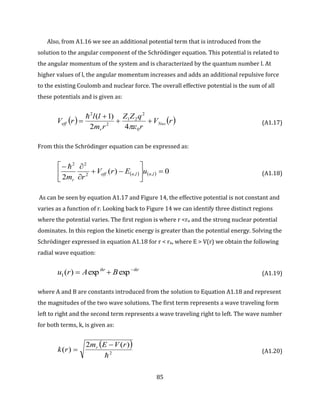
![81
With quantum mechanics, however, nuclei exhibit a wave/particle duality so that the
position of a particle has a probability of existing over a range of locations. Because of this
wave nature, the incident particle (X2) will have a finite probability of passing through the
Coulomb barrier even if its kinetic energy is much lower than the potential barrier. In
quantum mechanics, the behavior of a particle passing through a potential barrier where
the potential energy is greater than the kinetic energy is known as “tunneling.”
The tunneling probability for two nuclei was first derived by George Gamow in 1928
and his original approach is followed closely here[4]. The fusion problem can be
represented in quantum mechanics with the multi-particle Hamiltonian operator as a three
dimensional system comprised of particles X1 and X2 and the potential forces acting
between them. The system described by Figure 27 is represented in terms of the
Schrödinger equation as:
21212121
2
2
2
2
1
2
,,,,
22 21
rrrrrrrr
EV
mm
rr
(A1.4)
where m1 is the mass of X1, m2 is the mass of X2 , ψ(r1,r2) is the wave-function of the
system, V(r1,r2) is the total potential acting on the two particles (the sum of both the
nuclear and Coulomb potentials), and E is the kinetic energy of the system. The solution to
the Schrödinger equation that we seek is a wave-function, ψ(r1,r2), which contains all
information concerning the wave/particle nature of the interaction between the two
particles. The probability of X2 tunneling through the barrier and fusing with X1 can be
determined from the wave-function as will be shown later in the derivation.
The problem can be simplified significantly by representing equation A1.4 in the center
of mass frame of reference. In this reference it can be shown that the center of mass of the
system moves at a constant velocity. Because of this we can perform a Galilean coordinate
transformation from the original lab frame to a frame of reference on the center of mass
system where the origin of the new coordinate system is at the center of mass. In the center
of mass frame, the two particle system is represented as a single particle with mass mr that
is acted on by a central force whose origin is at the center of mass. Under the center of mass
representation, the Schrödinger equation in A1.4 becomes:](https://image.slidesharecdn.com/2ef4ba81-4ba4-4126-9f57-f636cceccd99-160618062518/85/WaughThesis-v2-2-81-320.jpg)
![84
2
2
2
2
2
sin
1
sin
sin
L (A1.13)
The eigenfuctions to the eigenvalue problem of equation A1.13 are given in the form of
spherical harmonics and can be represented using Legendre polynomials. The derivation of
the eigenfunctions is beyond the scope of the present derivation, but a complete derivation
can be found in standard introductory texts on quantum mechanics such as Liboff [55].The
eigenvalue solutions to the eigenvalue problem give the allowed values of the angular
momentum, L, of the system. The angular momentum can be expressed in terms of the
angular quantum number l and m, where the square of the angular momentum expressed
solely in terms of l is given as:
122
llL (A1.14)
Using A1.14 as the solution to the angular component, the complete Schrödinger equation
can be expressed in terms of the angular eigenvalue solution and radial eigenvalue problem
by combining A1.11, A1.13 and A1.14:
01
1
2
22
2
ErVrll
r
rR
r
rrRmr
(A1.15)
Finally, we can represent the radial component of the wave function by substituting
u(r)=R(r)·r into equation A1.15. Doing this we obtain:
0)(
2
)1(
2
,,2
2
2
22
lnln
rr
uErV
rm
ll
rm
(A1.16)
This result is much more straight forward and easier to work with. By recognizing the
angular invariance of the nuclear and Coulomb potentials, and representing the problem in
the center of mass frame, the whole system is reduced to a one dimensional problem with
an effective particle in the center of mass frame.](https://image.slidesharecdn.com/2ef4ba81-4ba4-4126-9f57-f636cceccd99-160618062518/85/WaughThesis-v2-2-84-320.jpg)

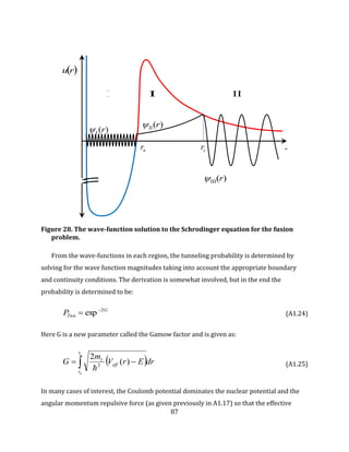
![90
Now consider the case where instead of two particles colliding, a single particle is launched
into a sea of target particles with density n2 [m-3]. The probability of a collision in this case
is given as the ratio of the surface area covered by target particles to the total area. This
ratio is given as:
dxn
A
dxAn
A
N
PRn
2
2
(A1.33)
where PRn is the probability of a reaction, N is the number of target particles, A is the area
of the incremental volume, n2 is the density of target particles, and dx is the differential
thickness of the volume. The situation is illustrated in Figure 30.
Figure 30. Fusion collisions with a density of target particles.
In this case the differential thickness of the reaction volume can be expressed in terms of
the velocity: dx = v·dt. By substituting into A1.33 and dividing by dt we get the single
particle reaction rate:
vn
dt
P
R Rn
2 (A1.34)
X
X
dx
A](https://image.slidesharecdn.com/2ef4ba81-4ba4-4126-9f57-f636cceccd99-160618062518/85/WaughThesis-v2-2-90-320.jpg)
![92
Appendix 2: MIT Linear Electrostatic Ion Accelerator (LEIA) Ion
Beam Current Measurements (Faraday Cup)
The MIT Linear Electrostatic Ion Accelerator (LEIA) [56] is a an accelerator-based fusion
product generator at the MIT Plasma Science and Fusion center that is primarily used for
nuclear diagnostic development for diagnostics fielded in the OMEGA [10] laser, the Z-
Machine [8], and the National Ignition Facility [9]. LEIA is capable of producing DD and
D3He fusion products at rates on the order of 107 s-1 and 106 s-1 respectively. An image of
LEIA is given in the figure below.
Figure 31. Linear Electrostatic Ion Accelerator (LEIA).
In the accelerator, DD or D3He gas is fed into a glass bottle that is ionized using an RF
source. After ionization, a ~5kV probe voltage is used to extract the ions from which they
are focused by a ~3.5kV focus supply and then accelerated down a 135kV acceleration
tube. The ions travel the length of the accelerator to the target chamber where the collide
with an erbium deuteride target creating DD or D3He fusion products depending on the gas
used and target doping (often times the target is doped with 3He and then hit with a D
beam to create D3He fusion products instead of running a 3He beam into the target
directly). Energies and yields from the charged particles are then measured using a surface
barrier semiconductor detector. A complete overview of LEIA can be found in Sinenian et.
al [56].](https://image.slidesharecdn.com/2ef4ba81-4ba4-4126-9f57-f636cceccd99-160618062518/85/WaughThesis-v2-2-92-320.jpg)

![106
SlitTCC
RCFSlitSlitTCC
Slit
RCF
L
LL
W
W
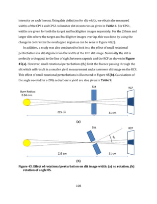
M
where RCFW is the width of the slit image on the RCF, SlitW is the actual width of the slit,
SlitTCCL is the distance from TCC to the slit, and RCFSlitL is the distance from the slit to the
RCF. The distance between TCC and the slit is documented for both CPS1 and CPS 2 where
SlitTCCL = 235cm for CPS1 and SlitTCCL = 100cm for CPS2. For CPS1, RCFSlitL has been
measured to be 31cm and the distance should be the same for CPS2 according to Damien
Hicks’ thesis[57], although this needs to be measured and verified. Magnification factors for
both CPS1 and CPS2 along with both experimental configurations are given in Figure 42.
Figure 42. Experimental configuration for CPS1 and CPS2 with corresponding
magnification factors.
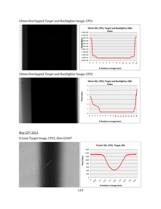
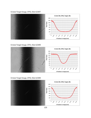
To obtain the slit width images for the 0.09mm to 2.0mm slits, the RCF was observed under
a microscope and a lineout was obtained by integrating the signal vertically over 1000
pixels to reduce noise. The slits 3.0mm and greater were too large to fit in a single frame
and instead were scanned to create an image containing multiple frames each at 100x
magnification. As each frame is 0.178mm wide at 100x magnification, the total width was
determined by multiplying the number of frames by the frame width. For slits 1.00mm and
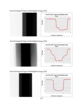
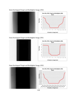
smaller, lineouts were made for both the target and backlighter slit images. For slits
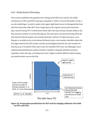
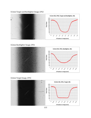
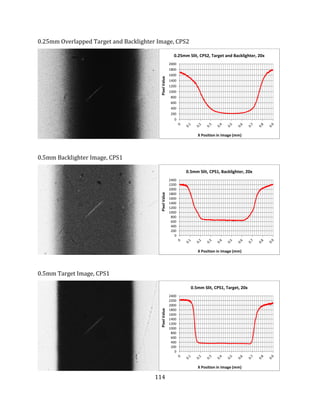
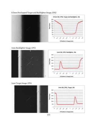
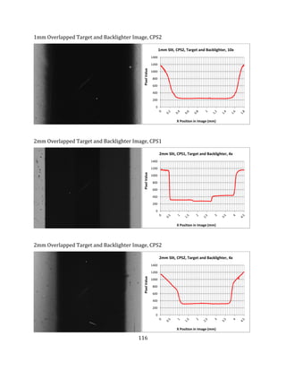
2.00mm and larger, a single lineout was made of the overlapping target and backlighter](https://image.slidesharecdn.com/2ef4ba81-4ba4-4126-9f57-f636cceccd99-160618062518/85/WaughThesis-v2-2-106-320.jpg)


![122
Appendix 4: Stage Etching of High Fluence Range Filter CR-39
Modules On Omega
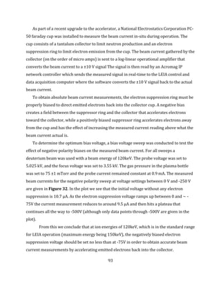
It has been shown previously that CR-39 solid state nuclear track plastic, used as a charged
particle detector on the “back-end” of OMEGA and NIF diagnostics/spectrometers, is ideally
suited to record particle fluences up to 3x10⁴ tracks/cm2 [31]. However, often times
conditions on OMEGA and the NIF can result in fluences two orders of magnitude greater
than this. Typically the optimal etch time for CR-39 to fully uncover charged particle tracks
is 5 hours. By using shorter etch times than the standard 5 hour, and by cross calibrating to
CR-39 shot on the MIT Linear Electrostatic Ion Accelerator (LEIA) to fluences equivalent to
what is seen on inertial confinement fusion experiments on OMEGA and the NIF, the
dynamic fluence range of the CR-39 can be significantly extended. Work conducted to
extend the range of the CR-39 fluence from OMEGA D3He exploding pusher shots is given
here for the case of DD and D3He protons.
Under standard conditions, CR-39 is etched in a solution of sodium hydroxide for 5
hours in order to full expose the charged particle tracks for detection under a 40x scanning
microscope and to etch the track diameters to a sufficient size so as to ensure good signal
to noise separation. An image depicting how the track diameter change as a function of etch
time is given in Figure 47. At a 5 hour etch, counting efficiencies of 100% are obtained
under both 40x and 100x magnification. Longer etch times are also beneficial for improving
signal to noise separation in the analysis. With fluences up to 3x10⁴/cm2, tracks are easily
distinguished and little overlap occurs. However, as the fluence increases beyond this,
tracks begin to overlap and are rejected by the scanning software as depicted in Figure 47.
The dynamic range of CR-39 can be significantly extended by reducing the etch time
which by so doing reduces the track diameter. However, if the etch time is reduce too much
the track will not be discerned by the scanning microscope which will result in track
undercounting and poor signal to noise separation. For a given fluence, then, there is an
optimal etch time span which is long enough so that track undercounting does not occur,
but at the same time is short enough so that tracks have not yet begun to overlap. An image](https://image.slidesharecdn.com/2ef4ba81-4ba4-4126-9f57-f636cceccd99-160618062518/85/WaughThesis-v2-2-122-320.jpg)
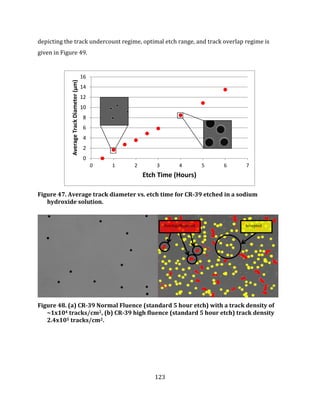
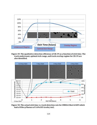

![126
Appendix 5: Absolute DDp Measurements taken on Exploding
Pushers on OMEGA (Febuary 7th and 9th, 2012)
This appendix documents the details of the analysis of CR-39 to obtain DD proton yields for use of
calibrating the OMEGA nTOF detector for Campaigns A and B for a series of shots conducted on
February 7th and 9th, 2012. For each analysis a header specified the following: TIM and trident
location of the CR-39 (e.g. TIM 1, 4:00), shot number, the amount of time (in hours) that the piece
was etched in a sodium hydroxide bath, the distance of the piece (in cm) from OMEGA TCC, and the
magnification used for the scanning software (standard being 40x). In addition, we include the
analysis parameters that specify the analysis software setup for analyzing both the 50μm and 25μm
steps. These parameters designate: Limit Area (the data area on the CR-39 to include in the
analysis), Background (the area on the CR-39 with no signal that is used for background
subtraction, Limit c% (the limit placed on the contrast of a track to aid in signal to noise
separation), Limit e% (the limit placed on the eccentricity of a track to aid in signal to noise
separation). Next, three plots are given to visualize the data by ploting all track by diameter vs.
eccentricit—N(d,c), diameter vs. contrast—N(d,e), and then just s histogram of track diameters. The
diameter vs. eccentricity and diameter vs. contrast are used to determine the signal to noise cutoffs
used in the analysis paramters (i.e. Limit c% and Limit e%). With signal separated from the noise,
an average track diameter is given along with a calculated track fluence in terms of tracks/cm2. The
yield is then obtained by multiplying the track fluence over the target chamber solid angle. For a
complete discussion on the analysis of charged particle tracks in CR-39 refer to Sequin et al. [31].](https://image.slidesharecdn.com/2ef4ba81-4ba4-4126-9f57-f636cceccd99-160618062518/85/WaughThesis-v2-2-126-320.jpg)

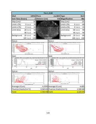
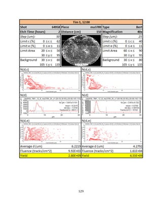
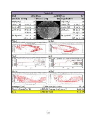
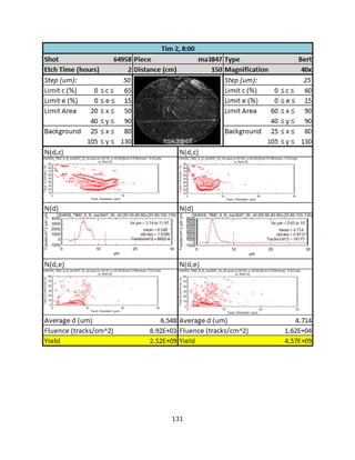
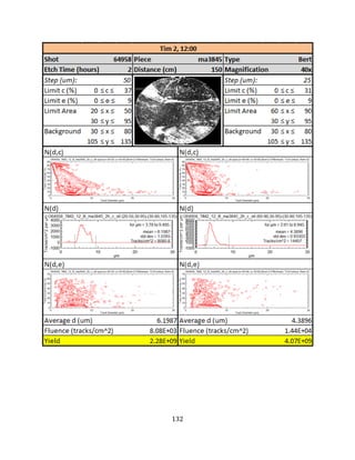
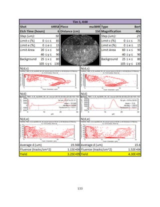
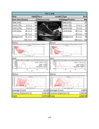
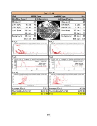
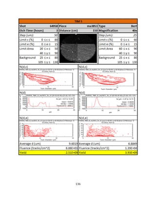
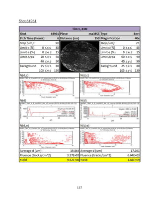

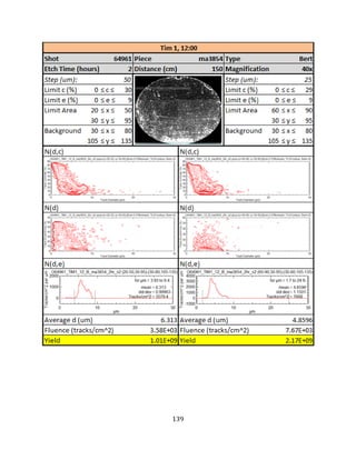
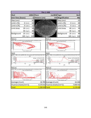

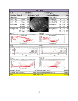
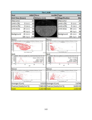
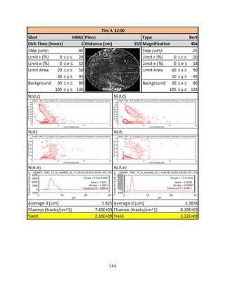
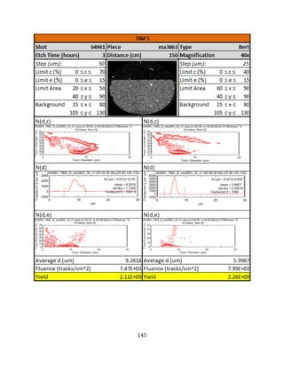
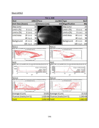
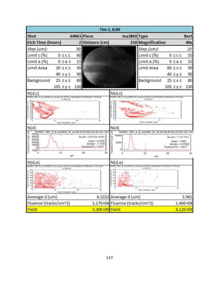
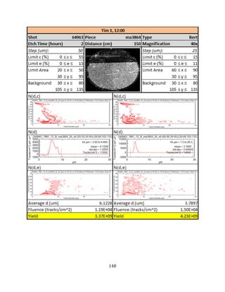
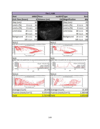
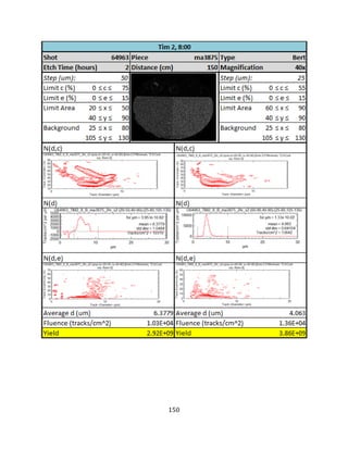
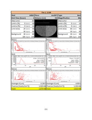
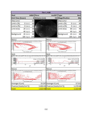
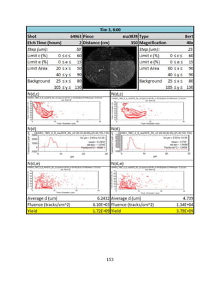
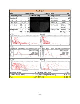
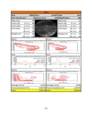
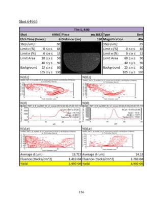
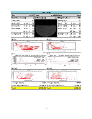
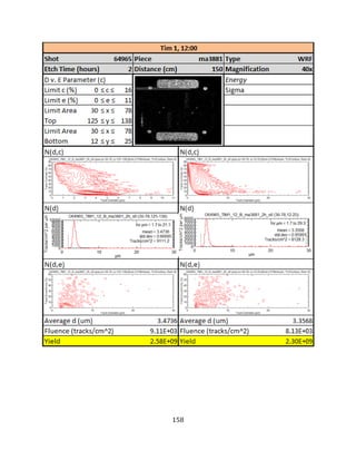
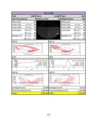
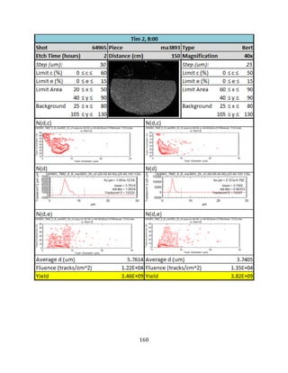
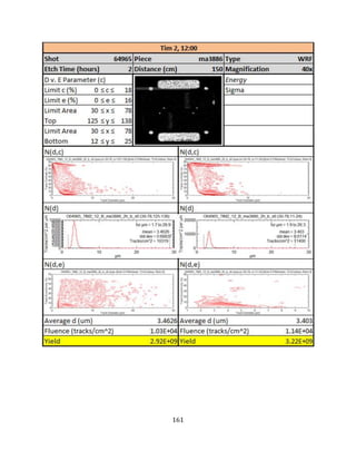
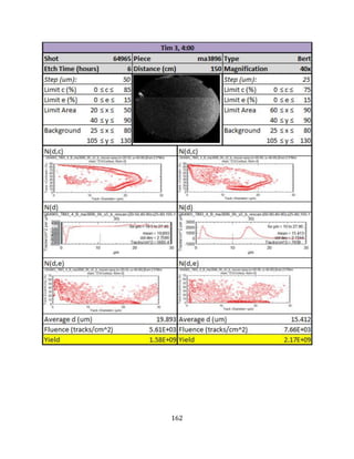
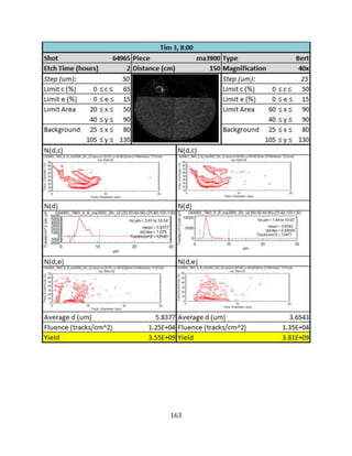
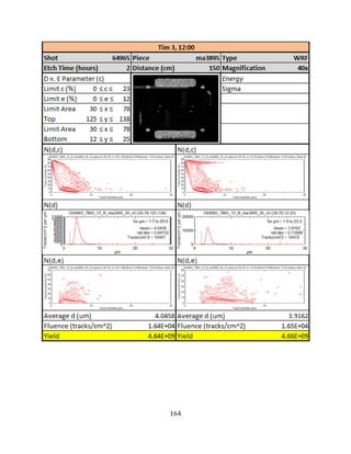
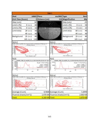


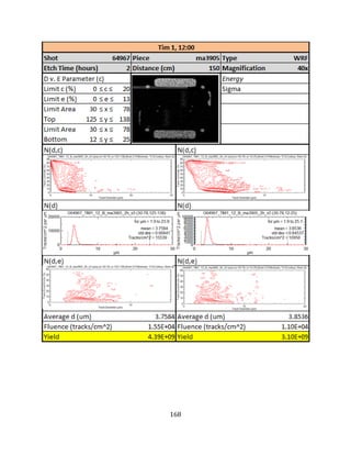
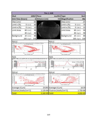
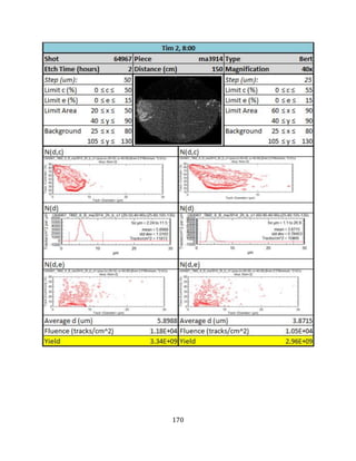
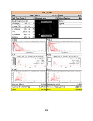
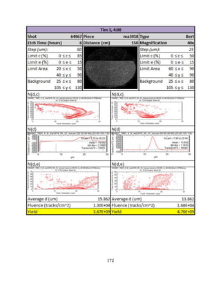
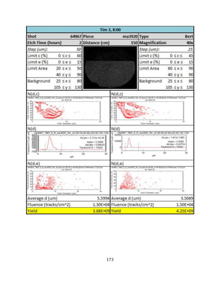
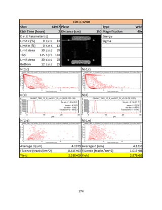
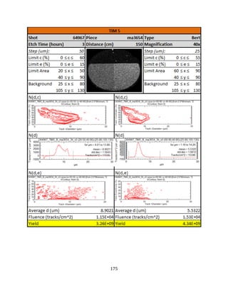
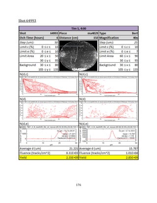
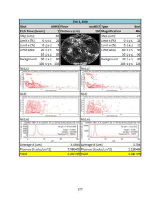
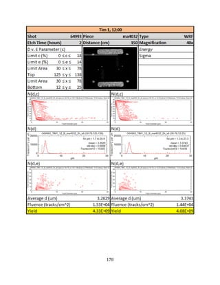
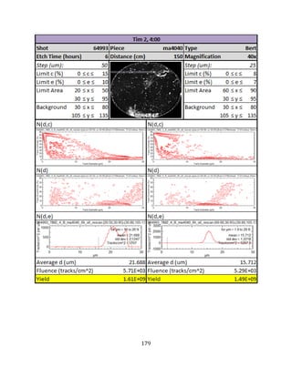
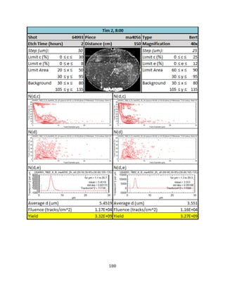
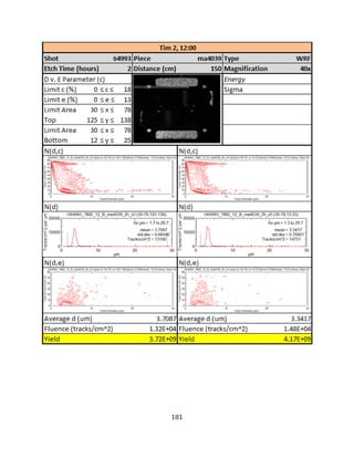
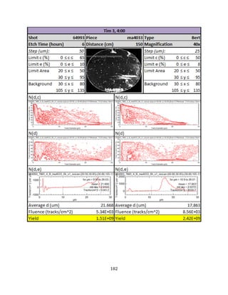
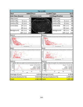

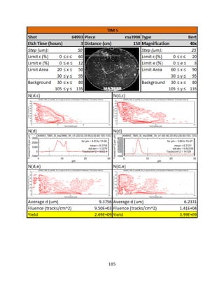
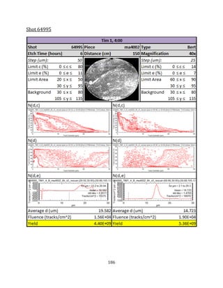
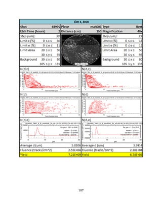
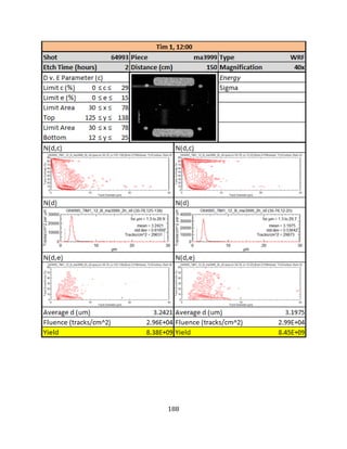
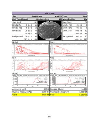
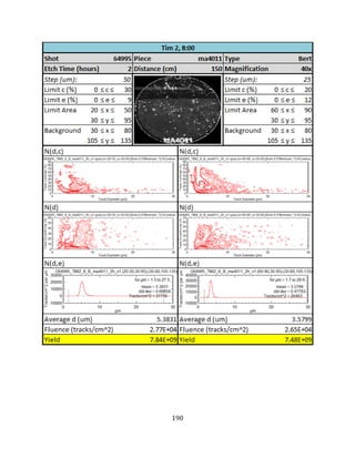
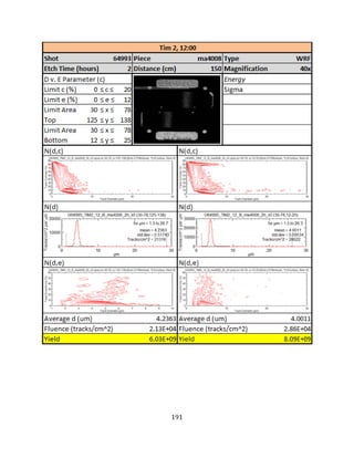
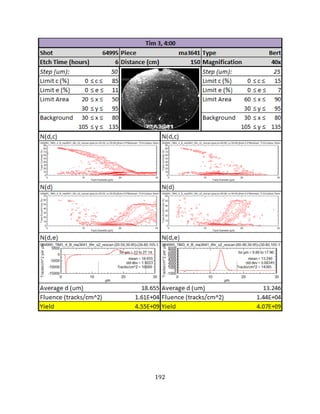
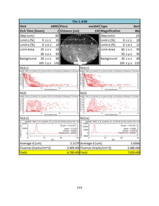
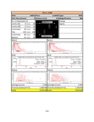
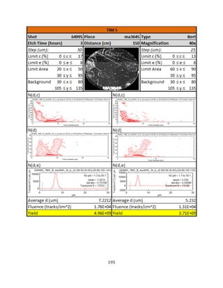
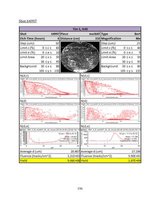
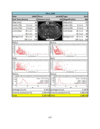
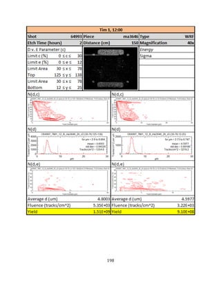
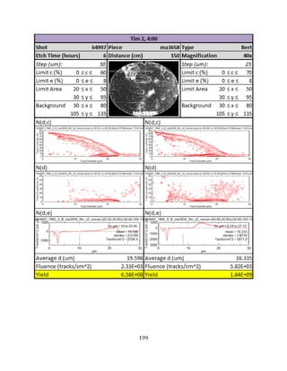
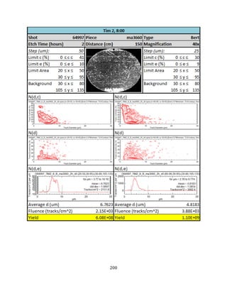
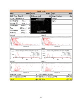
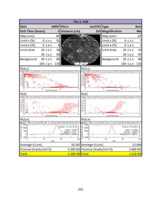
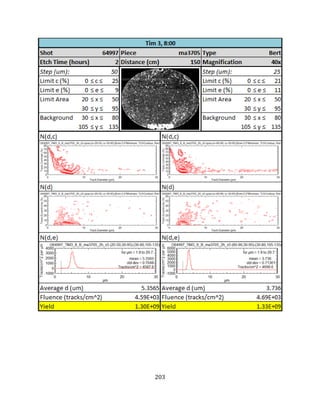
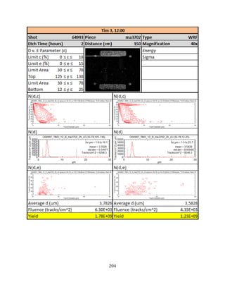
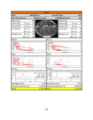
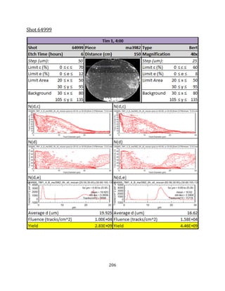
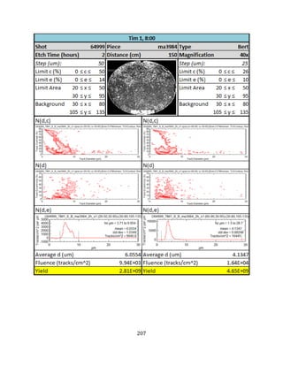
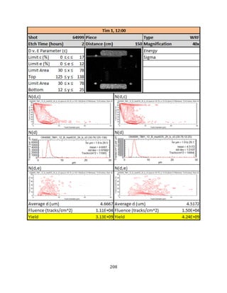
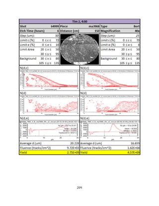
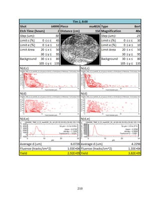

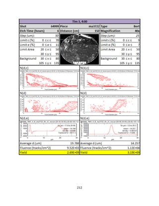


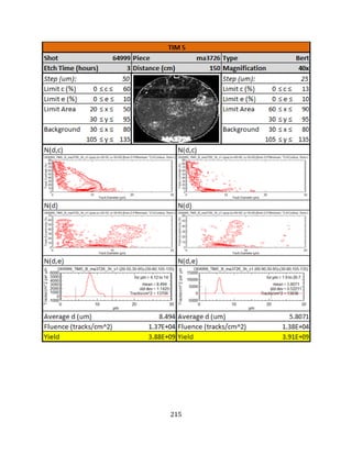
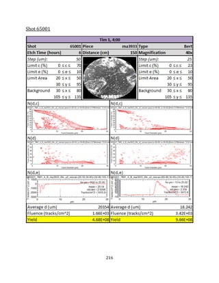
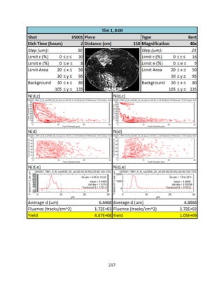
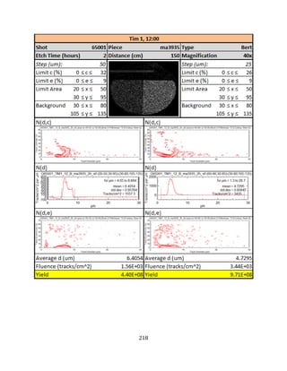
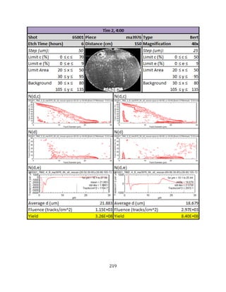
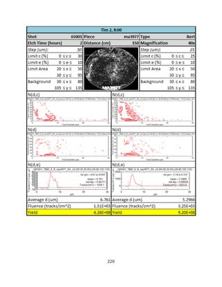
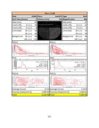
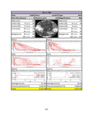
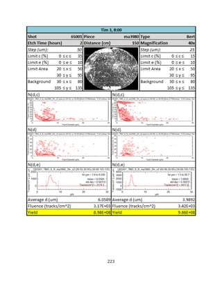
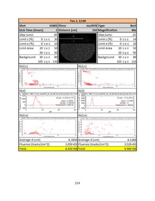
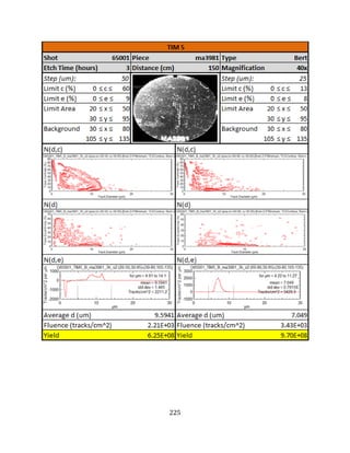


![[Phys 6006][Ben Williams][Inertial Confinement Fusion]](https://cdn.slidesharecdn.com/ss_thumbnails/ef672990-8608-4a95-b1ab-8afab317005e-150704125614-lva1-app6892-thumbnail.jpg?width=640&height=640&fit=bounds)


