Managerial economics

1. UNIT 2
Demand Analysis and
Forecasting
Dr. Nidhi Tewatia

2. Understanding the Demand
Function
• The demand function represents the mathematical relationship
between the quantity demanded of a product and its
determinants, such as price, income, prices of related goods, and
consumer preferences. It is typically expressed as:
• Q = f(P, Y, PR, T, O)
• Q: Quantity demanded of the product
• P: Price of the product
• Y: Consumer income
• PR: Prices of related goods (substitutes and complements)
• T: Tastes and preferences of consumers
• O: Other factors influencing demand (e.g., demographics,
advertising)

3. Factors Affecting Demand
1. Price: As the price of a product increases, the quantity demanded tends to decrease, assuming other factors
remain constant. This relationship is known as the law of demand.
2. Income: Changes in consumer income affect the demand for different goods. For normal goods, an increase
in income leads to an increase in the quantity demanded, while for inferior goods, the opposite is true.
3. Prices of Related Goods: The prices of substitutes and complements impact the demand for a product. If
the price of a substitute increases, the demand for the product may increase as consumers switch to the
cheaper alternative. Conversely, if the price of a complement increases, the demand for the product may
decrease.
A substitute good is a good that serves the same purpose as another good for consumers.
A complementary good is a good that adds value to another good when they are consumed together.
Pepsi and Coke are a typical example of substitute goods, whereas fries and ketchup may be considered
complements of each other.
4. Tastes and Preferences: Consumer preferences, influenced by factors like trends, advertising, and cultural
influences, play a significant role in shaping demand. Changes in tastes and preferences can lead to shifts in
the demand curve.
5. Other Factors: Various other factors, such as demographics, seasonality, technological advancements, and
government policies, can influence demand. For instance, changes in population demographics may affect the
demand for certain products or services.

4. Law of Demand
• The law of demand states that the quantity demanded of a
good shows an inverse relationship with the price of a good
when other factors are held constant (cetris peribus). It
means that as the price increases, demand decreases.
• The law of demand is a fundamental principle in
macroeconomics. It is used together with the law of supply
to determine the efficient allocation of resources in an
economy and find the optimal price and quantity of goods.

5. Graphical Representation of the Law of Demand
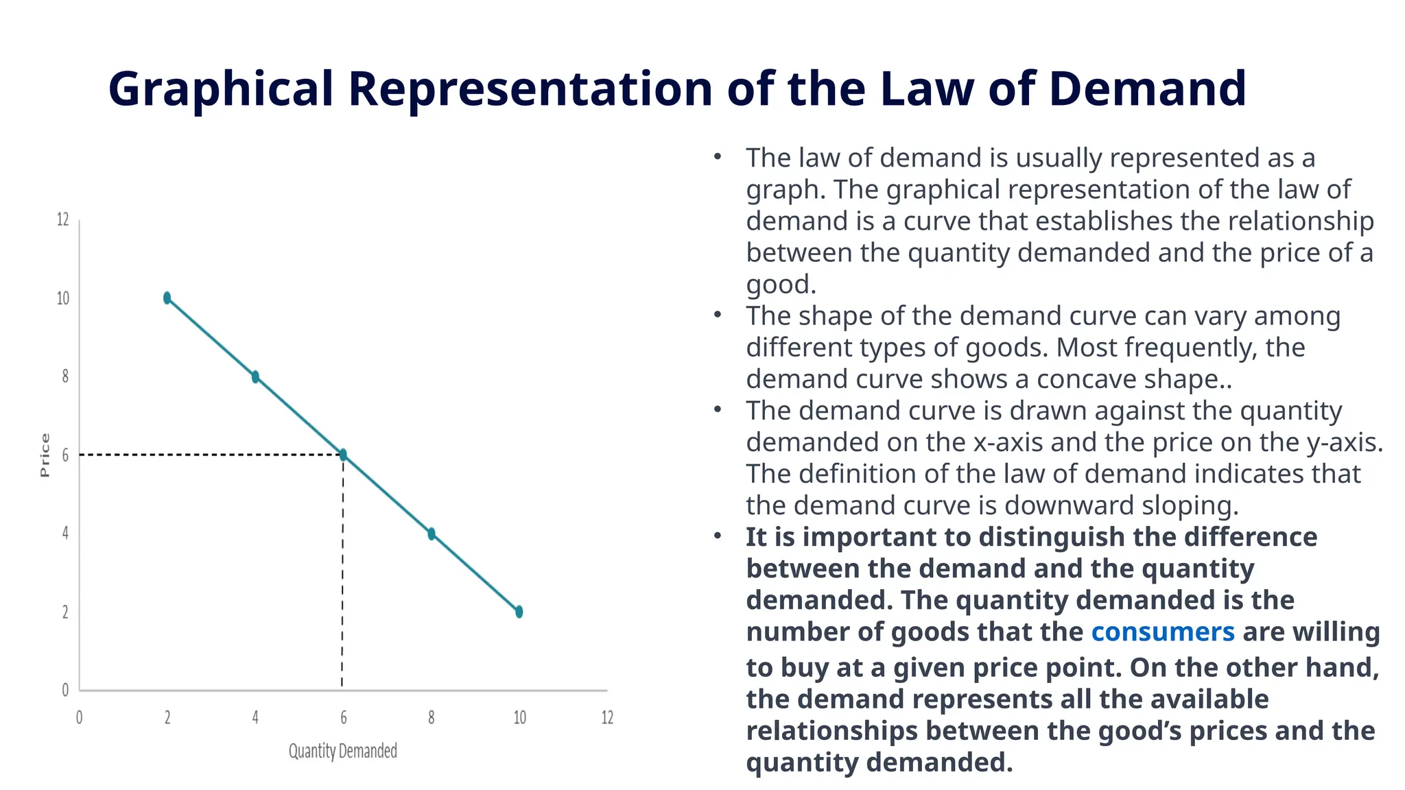
• The law of demand is usually represented as a
graph. The graphical representation of the law of
demand is a curve that establishes the relationship
between the quantity demanded and the price of a
good.
• The shape of the demand curve can vary among
different types of goods. Most frequently, the
demand curve shows a concave shape..
• The demand curve is drawn against the quantity
demanded on the x-axis and the price on the y-axis.
The definition of the law of demand indicates that
the demand curve is downward sloping.
• It is important to distinguish the difference
between the demand and the quantity
demanded. The quantity demanded is the
number of goods that the consumers are willing
to buy at a given price point. On the other hand,
the demand represents all the available
relationships between the good’s prices and the
quantity demanded.

6. Types of Demand
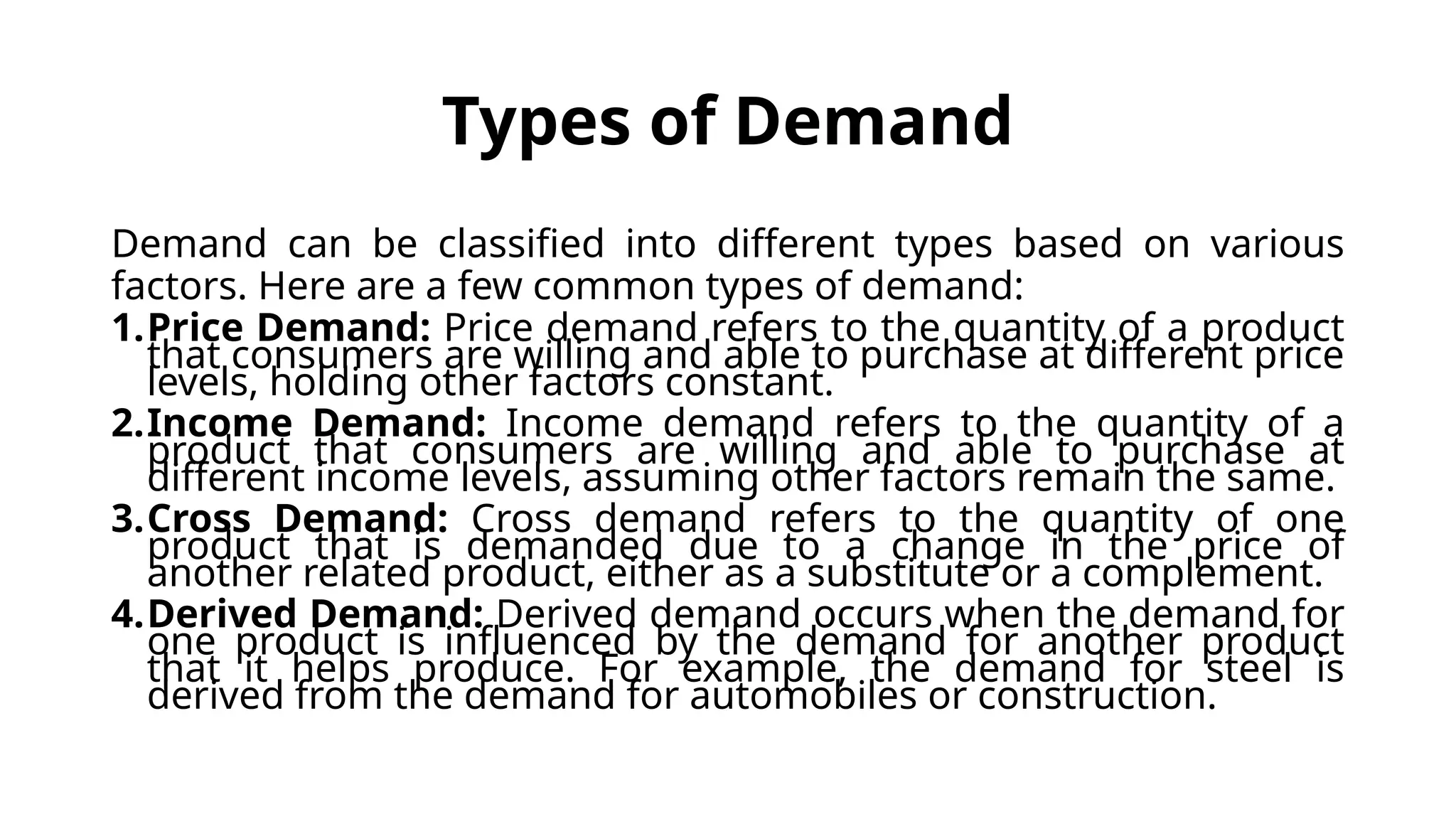
Demand can be classified into different types based on various
factors. Here are a few common types of demand:
1.Price Demand: Price demand refers to the quantity of a product
that consumers are willing and able to purchase at different price
levels, holding other factors constant.
2.Income Demand: Income demand refers to the quantity of a
product that consumers are willing and able to purchase at
different income levels, assuming other factors remain the same.
3.Cross Demand: Cross demand refers to the quantity of one
product that is demanded due to a change in the price of
another related product, either as a substitute or a complement.
4.Derived Demand: Derived demand occurs when the demand for
one product is influenced by the demand for another product
that it helps produce. For example, the demand for steel is
derived from the demand for automobiles or construction.

7. 5.Elastic Demand: Elastic demand refers to a situation where
a change in price leads to a relatively larger change in
quantity demanded. In elastic demand, consumers are highly
responsive to price changes.
6.Inelastic Demand: In contrast to elastic demand, inelastic
demand refers to a situation where a change in price leads to
a relatively smaller change in quantity demanded. In this
case, consumers are less responsive to price changes.

8. Exceptions to the Law of Demand
• Unlike the laws of mathematics or physics, the laws of economics are not universal. For example,
the law of demand comes with a few exceptions. Some goods do not show an inverse relationship
between the price and the quantity. Therefore, the demand curve for these goods is upward-
sloping.
1. Giffen goods
• These are inferior goods that lack close substitutes that represent a large portion of the consumer’s
income. Scottish economist Sir Robert Giffen proposed the existence of such goods in the
19th
century. Giffen goods violate the law of demand because the prices of these goods increase
with the increase in the quantity demanded. However, Giffen goods remain mostly a theoretical
concept as there is limited empirical evidence of their existence in the real world.
2. Veblen goods
• Certain types of luxury goods violate the law of demand. Veblen goods are named after American
economist Thorstein Veblen. Generally, they are luxury goods that indicate the economic and social
status of the owner. Therefore, consumers are willing to consume Veblen goods even more when
the price increases. Some examples of Veblen goods include luxury cars, expensive wines, and
designer clothes.

9. Movement of the Demand Curve
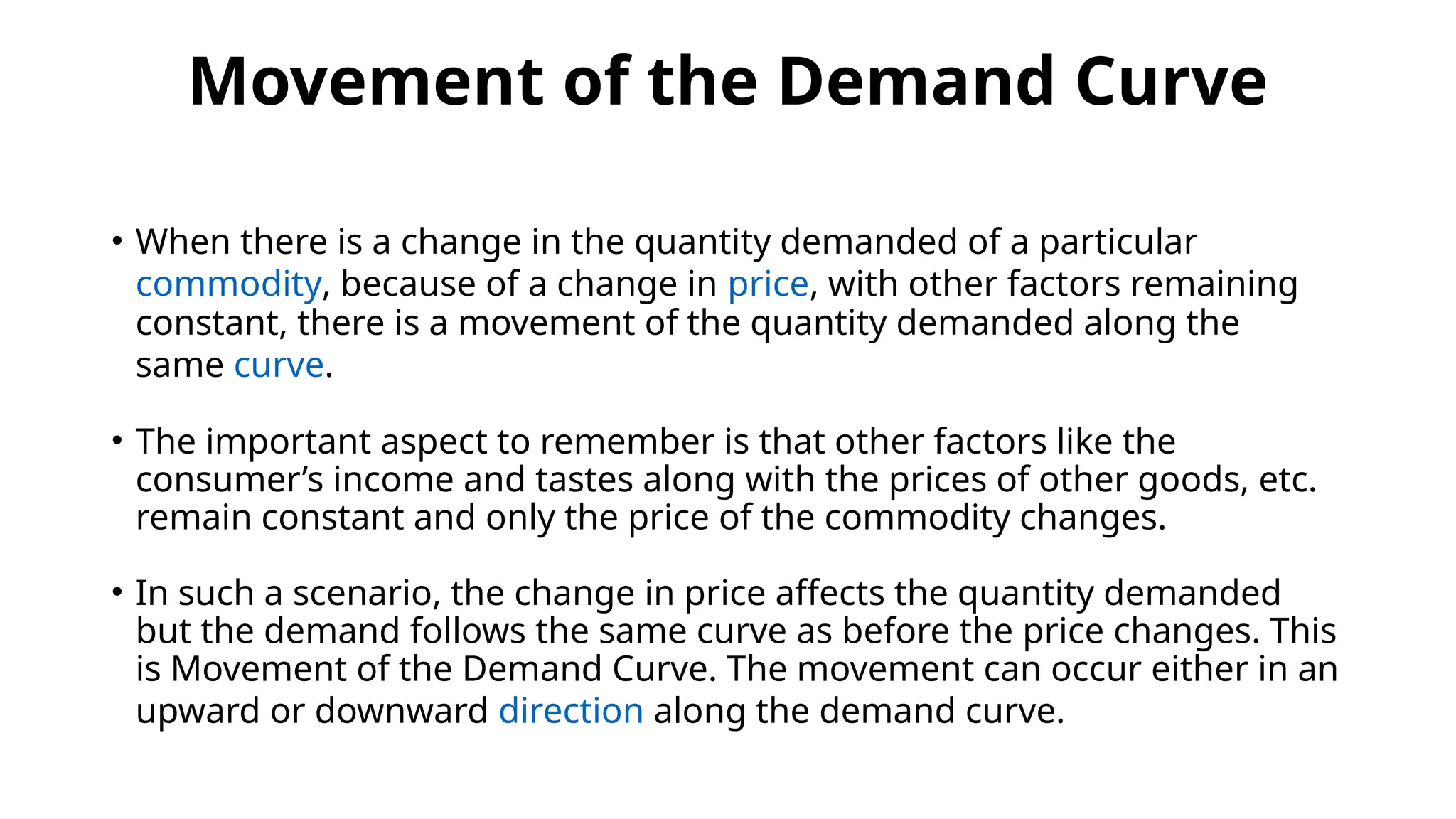
• When there is a change in the quantity demanded of a particular
commodity, because of a change in price, with other factors remaining
constant, there is a movement of the quantity demanded along the
same curve.
• The important aspect to remember is that other factors like the
consumer’s income and tastes along with the prices of other goods, etc.
remain constant and only the price of the commodity changes.
• In such a scenario, the change in price affects the quantity demanded
but the demand follows the same curve as before the price changes. This
is Movement of the Demand Curve. The movement can occur either in an
upward or downward direction along the demand curve.

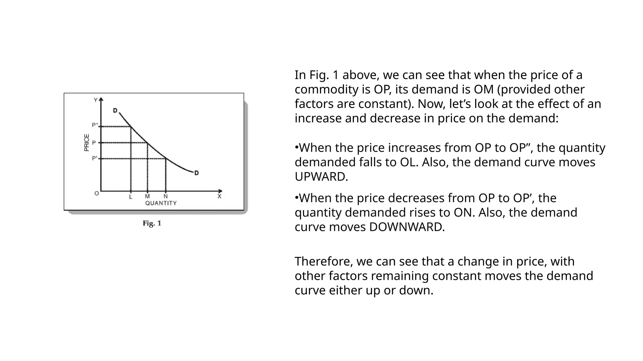
10. In Fig. 1 above, we can see that when the price of a
commodity is OP, its demand is OM (provided other
factors are constant). Now, let’s look at the effect of an
increase and decrease in price on the demand:
•When the price increases from OP to OP”, the quantity
demanded falls to OL. Also, the demand curve moves
UPWARD.
•When the price decreases from OP to OP’, the
quantity demanded rises to ON. Also, the demand
curve moves DOWNWARD.
Therefore, we can see that a change in price, with
other factors remaining constant moves the demand
curve either up or down.

11. The shift of the Demand Curve
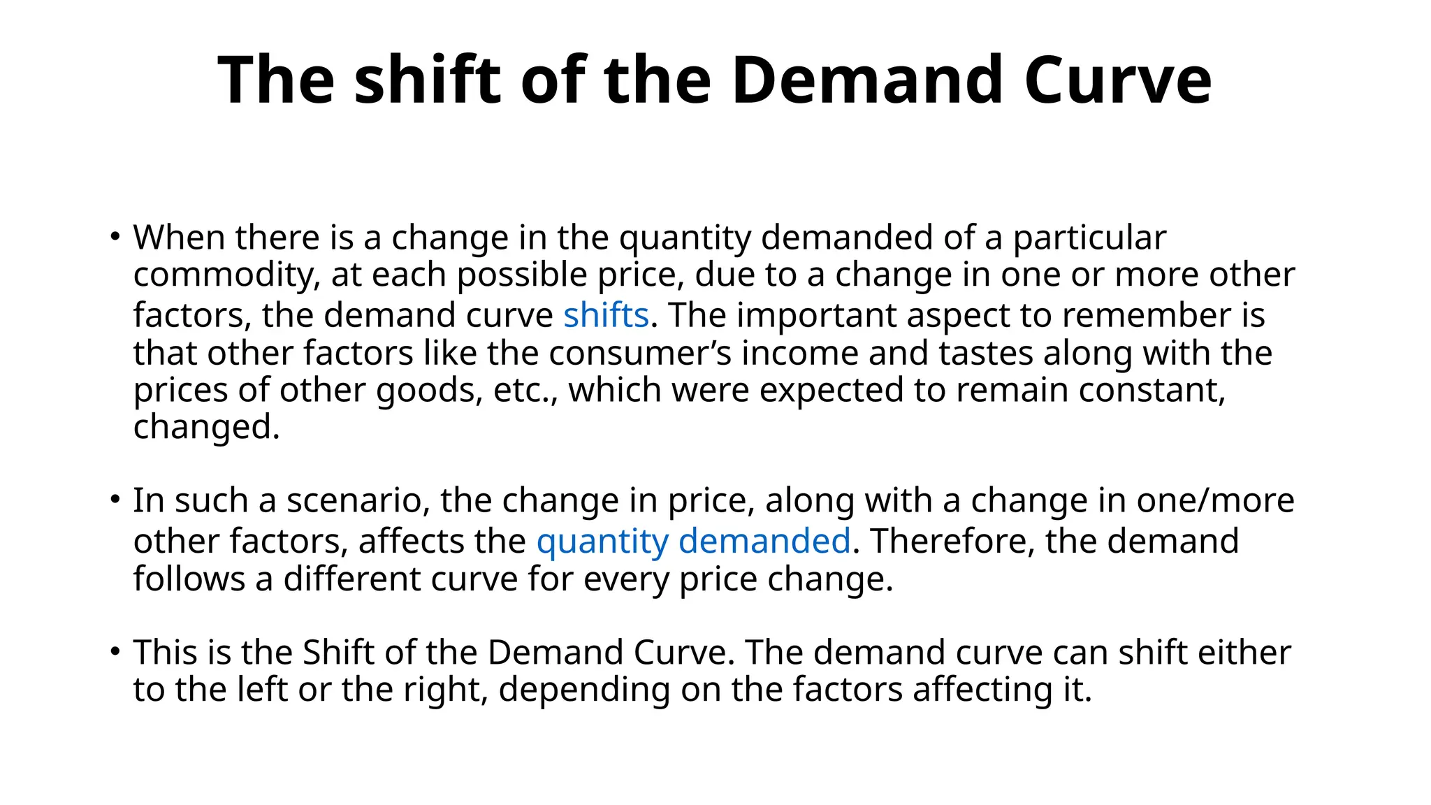
• When there is a change in the quantity demanded of a particular
commodity, at each possible price, due to a change in one or more other
factors, the demand curve shifts. The important aspect to remember is
that other factors like the consumer’s income and tastes along with the
prices of other goods, etc., which were expected to remain constant,
changed.
• In such a scenario, the change in price, along with a change in one/more
other factors, affects the quantity demanded. Therefore, the demand
follows a different curve for every price change.
• This is the Shift of the Demand Curve. The demand curve can shift either
to the left or the right, depending on the factors affecting it.

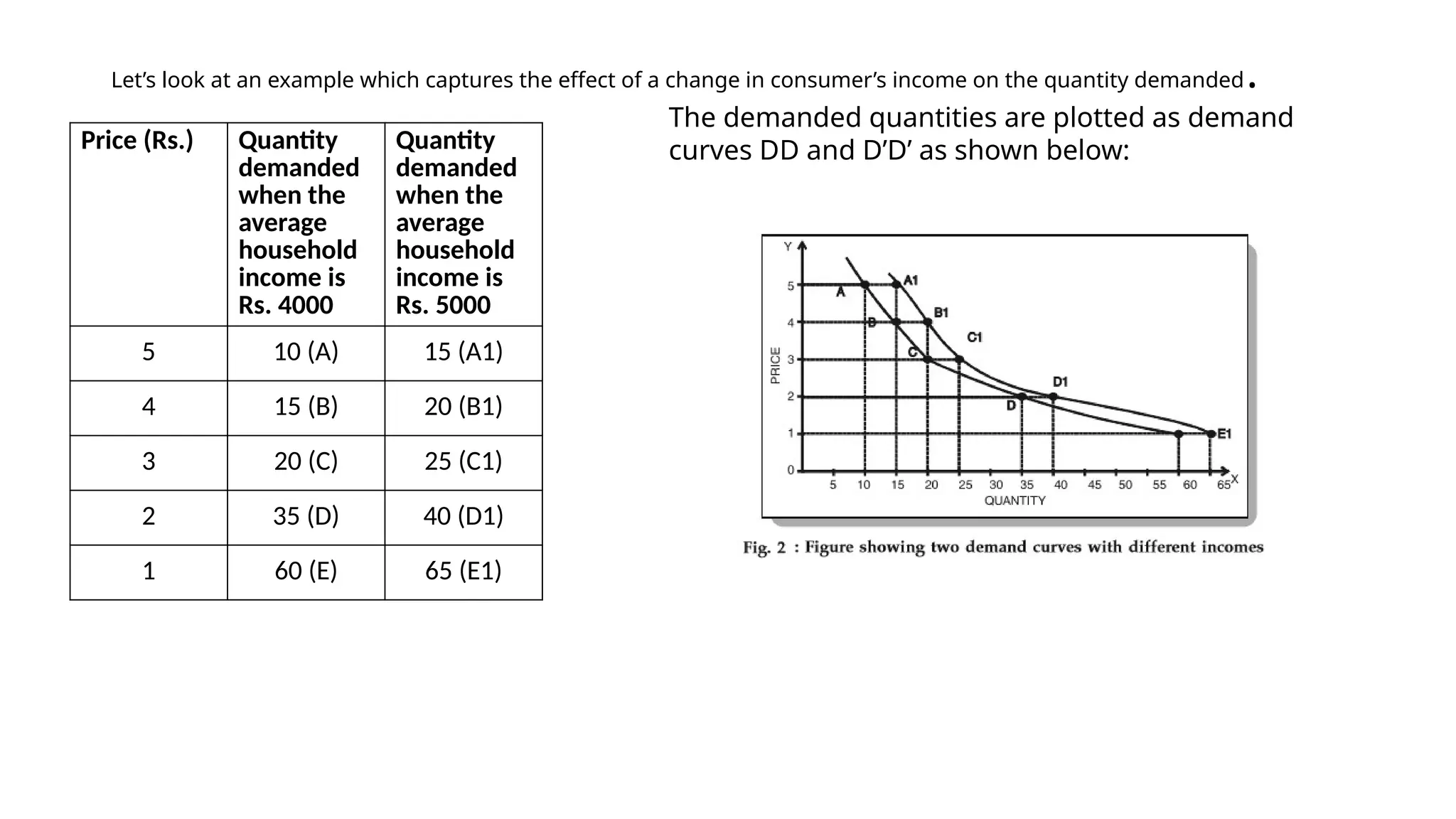
12. Let’s look at an example which captures the effect of a change in consumer’s income on the quantity demanded.
Price (Rs.) Quantity
demanded
when the
average
household
income is
Rs. 4000
Quantity
demanded
when the
average
household
income is
Rs. 5000
5 10 (A) 15 (A1)
4 15 (B) 20 (B1)
3 20 (C) 25 (C1)
2 35 (D) 40 (D1)
1 60 (E) 65 (E1)
The demanded quantities are plotted as demand
curves DD and D’D’ as shown below:

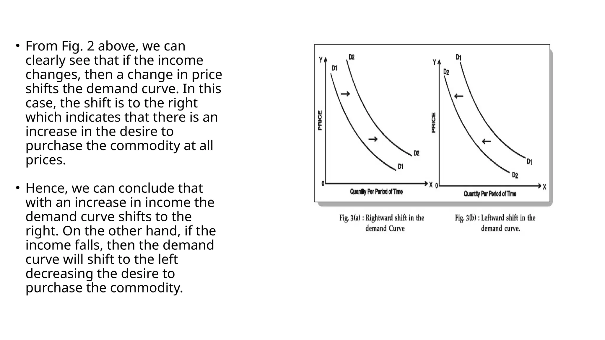
13. • From Fig. 2 above, we can
clearly see that if the income
changes, then a change in price
shifts the demand curve. In this
case, the shift is to the right
which indicates that there is an
increase in the desire to
purchase the commodity at all
prices.
• Hence, we can conclude that
with an increase in income the
demand curve shifts to the
right. On the other hand, if the
income falls, then the demand
curve will shift to the left
decreasing the desire to
purchase the commodity.

14. Bandwagon Effect & Snob Effect;
• Bandwagon Effect: - The bandwagon effect is a well-documented form of group think in behavioral science
and has many applications. Some of the people purchase commodity not because of necessity but because
their neighbours have bought these goods. It is otherwise called as Band-Wagon effect. These effects have
positive effect on demand. The tendency to follow the actions or beliefs of others can occur because
individuals directly prefer to conform, or because individuals derive information from others. In layman’s
term the bandwagon effect refers to people doing certain things because other people are doing them,
regardless of their ow n beliefs, which they may ignore or override.
For example, people might buy a new electronic item because of its popularity, regardless of whether they need
it, can afford it, or even really want it.
• Snob Effect: - when the commodities are commonly used rich class people decrease the consumption. Or
there are also consumers who like to behave differently from the others. This is known as Snob effect and it
has negative effect on demand. This situation is derived by the desire too have unusual, expensive or unique
goods.
Example - Designer clothing: People may buy designer clothing to signal their wealth and sophistication.
Rare art: People may buy rare works of art to signal their wealth and sophistication.

15. Elasticity of Demand
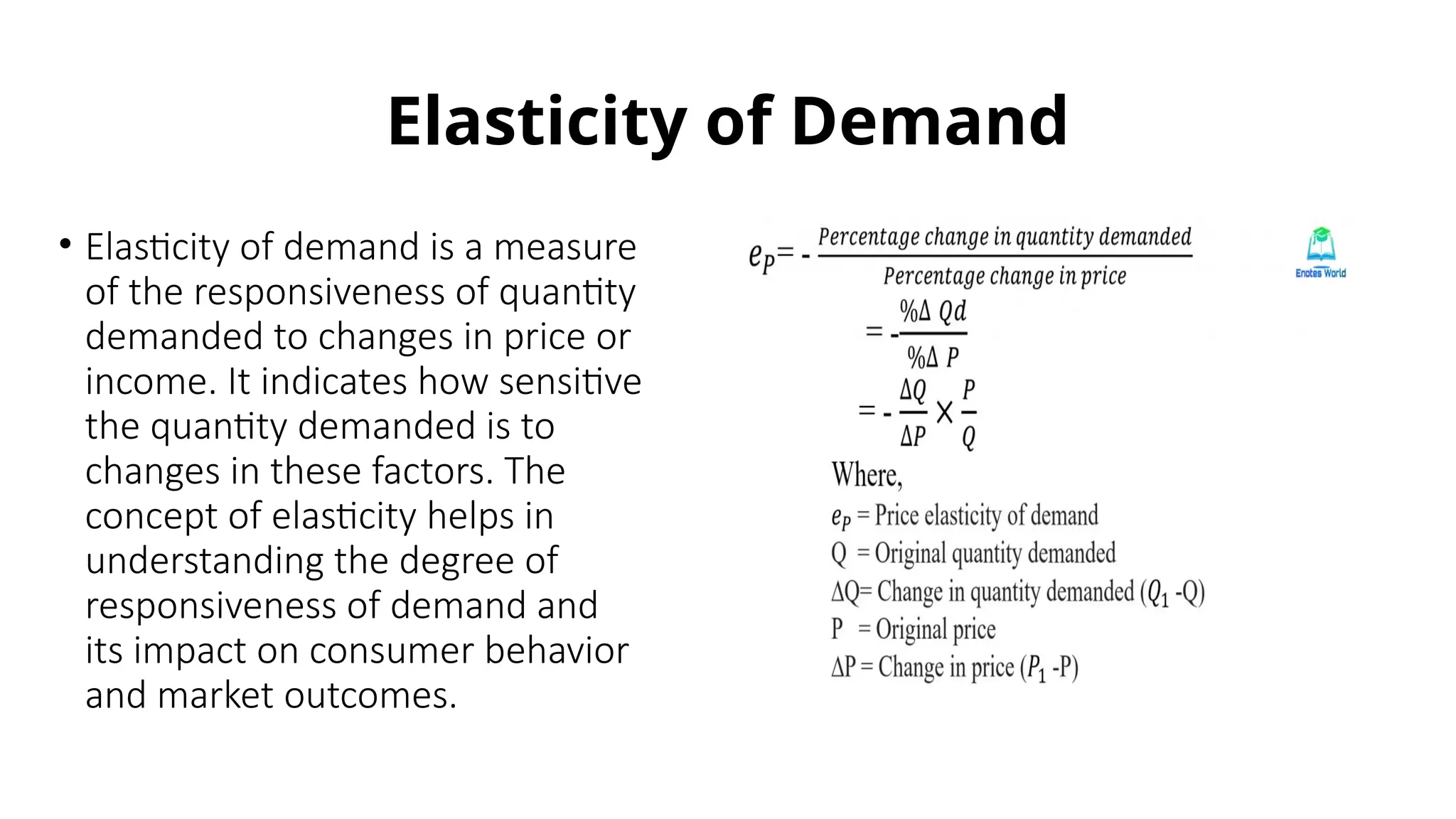
• Elasticity of demand is a measure
of the responsiveness of quantity
demanded to changes in price or
income. It indicates how sensitive
the quantity demanded is to
changes in these factors. The
concept of elasticity helps in
understanding the degree of
responsiveness of demand and
its impact on consumer behavior
and market outcomes.

16. Elastic Demand
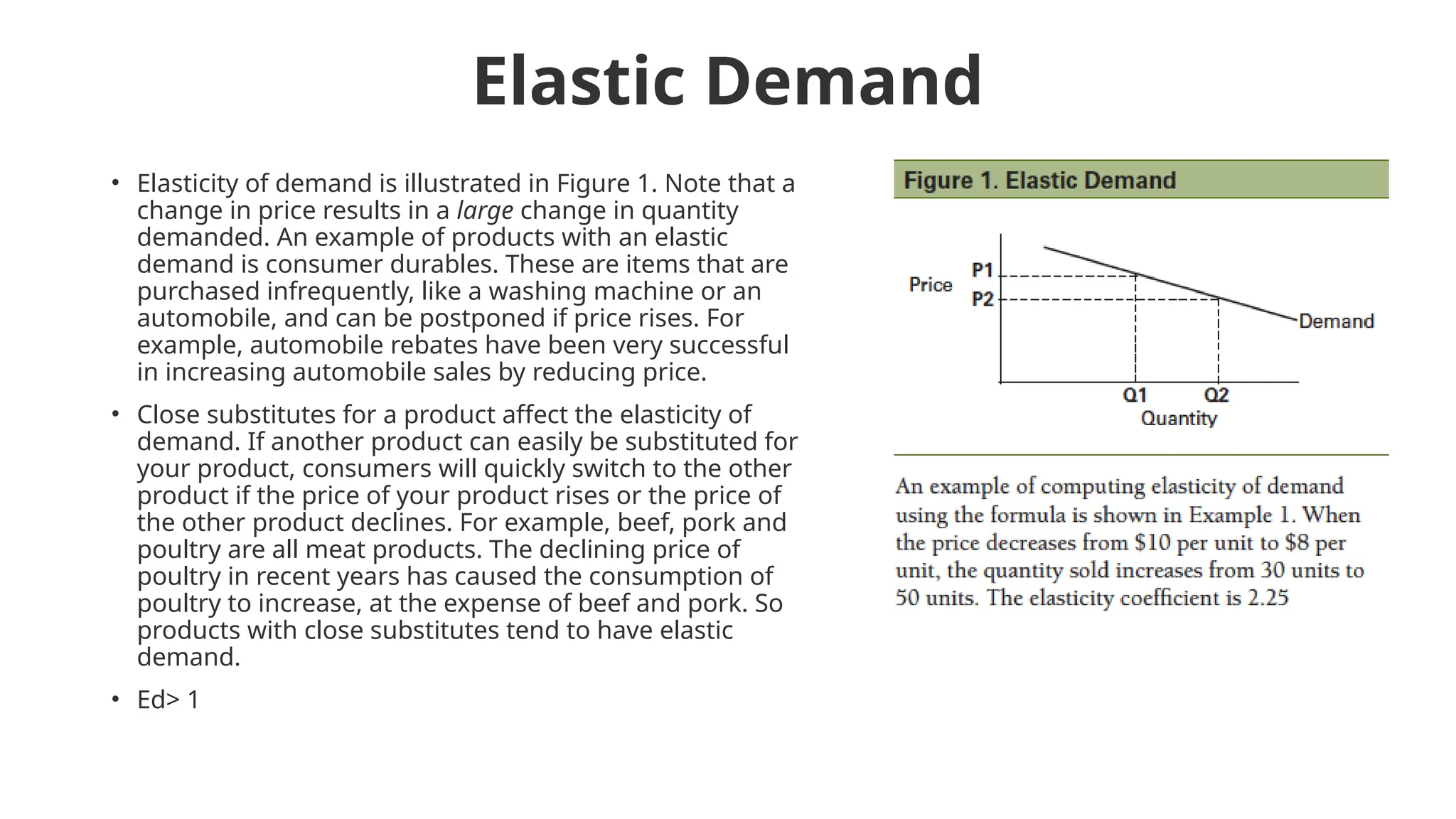
• Elasticity of demand is illustrated in Figure 1. Note that a
change in price results in a large change in quantity
demanded. An example of products with an elastic
demand is consumer durables. These are items that are
purchased infrequently, like a washing machine or an
automobile, and can be postponed if price rises. For
example, automobile rebates have been very successful
in increasing automobile sales by reducing price.
• Close substitutes for a product affect the elasticity of
demand. If another product can easily be substituted for
your product, consumers will quickly switch to the other
product if the price of your product rises or the price of
the other product declines. For example, beef, pork and
poultry are all meat products. The declining price of
poultry in recent years has caused the consumption of
poultry to increase, at the expense of beef and pork. So
products with close substitutes tend to have elastic
demand.
• Ed> 1

17. Inelastic Demand
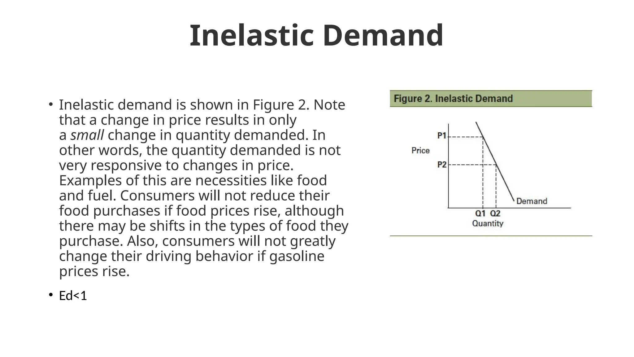
• Inelastic demand is shown in Figure 2. Note
that a change in price results in only
a small change in quantity demanded. In
other words, the quantity demanded is not
very responsive to changes in price.
Examples of this are necessities like food
and fuel. Consumers will not reduce their
food purchases if food prices rise, although
there may be shifts in the types of food they
purchase. Also, consumers will not greatly
change their driving behavior if gasoline
prices rise.
• Ed<1

18. Unitary Elasticity
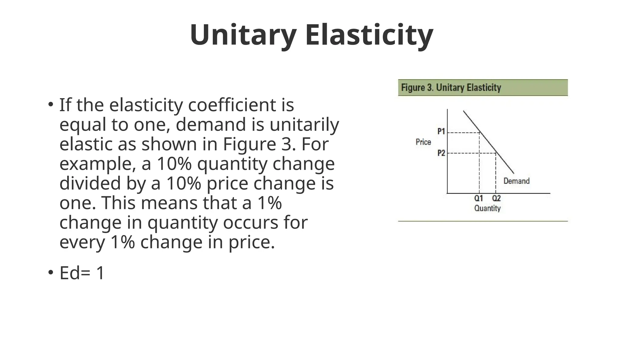
• If the elasticity coefficient is
equal to one, demand is unitarily
elastic as shown in Figure 3. For
example, a 10% quantity change
divided by a 10% price change is
one. This means that a 1%
change in quantity occurs for
every 1% change in price.
• Ed= 1

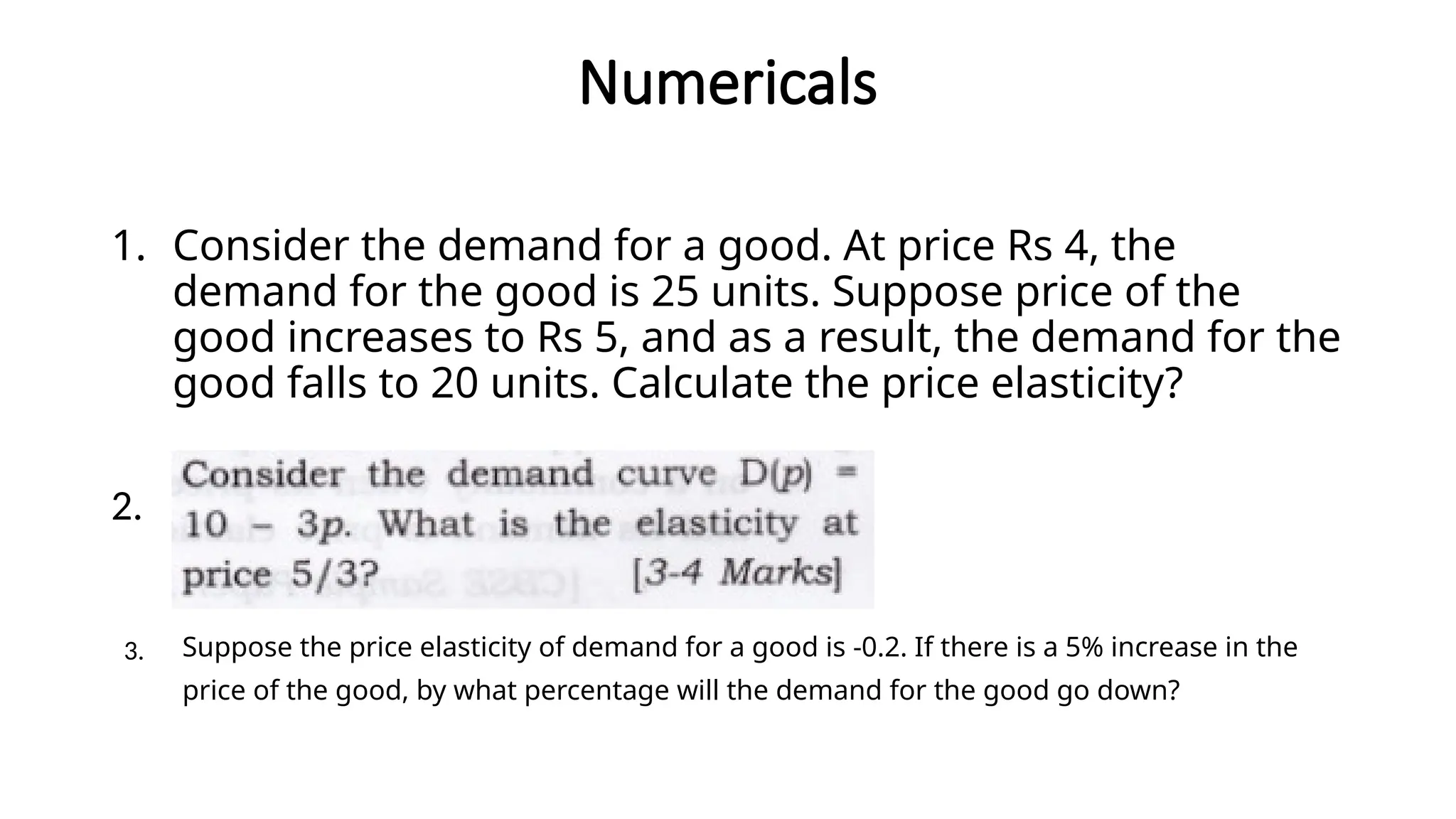
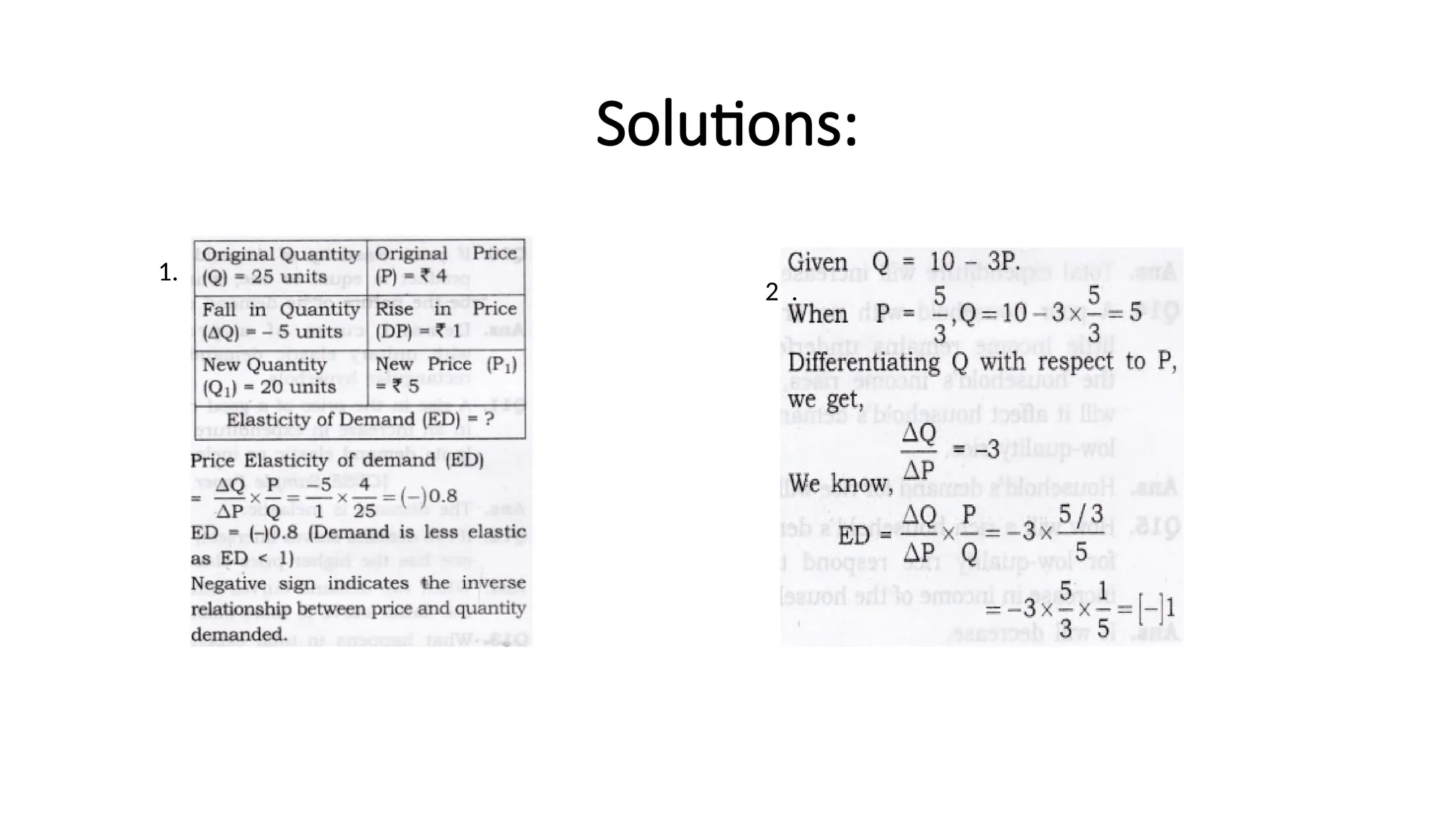
19. Numericals
1. Consider the demand for a good. At price Rs 4, the
demand for the good is 25 units. Suppose price of the
good increases to Rs 5, and as a result, the demand for the
good falls to 20 units. Calculate the price elasticity?
2.
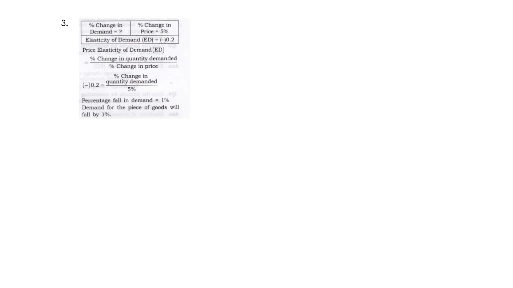
Suppose the price elasticity of demand for a good is -0.2. If there is a 5% increase in the
price of the good, by what percentage will the demand for the good go down?
3.

20. Solutions:
1.
2 .

21. 3.

22. ESTIMATING DEMAND USING REGRESSION ANALYSIS
• Estimating demand is a critical aspect of managerial
economics that helps businesses make informed decisions
about pricing, production, and marketing strategies.
Regression analysis is a widely used statistical technique
that allows businesses to estimate demand by analyzing the
relationship between the quantity demanded of a product
and its key determinants.

23. Estimating Demand Using Regression Analysis
EstimUnderstanding Regression Analysis
ting Demand Using Regression Analysis
• Regression analysis is a statistical technique that examines the
relationship between a dependent variable and one or more
independent variables. In the context of demand estimation, the
dependent variable is the quantity demanded of a product, while
the independent variables are factors that influence demand, such
as price, income, advertising expenditure, and competitor’s price.
• By analyzing historical data on the quantity demanded and the
corresponding values of the independent variables, regression
analysis allows businesses to quantify the impact of these
variables on demand and develop an equation that can be used to
estimate future demand.

24. Advantages of Demand Estimation Using Regression
Analysis
1.Quantitative Analysis: Regression analysis provides a quantitative approach to estimating
demand, allowing businesses to obtain numerical estimates of the impact of different
factors on demand. This helps in making more precise and data-driven decisions.
2.Identification of Key Determinants: Regression analysis helps identify the key
determinants of demand by examining the relationship between the dependent variable
(quantity demanded) and the independent variables (factors affecting demand). This
understanding allows businesses to focus their efforts on the most influential factors when
developing strategies.
3.Forecasting: Once the demand equation is established using regression analysis,
businesses can utilize it for demand forecasting. By inputting values of the independent
variables into the equation, they can estimate the quantity demanded under different
scenarios, aiding in production planning, resource allocation, and inventory management.
4.Sensitivity Analysis: Regression analysis enables businesses to conduct sensitivity analysis
by assessing the responsiveness of demand to changes in independent variables. This
information helps in understanding the elasticity of demand and the potential impact of
pricing, advertising, or other strategic decisions on quantity demanded.

25. Steps in Conducting Demand
Estimation Using Regression
Analysis
1.Data Collection: Gather historical data on the quantity demanded
and relevant independent variables, such as price, income,
advertising expenditure, and competitor’s price. Ensure that an
adequate amount of data is collected to capture variations in the
variables over time.
2.Specification of the Regression Equation: Based on economic
theory and knowledge of the industry, determine the form of the
regression equation. For example, if price is expected to have a linear
relationship with quantity demanded, the equation might take the
form: Quantity Demanded = β0 + β1 * Price + ε, where β0 and β1 are
the coefficients to be estimated, and ε is the error term.

26. 3. Estimation of Coefficients: Use statistical software or
tools to estimate the coefficients of the regression equation.
The estimation process involves minimizing the sum of
squared differences between the observed quantity
demanded and the values predicted by the equation.
4. Interpretation of Coefficients: Interpret the estimated
coefficients to understand the impact of each independent
variable on demand. Positive coefficients indicate a positive
relationship with demand, while negative coefficients indicate
an inverse relationship.
5.Utilization and Analysis: Once the demand equation is
validated, utilize it to estimate demand under different
scenarios, conduct sensitivity analysis, and support decision-
making processes related to pricing, production, and
marketing strategies.

27. Demand forecasting
• Demand forecasting is a critical aspect of managerial
economics that helps businesses estimate future consumer
demand for their products or services. Accurate demand
forecasting enables businesses to make informed decisions
about production planning, inventory management, pricing
strategies, and resource allocation. In this , we will explore
some commonly used demand forecasting techniques and
their application in business.

28. Time Series Analysis
• Time series analysis is a widely used technique for demand forecasting, especially when
historical data is available. It involves analyzing past demand patterns to identify
trends, seasonality, and other recurring patterns that can be used to make future
predictions. Time series analysis techniques include:
1.Moving Averages: Moving averages calculate the average demand over a specified
period, smoothing out short-term fluctuations. Simple moving averages use a fixed
time period, while weighted moving averages assign different weights to each data
point based on their significance.
2.Exponential Smoothing: Exponential smoothing assigns exponentially declining
weights to past demand observations, giving more weight to recent data. This
technique is useful for capturing short-term changes in demand.
3.ARIMA Models: ARIMA (Auto Regressive Integrated Moving Average) models combine
autoregressive (This component represents the relationship between the current value and past
values) and moving average components to model and forecast time series data. They
can capture trends, seasonality, and irregularities in demand patterns.

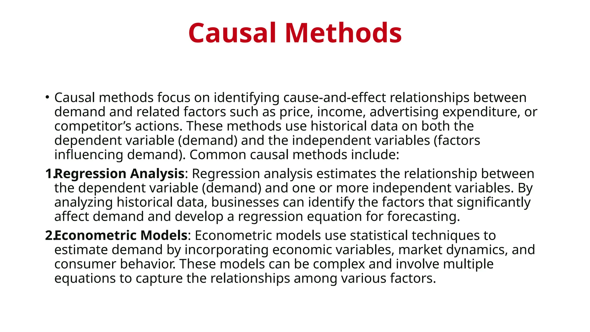
29. Causal Methods
• Causal methods focus on identifying cause-and-effect relationships between
demand and related factors such as price, income, advertising expenditure, or
competitor’s actions. These methods use historical data on both the
dependent variable (demand) and the independent variables (factors
influencing demand). Common causal methods include:
1.Regression Analysis: Regression analysis estimates the relationship between
the dependent variable (demand) and one or more independent variables. By
analyzing historical data, businesses can identify the factors that significantly
affect demand and develop a regression equation for forecasting.
2.Econometric Models: Econometric models use statistical techniques to
estimate demand by incorporating economic variables, market dynamics, and
consumer behavior. These models can be complex and involve multiple
equations to capture the relationships among various factors.

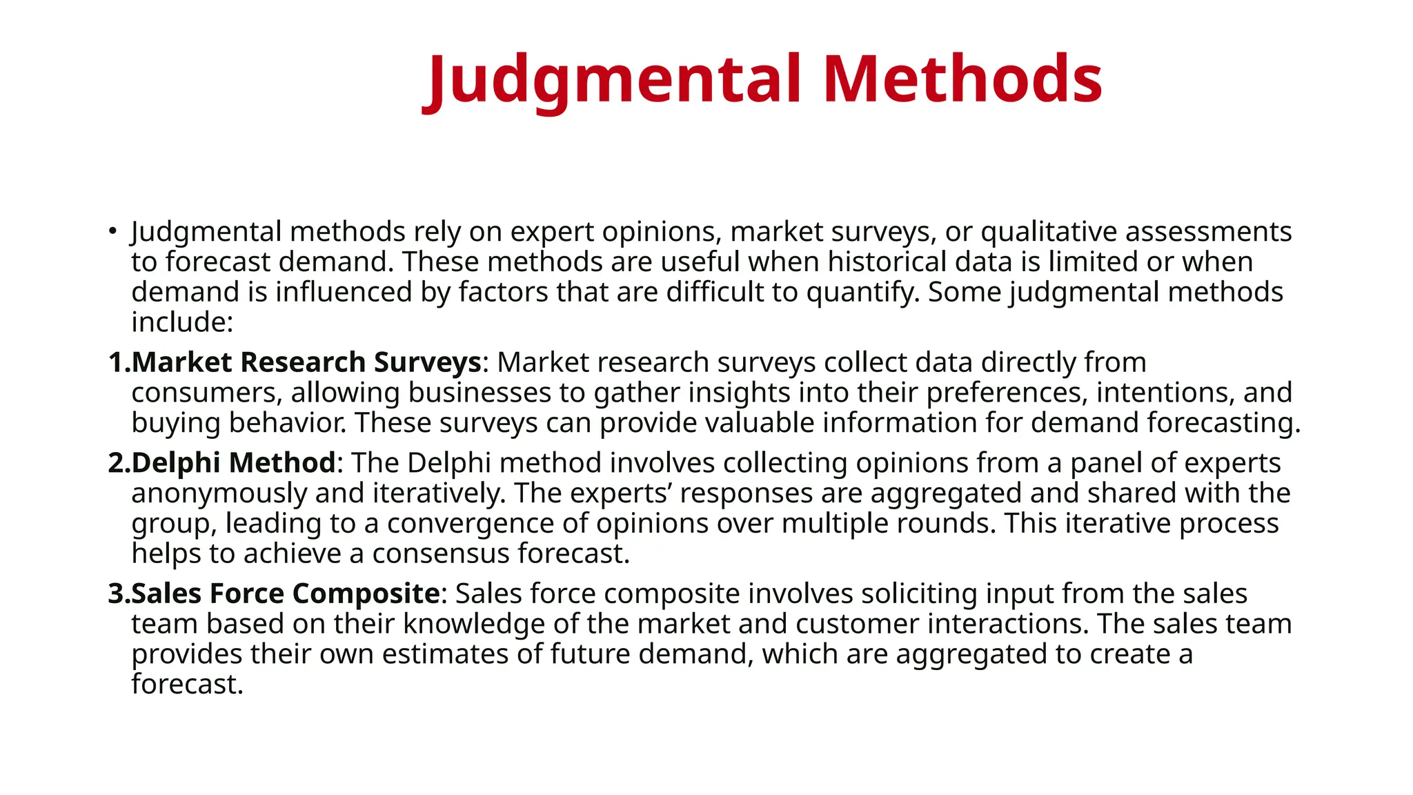
30. Judgmental Methods
• Judgmental methods rely on expert opinions, market surveys, or qualitative assessments
to forecast demand. These methods are useful when historical data is limited or when
demand is influenced by factors that are difficult to quantify. Some judgmental methods
include:
1.Market Research Surveys: Market research surveys collect data directly from
consumers, allowing businesses to gather insights into their preferences, intentions, and
buying behavior. These surveys can provide valuable information for demand forecasting.
2.Delphi Method: The Delphi method involves collecting opinions from a panel of experts
anonymously and iteratively. The experts’ responses are aggregated and shared with the
group, leading to a convergence of opinions over multiple rounds. This iterative process
helps to achieve a consensus forecast.
3.Sales Force Composite: Sales force composite involves soliciting input from the sales
team based on their knowledge of the market and customer interactions. The sales team
provides their own estimates of future demand, which are aggregated to create a
forecast.

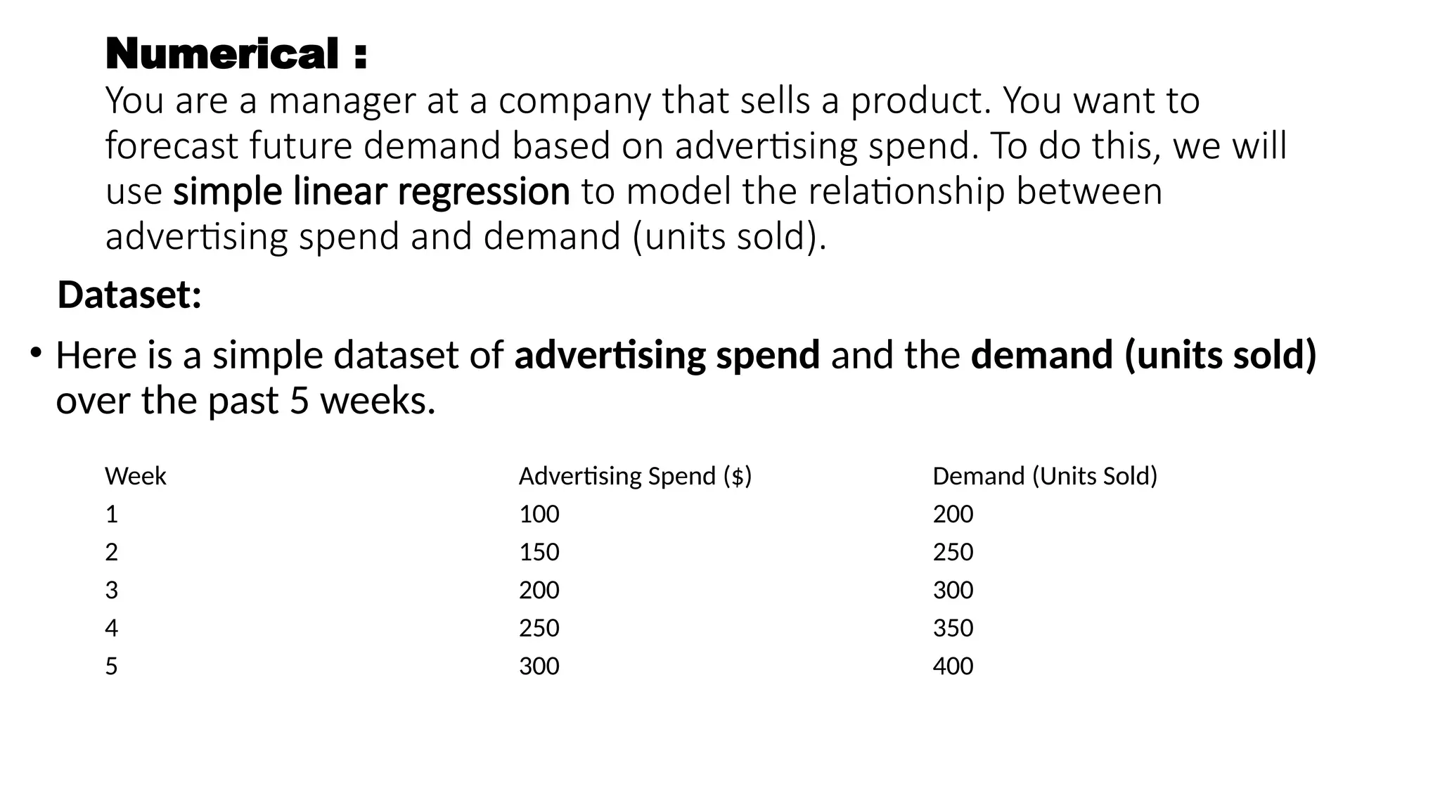
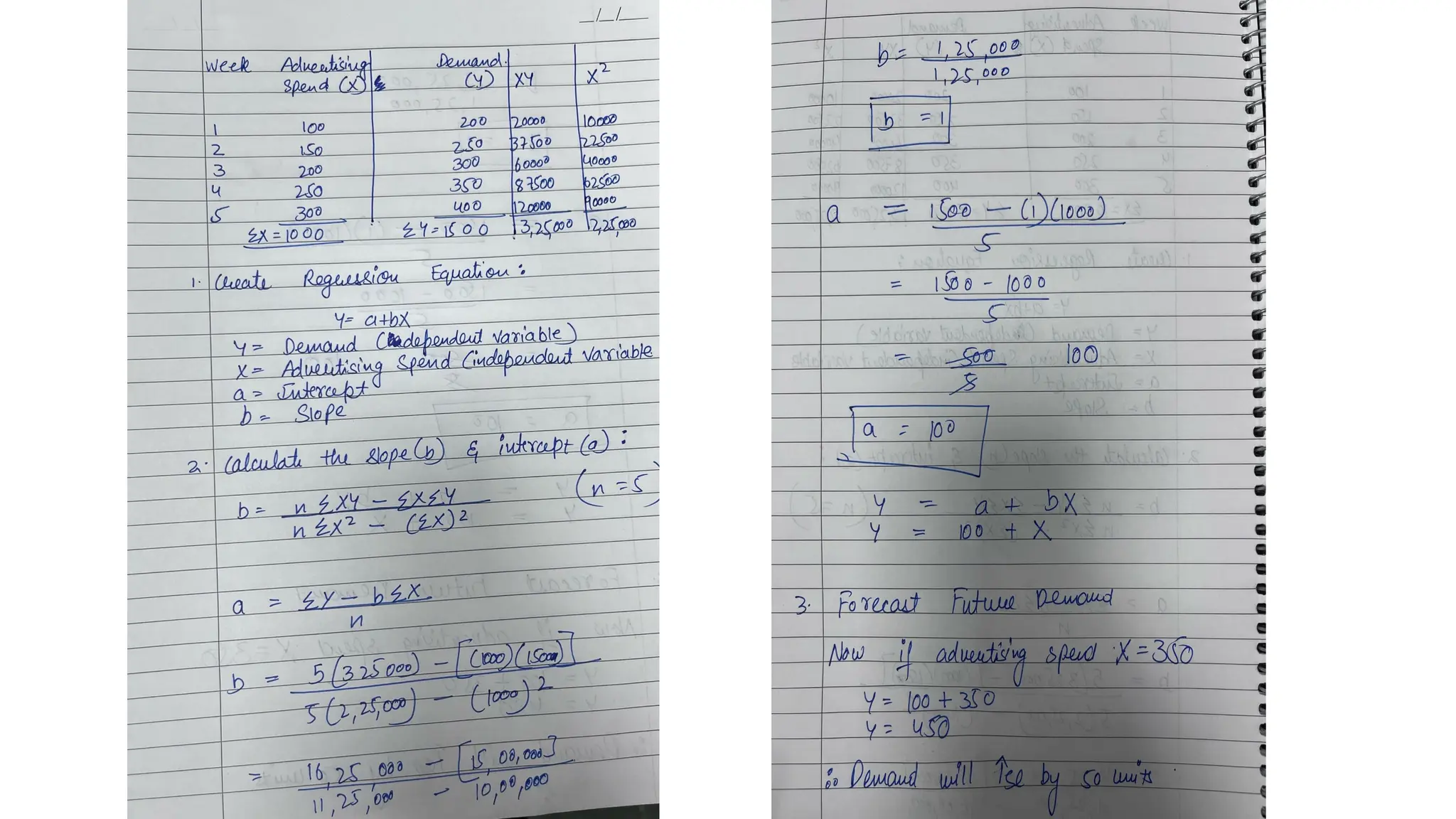
31. Numerical :
You are a manager at a company that sells a product. You want to
forecast future demand based on advertising spend. To do this, we will
use simple linear regression to model the relationship between
advertising spend and demand (units sold).
Dataset:
• Here is a simple dataset of advertising spend and the demand (units sold)
over the past 5 weeks.
Week Advertising Spend ($) Demand (Units Sold)
1 100 200
2 150 250
3 200 300
4 250 350
5 300 400

33. MEANING OF SUPPLY
Supply means the quantity offered for sale by producers at a particular
price.
Two important points are :– (i) Supply refers to what producers offer for
sale at a given price and
(ii) Supply is a flow concept. The quantity supplied is so much per unit
of time, per day, per week, per month or per year.

34. Determinants of Supply
I. Price of the good : Ceteris Paribus, the higher price of a good the greater the quantity of
it that will be produced and offered for sale.
II. Production technology : The supply of a particular commodity depends upon the state
of technology and changes in it. As technology progresses, it becomes possible to produce
commodities more cheaply.
III. Prices of factors : Another important factor which influences the supply of a
commodity is cost of inputs i.e prices of factors of production. Decrease in the prices of
these inputs makes it possible to produce commodities more cheaply.
IV. Prices of other commodities : The supply of a commodity depends not only on the
prices of the concerned commodity but also on the prices of other commodities. If the
price of a substitute goes up, firms will be tempted to divert their resources to the
production of that substitute. If price of a complementary product goes up, the supply of
the product in question also rises.

35. V. Objectives of the firm : Some firms want to maximise their profits. For that
they will produce and supply that much quantity which fetches maximum profits
to them. Some other firms may believe in lower margin and high sales turnover.
VI. Number of producers : If the number of firms is more, output also increases.
VII. Time : Supply is a function of time also. In the long run, it becomes possible
to overcome some constraints.
VIII. Govt. Policy : The govt. may levy taxes in the form of excise duty or sales tax
or import duty, or may grant subsidies. If tax is levied on a product, its cost of
production will go up and the quantity supplied will go down. Subsidies on the
other hand, reduce the cost of production and thus encourages the producers to
produce and sell more.
IX. Future price expectations : During inflation, sellers normally expect the
prices to rise further. Therefore, they will tend to hoard the commodity. This will
reduce supply and will cause its price to rise further.

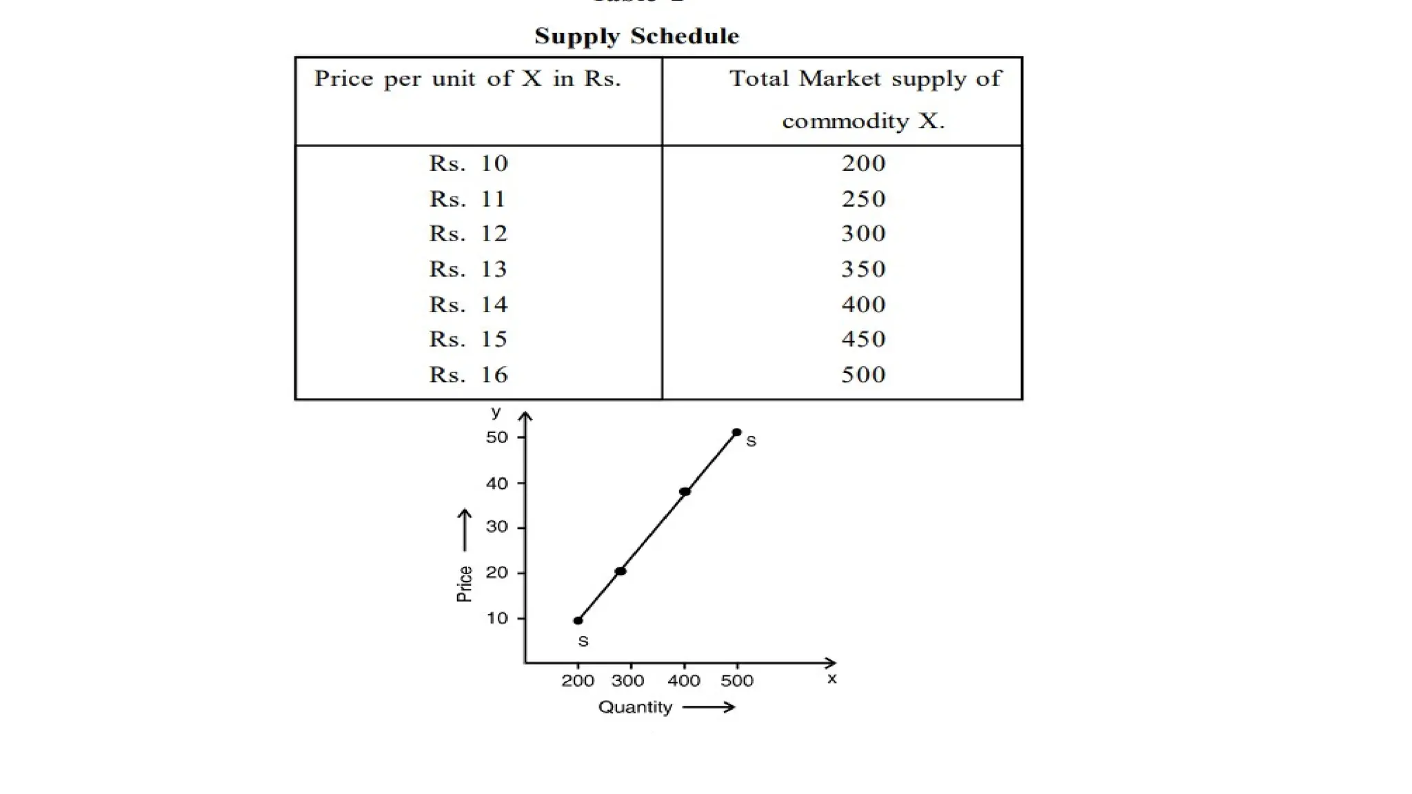
36. LAW OF SUPPLY
The law of supply explains the functional relationship between price
and quantity supplied According to this law, ceteris paribus, an increase
in price of a commodity causes an increase in its quantity supplied and
a decrease in its price causes its quantity supplied to fall. Thus, we find
a positive relationship between price and quantity supplied. It is based
on the fact that higher profits provide the producers an incentive to
produce more.
The law of supply can be explained through supply schedule and supply
curve given below :

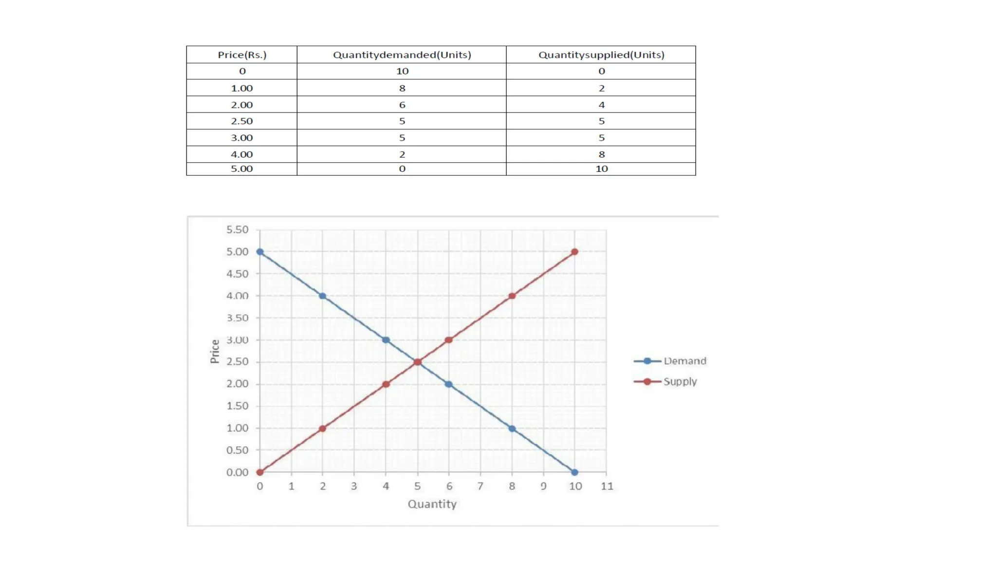
38. MARKET EQUILIBRIUM
• Market equilibrium refers to a situation where quantity demanded for a commodity is equals to quantity
supplied. We have seen that the demand and supply of any product depend on its price. The equilibrium price
is that price at which the total demand for any product in the market is equal to the total supply of that
product.
• The market demand curve gives us an idea of the total quantity demanded by all the buyers in the market at
different price levels. In the same way, each seller takes the price as given and decides to offer a certain
quantity for sale in the market. Thus, each seller has a n individual supply curve and by summing up the
individual supply curves of all the sellers in the market, we get the market supply curve. From the market
supply curve we get to know the total supply by all sellers at different prices.

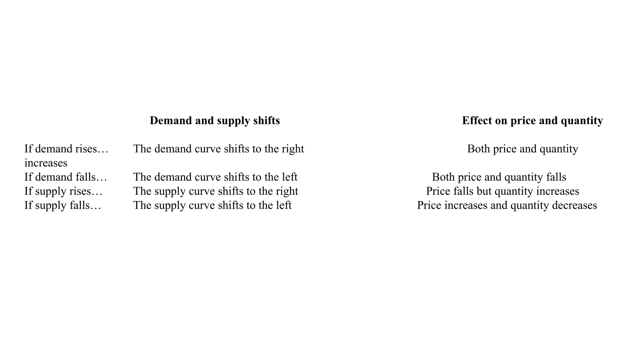
40. Demand and supply shifts Effect on price and quantity
If demand rises… The demand curve shifts to the right Both price and quantity
increases
If demand falls… The demand curve shifts to the left Both price and quantity falls
If supply rises… The supply curve shifts to the right Price falls but quantity increases
If supply falls… The supply curve shifts to the left Price increases and quantity decreases

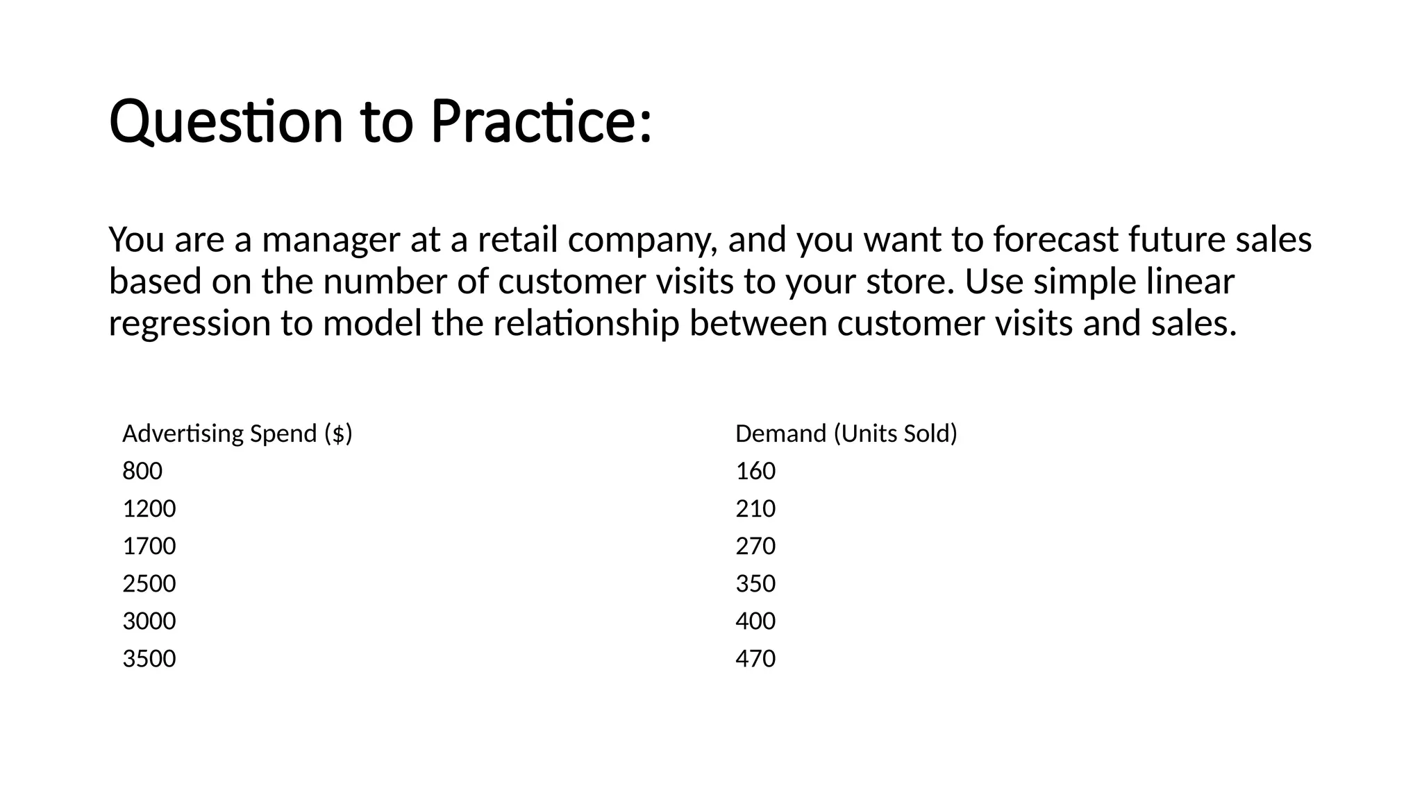
41. Question to Practice:
You are a manager at a retail company, and you want to forecast future sales
based on the number of customer visits to your store. Use simple linear
regression to model the relationship between customer visits and sales.
Advertising Spend ($) Demand (Units Sold)
800 160
1200 210
1700 270
2500 350
3000 400
3500 470