Thesis

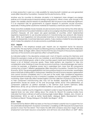
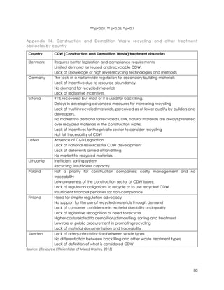
Analysis of the Effect the Adoption of
European Commission’s Set Targets for
Transition towards Circular Economy on
the Baltic Sea Region Countries
MASTER THESIS
GINTARE SKORUPSKAITE
2015
Thesis Supervisor: Christian Bjørnskov
Co-supervisor: Boris Georgiev

1
EXECUTIVE SUMMARY
During the writing of this paper, on the August 13th the world’s population reached its overshoot
day – the day, where, according to different measures, the total human consumption used up all
the natural resources the planet may replenish by itself in a year. The overshoot day has been
coming earlier and earlier each year since the start of this measurement in 1970.
Under the long term Europe’s plans for sustainable development the European Commission has
“intended to put the EU on course to using resources in a sustainable way” (European Commission,
Roadmap for moving to a low-carbon economy in 2050, 2015).
This paper was based on analysis of Resource Productivity (RP) as an indicator for economic
development in the light of European Commission’s commitment to embrace circular economy.
European Commission has identified that on the Business as Usual baseline, Resource Productivity
across EU would grow around 15% towards 2030, nevertheless indicates, that higher improvements
of 30% can be achieved with net positive impacts on total GDP (Economics, 2014) for EU28. In this
paper the focus will be on what the European Commission’s set target means on the macro-
regional level for the Baltic Sea Region1 and investigate how the move towards more circular
economy would benefit the Region.
The papers findings based on Environmental Kuznets Curve theory estimate that the Baltic Sea
Region as a whole will maintain increasing raw material consumption towards 2030 and will
experience a change only at the last years of investigation. A more rapid development of
resource productivity could speed up this turning point as well as significantly lower resource
consumption levels. The different countries of the BSR will experience very different growth patterns
and therefore require to adapt their policy focus respectively.
Estonia and Poland are predicted to have hard times ahead as their raw material consumption
little depends on the level of resource productivity. Germany, Finland, Sweden and Denmark are
underway in cutting their consumption levels, but more effort has to be put in as the European
proposed target of 2% annual increase will have little effect. On the other hand Lithuania and
Latvia will see rapid increase in their raw material consumption, but with increases in resource
productivity will be able to cap consumption and lower it to more sustainable levels going towards
2030.
The Baltic Sea Region countries need to put stronger effort in aiming policies to close resource
loops through further push for renewable energy, environmental tax reforms, elimination of
environmentally harmful subsidies and extended producer responsibility. A strong emphasis has to
be put on more sustainable use of non-metal ores in the industry sector as it is the leading factor
of high material consumption in the Baltic Sea Region, whilst with little current comprehensive
legislation. What is more, a better regional cooperation and interconnected infrastructure is
needed in the Baltic Sea Region to enhance future sustainable development.
1 Includes Denmark, Sweden, Norway, Finland, Estonia, Latvia, Lithuania, Poland and Germany.

2
TABLE OF CONTENTS
Executive Summary ..........................................................................................................................................1
Table of Figures..................................................................................................................................................3
1 Introduction ................................................................................................................................................5
1.1 Research relevance.........................................................................................................................5
1.2 Baltic Sea Region..............................................................................................................................7
1.3 Research Question...........................................................................................................................7
1.4 Delimitations ......................................................................................................................................8
1.5 Structure .............................................................................................................................................8
2 Theoretical Background...........................................................................................................................9
2.1 Kondratieff economic prosperity cycles......................................................................................9
2.2 Trade–off between Economic Growth and Environment ......................................................10
2.3 Resource Efficiency........................................................................................................................11
2.3.1 Decoupling..................................................................................................................................12
2.3.2 EU Initiatives .................................................................................................................................12
2.4 Circular Economy...........................................................................................................................12
2.5 Key Drivers of Resource Productivity...........................................................................................15
3 Research Methodology..........................................................................................................................16
3.1 Towards Circular Economy through resource productivity....................................................17
3.1.1 Defining Resource Productivity................................................................................................17
3.2 Literature review on model estimation.......................................................................................18
3.2.1 Regression model .......................................................................................................................20
3.2.2 Regression Variables..................................................................................................................21
3.3 Estimating Raw Material Consumption ......................................................................................22
3.4 Data ..................................................................................................................................................24
3.4.1 Raw Material Classification ......................................................................................................24
3.4.2 Estimating Raw Material Equivalent Coefficients ................................................................25
3.4.3 Data Quality................................................................................................................................25
4 Analysis ......................................................................................................................................................26
4.1 Global Resource Trends ................................................................................................................26
4.2 Resource use in the Baltic Sea Region .......................................................................................30
4.2.1 Resource Extraction ...................................................................................................................30
4.2.2 Trade Balance.............................................................................................................................31
4.2.3 Material Consumption...............................................................................................................33
4.3 Resource Productivity....................................................................................................................34

3
4.4 Discussion of the Resource Productivity measure....................................................................36
4.5 Empirical Evidence.........................................................................................................................38
5 Results.........................................................................................................................................................45
5.1 Towards 2030 ...................................................................................................................................45
5.2 Resource productivity gains.........................................................................................................47
5.3 Policy Implications to Support Circular Economy in the BSR..................................................49
5.3.1 Renewable Energy.....................................................................................................................49
5.3.2 Household Consumption ..........................................................................................................50
5.3.3 Imports..........................................................................................................................................52
5.3.4 Taxes .............................................................................................................................................52
5.3.5 Non-metal ores ...........................................................................................................................53
5.3.6 Discussion of the measures for resource productivity .........................................................55
6 Conclusions...............................................................................................................................................57
7 References................................................................................................................................................59
8 Enclosures..................................................................................................................................................66
TABLE OF FIGURES
Figure 1. Kondratieff Cycles – waves of prosperity.....................................................................................9
Figure 2. Resource, labor and capital productivity in EU (2000=100) ...................................................11
Figure 3. The biological and technical materials under circular economy. .......................................13
Figure 4. Overview of economic and environmental effect under circular economy ....................14
Figure 5. The Environmental Kuznets Curve................................................................................................15
Figure 6. Economy – wide material flow – based indicators ..................................................................18
Figure 7. Economy-Wide material balance scheme ...............................................................................22
Figure 8. Global extraction of material resources 1980-2007 .................................................................27
Figure 9. Global Commodity prices 2010 = 100, real 2010$ ....................................................................28
Figure 10. Resource Material Consumption in EU28 .................................................................................29
Figure 11. The difference between EU28 imports and exports measured in simple weight and in
RME for 2012 .....................................................................................................................................................29
Figure 12. Risks by Resource Category .......................................................................................................30
Figure 13. Material imports (left) and exports (right) in the Baltic Sea Region 2012..........................31
Figure 14. Trade Balance of the BSR measured in physical terms (figure a) and RME (figure b) 2002-
2012 by material category............................................................................................................................32
Figure 15. Domestic Extraction, Imports in RME and RMC in the BSR 2002-2012 by material category
............................................................................................................................................................................33
Figure 16. Total Raw Material Input (RMI) composition by country (2012) and material category34
Figure 17. GDP, RMC and RP change in the Baltic Sea Region 2002-2012 .........................................35
Figure 18. Resource Productivity by country 2012 ....................................................................................35
Figure 19. Comparison of RP measured in DMC and RMC for Baltic Sea Region..............................37
Figure 20. Growth in RMC/capita (y axis) and GDP/capita (x axis), 2002 -2012 ................................38

4
Figure 21. Raw material consumption per capita and GDP per capita relation...............................39
Figure 22. Estimation results from different regression models on GDP measures without Finland .39
Figure 23. Comparison of different model estimations............................................................................41
Figure 24. F-test on IV significant on GDP/cap and GDP/cap^2 measures .......................................42
Figure 25. Comparison of OLS, IV, Fixed Effects with IV (corrected for cluster robust errors) and Fixed
Effects (corrected for cluster robust errors)................................................................................................44
Figure 26. Baltic Sea Region raw material consumption towards 2030................................................46
Figure 27. Expected Renewable Energy levels in Member states compared to targets .................49
Figure 29. Key priorities for the BSR country policymakers for resource productivity.........................56

5
1 INTRODUCTION
The year 2015 is an important one for everyone at least a bit concerned with the environment and
climate change. Recognizing global warming as one of the most serious and complex challenges
facing humankind, this year's World Economic Forum meeting devoted 23 sessions to climate
change. In Europe, another problem, which raises concern is the continent’s dependency on
other countries for raw material imports and with increasing prices, this is causing added pressure
on the already weakened market. What is more, the growing global population predictions of
some 3 billion new consumers entering the middle class by 2030 raises deep concerns on the
efficient use of already scarce resources. As the industrial revolution mantra of “take-make-
consume and dispose” is not serving the needs of society anymore, there is a need for a new
approach, which would transform the linear use of our resources to a more sustainable one.
European Union has already recognized that through increased resource productivity, it can, not
only benefit the fragile state of the environment, but also positively contribute to the economic
growth of its Member States. It has recently set out targets for resource productivity as well as
municipal and packaging waste recycling (Commission, 2014). Just achieving the new waste
targets predicts 180 000 new jobs around the European Union and 72 billion Euro savings in waste
management costs (European Environmental Burreau, 2015).
This paper was based on analysis of Resource Productivity (RP) as an indicator for economic
development in the light of European Commission’s commitment to embrace circular economy2.
European Commission has identified that on the Business as Usual baseline, Resource Productivity
across EU would grow around 15% towards 2030, nevertheless indicates, that higher improvements
of 30% can be achieved with net positive impacts on total GDP (Economics, 2014) for EU28. In this
paper the focus will be on what the European Commission’s set target means on the macro-
regional level for the Baltic Sea Region3 and its underlying countries.
This section of the paper will briefly summarize the reason behind the carried out research, the
research questions raised, the topic’s relevance in today’s economic setting as well as the
delimitations of the paper.
1.1 RESEARCH RELEVANCE
The motivation for this research paper stems from the general concern on human based
economic activities and how they affect the environment. The previous century lifestyle of
consumption as the leading indicator for economic growth has led to quite staggering
consequences, which the current population is starting to feel.
For the past 10,000 years the Earth’s environment has been stable – known as the Holocene period.
Since the Industrial Revolution, a new era has arisen – the Anthropocene – where the
environmental changes are led not by natural swings, but enabled by human development. There
is a growing consensus that human led activities, heavy reliance on fossil fuels, industrialized
agriculture are a threat to the stability of the world’s ecosystem and could lead to a more unstable
2 http://ec.europa.eu/environment/circular-economy/
3 Includes Denmark, Sweden, Norway, Finland, Estonia, Latvia, Lithuania, Poland and Germany.

6
environment. Human based activities have already pushed through three planetary boundaries
and are approaching to surpass four more4.
There are few who are ignorant to the human induced climate change, which is affecting
everything from everyday lives, to how business is conducted. The terms “eco-friendly”, “green”,
“energy-efficient”, “sustainable” are becoming a must-be in many parts of the developed world.
The year 2015 is an important year for the future economic development, with many talks
happening on climate change and with the biggest focus this year with eyes on Paris in December
for Conference of Parties, 21st meeting, COP21. Given the subsequent meetings at Copenhagen
2009, Doha 2012, Warsaw 2013, and Lima 2014, the meeting in Paris at the end of this year will be
a significant one as the conference for the first time as its objective has put a goal of reaching a
legally binding universal agreement for fight against climate change and restricting global
warming below 2 degrees Celsius. Each country is obligated to take responsibility for combating
climate change and are expected to submit their Climate Action Plans prior the conference.
The European Union has submitted its Climate Action Plan already on the 6th March well in
advance with set targets to cut greenhouse gas emissions by 20% compared to 1990 level, have
20% of all energy consumption coming from renewable energy and a 20% increase in energy
efficiency by year 2020 (European Commission, 2015). This is in line with the EU Roadmap for
moving to a low-carbon economy in 2050, which is one of the long-term policy plans under the
Resource Efficient Europe Flagship initiative “intended to put the EU on course to using resources
in a sustainable way” (European Commission, Roadmap for moving to a low-carbon economy in
2050, 2015).
Under this flagship the EU has acknowledged the need to move towards a more circular economy
of closed loop production and consumption. It has measured that an improvement in resource
productivity could boost the total GPD by 2-3.3 %, create up to 2.6 million new jobs and reduce
the total resource use by 17 to 25% (compared to the business as usual) (Meyer, 2011). Due to the
high risks associated with resource use in Europe, this becomes an interesting aspect to observe
more closely. The European Commission’s paper nevertheless looked only at the effect on the
total EU27 based on resource productivity increases on 1, 2 to 3% per annum scenarios. This does
not show in what way countries in different economic states would be affected and would it make
sense for all countries to unanimously strive to implement the proposed target of resource
productivity improvement of 2% per annum leading to around 30% increase by 2030 (EUROPEAN
RESOURCE EFFICIENCY PLATFORM, 2012).
For this reason this paper will focus on looking at the suggested European Commission’s targets for
resource productivity in order to lower resource consumption and as its country base will choose
to look at the Baltic Sea Region countries. The main contribution of this paper will thus provide
insight how EU countries of different economic development should adapt their national policy
mixes and set individual objectives in order to strive towards a resource efficient region.
In order to explain the patterns of resource productivity and its impact on GDP growth, the
theoretical understanding of relationship between resource consumption and economic input is
needed. Here, a lack of historic analyses on resource consumption, results that no established
theoretical framework is available at the moment (Bleischwitz, Bahn-Walkowiak, Onischka, Röder,
& Steger, 2007). Nevertheless, most commonly seen approach in the studies of environmental and
economic links, is seen as the Environmental Kuznets Curve. The Environmental Kuznets curve has
44 See Appendix 1

7
been seldom used to measure resource use and focused mostly on different pollution measures,
therefore this paper gives a broader application of the theory in environmental economy.
1.2 BALTIC SEA REGION
The Baltic Sea Region (BSR) in itself is a good proxy to the different European countries due to its
diversity in country economic development, where you have the emerging high potential for
growth holding, yet small, Baltic countries on one side and the highly developed and
environmentally conscious Scandinavian countries on the other.
The Baltic Sea Region account for 85 million Europeans, which share similar features and
challenges. It is the first-macro region to have its own development strategy to enhance
cooperation, improve the condition of the Baltic Sea and increase prosperity (EU Strategy for the
Baltic Sea Region, n.d.). What is more, under the 2010 Vilnius Declaration, the “Vision for the Baltic
Sea Region by 2020” has put a strong focus on sustainable development in two major areas –
Climate Change adaptation and Green Economy. In the field of sustainable development, “the
Council calls on the Baltic Sea Region member states to become front runners in the development
and implementation of actions towards green economy and facilitate collaboration in this
respect and promote the incorporation of sustainable consumption and production instruments
in sectorial policies” (Council of the Baltic Sea States , 2014).
There is no scientific way to exactly determine the boundaries of the Baltic Sea Region. In different
sources it is represented with slight variations, mainly regarding Iceland and Norway, which
technically do not boarder with the Baltic Sea nevertheless due to their close co-operation with
the BSR countries are included in some sources. Also countries like Poland, Germany and Russia in
some cases are only partially included in the region’s definition as only some administrative areas
have a distinct connection to the Baltic Sea Region5. For the purpose of simplicity the boundaries
of the Baltic Sea Region will be defined as the simplified version of the definition used by the
Council of the Baltic Sea States (Baltic Development Forum, 2014). Therefore the countries of
interest are: Denmark, Estonia, Finland, Germany, Latvia, Lithuania, Poland and Sweden. Russia,
Norway and Iceland, although part of the Baltic Sea Region under the definition of CBSS, will be
excluded due to the fact that EU suggested targets and regulations do not apply to these
countries as they are not part of EU.
The different actors of the Baltic Sea Region – the Scandinavian countries, Germany, the Baltic
countries and Poland hold distinct differences both demographically, by ecological footprint as
well as economic growth. Due to these differences this paper gives a good opportunity to
observe what effect on resource consumption the proposed environmental targets have for
countries of different economic states.
1.3 RESEARCH QUESTION
In regards to the recent developments of the European Union for a more sustainable Europe, the
main problem statement of this paper thus becomes:
What effect on resource consumption the adoption of European Commission’s set target for
transition towards a more Circular Economy towards 2030 will have for the Baltic Sea Region
member countries and the Region as a whole?
5 (Baltic Development Forum, 2014)

8
In order to delve deeper into how countries may be able to reach the proposed targets
supplementary research questions will also cover:
 What influences resource productivity growth; as well as
 What policy implications can help stimulate resource productivity in the Baltic Sea
Region
1.4 DELIMITATIONS
This paper faces few key challenges, with most stemming from lack of studies yet available on
circular economy. The concept itself has only started to be adapted more thoroughly quite
recently, therefore there is no well-grounded framework set, mostly just individual country or
company initiatives are available.
The indicators that are used in this paper, although widely accepted by the Member States as
good indicators for resource consumption, lack country specific data as well as the ability to look
into resource consumption at a more disaggregated level.
Data on waste management has proven to be also widely scarce, which resulted in shortcomings
of this paper. Also, land use, water and air were not considered in the paper as part of resources.
During the forecast of future raw material consumption towards 2030 only GDP and Resource
Productivity have been used to derive the forecasts. Other variables proved to be hard to
estimate reliably. Dropping some of the significant variables, increase the power of GDP and RP,
which distorts the findings slightly. Nevertheless, such estimates prove to be rather difficult to carry
out in a reliant manner, but propose further possibilities to build on this model.
1.5 STRUCTURE
The paper is organized in 8 distinct sections. Section 1 serves as the introductory chapter of the
paper, briefly introducing the topic, reasoning for the relevance and summarizing the scope of
the paper. Section 2 invites the reader to get acknowledged with the theoretical background,
while section 3 introduces the research methodology. Based on these parts the following section
presents the analysis that has been conducted, where both descriptive and empirical studies are
represented. Section 5 summarizes the results for the previous analysis section, discusses the
findings and proposes policy implications based on the findings. Lastly, section 6 concludes the
overall paper, while sections 7 and 8 present the literature reference list and enclosures
respectively.

9
2 THEORETICAL BACKGROUND
2.1 KONDRATIEFF ECONOMIC PROSPERITY CYCLES
The world’s growing interconnectedness arising from the globalization is presenting both
opportunities and threats to the societies as already seen numerous times throughout history. The
stronger links and interdependence of economic, cultural, political, social dimensions have, in turn,
brought economic growth and prosperity, mobility, technology driven innovation and market
competition. But through this diminishing importance of distance, the world has also experienced
how economic downturns, happening in other parts of the world, still have a huge effect world-
wide, exactly because of this inter-connectedness – most recent and biggest one, being the
financial crisis of 2007.
These kind of economic ups and downs can be seen all throughout the industrial times. There have
been 5 distinct major waves documented in the past 200 years, commonly known as the
Kondratieff waves, or cycles and there is a rising discussion whether the recent economic crisis
could have marked the start of the new, sixth K – cycle. According to the studies of the Russian
economic Nikolai Kondratieff on economic cycles, each cycle has distinct features as starting
with new factors of production and innovation, triggering economic growth.
Figure 1. Kondratieff Cycles – waves of prosperity
Source: (Allianz Global Investors, 2010)
In the process (Wilenius, 2014):
• New industries arise,
• Changes in corporate structures arise,
• New professions emerge,
• Economic growth is observed, typically associated with rising equity markets.

10
Each new technological upbringing nevertheless, at some point reaches an exhaust of basic
innovation, secondly, it is possible to observe an excessive amount of capital compared to
physical capital, which, thirdly, triggers “a passage of severe recession, a gateway for radical
change. And fourthly, surplus of institutional and social changes occur, leading to new
organizational cultures” (Wilenius, 2014). Each of these stages arguably have been observed in
the recent financial crisis, marking the transition period into the 6th Kondratieff cycle (Allianz Global
Investors, 2010).
If the previous growth period was mainly driven by the ICT sector technological innovations, the
upcoming period megatrends are indicated to be led by environmental technologies coupled
with health sector expansion (Wilenius, 2014), (Allianz Global Investors, 2010). The new K – cycle
will be mainly driven by the demographic changes in aging population of the developed world,
growing economic status of the emerging population (China and India) together with the setting
concerns on resource scarcity and climate change. “This makes the environmental market a hot
candidate for a major role in the 6th Kondratieff cycle.” (Allianz Global Investors, 2010).
2.2 TRADE–OFF BETWEEN ECONOMIC GROWTH AND ENVIRONMENT
This new wave also brings a new understanding on the societal level of the responsibilities
attached to human activity. This societal change has been not as radical throughout the previous
waves as the technological changes. Since the industrial revolution, consumerism has been the
leading organizing principle of modern life, feeding back into the need for further industrialization
and technological development (Commodities, Consumerism & Industrialization). The
environmental consequences arising from the industrialized economies are not evident straight
away; residues, toxic waste take time to accumulate before they start to make significant harm
to living organisms. The Earth Summit in Rio 1992 in its meeting concluded that the economic,
social and environmental problems are inescapably linked to the world development and vice
versa. And the social and economic welfare of human beings depend on this linkage as well
(Awan, 2013).
There is a trade-off between economic growth and the environment, because of the excessive
use of available resources on the expense of environmental externalities. For this reason it can be
observed that the most pollution is created in the developed world and not the poorer countries
(EPA). United States holds only 2% of the world’s population, nevertheless contributes for almost
25% of the world’s pollution, Europe follows a similar tendency (Awan, 2013).
As income and consumption increases, so does the strain on the environment to replenish the
used resources and to accumulate the waste. It would be inhumane to deny poorer countries
access to higher welfare as well as it would be impossible to stop the economic growth in the
developed world. Also, through the already mentioned globalization factors, the growth in the
poorer countries is interlinked with the economic state of the rest of the world as they are
dependent on the technology and knowledge transferred to them (Patel, 2008). Therefore it is the
responsibility of the developed world to lead the sustainable growth model through
environmentally sound technology, which could be transferred to the developing countries. “But
the growth models of industrial nations must change drastically. The current quantity of growth
should be replaced by quality” (Awan, 2013). Technological developments need to lead to further
growth without the use of more resources, therefore sustainable in the long run.

11
2.3 RESOURCE EFFICIENCY
As natural resources make up the fundamental base for economic growth, they are an important
part of any society. The processes for extraction, processing, refinery and use are all important
undertakings and sources of economic activity in many countries.
Resources can take up different forms (Service, 2011):
 Raw materials
 Flow resources (wind, solar, tidal of geothermal energy)
 Land
 Environmental medium ( such as air, soil and water)
The economy can grow by being driven by demand for production. As production requires input,
the demand for input is also growing, therefore if wanting to maintain economic growth the
factors of input have to be addressed. In the case where input is finite and growing scarcer, this
puts pressure on the industry to use the materials in the best way, cut waste – become more
efficient. Resource efficiency addresses the notion on how to “produce more with less“.
Technological improvements can be seen throughout history in how they affected the both use
of material resources and labor. Labor productivity, though has seen a lot higher increase
compared to resources, mainly driven by incentives formalized by increasing labor costs much
faster than material costs. Frankly, there was lack of incentive to try to increase efficient use of
resources. Literature suggests (SERI, 2013), that labor productivity has already increased to the
point, where further increases start to negatively impact the quality of output and results in
different negative effects (work depression, burn-out). On the other hand, resource productivity
has not yet been explored to its fullest. The recent financial crisis has been a good example of this
as illustrated in the figure below, during which, companies were faced by the necessity to increase
their resource productivity in order to stay in business, managing to increase their efficient product
use in relatively short time.
Figure 2. Resource, labor and capital productivity in EU (2000=100)
Source: (SERI, 2013)

12
2.3.1 Decoupling
“Resource decoupling means reducing the rate of use of (primary) resources per unit of
economic activity. This ‘dematerialization’ is based on using less material, energy, water and land
resources for the same economic output. Resource decoupling leads to an increase in the
efficiency with which resources are used.” (l. Fischer-Kowalski, 2011). Increasing recourse
productivity has already resulted in some relative decoupling from economic growth, nevertheless,
mainly in the developed countries (OECD, Resource Productivity in G8 and the OECD, 2008).
Nevertheless, relative decoupling cannot be sustainable in the long run as it just indicates that the
negative externalities related to resource use and extraction are growing in a slower pace than
economic welfare. It is, yet, still growing. Therefore it is necessary to try to drive absolute
decoupling – declining environmental impact, while increasing economic growth.
2.3.2 EU Initiatives
The EU is quite an open economy in terms of trade and one of the main reasons for this is its high
dependency of material input for industrial production. EU has by far one of the highest
dependency rates for the majority of material and energy sources in the world. According to 2000
data, EU-25 has had a ratio of 21,5% or resource dependency (physical trade balance divided by
the domestically extracted materials) – higher than any other region (Elkins, 2009). This means that
a lot of the environmental pressure associated with resource material extraction is outsourced
from EU to the other countries yet leaves EU heavily dependent on them for imports. This creates
a potential risk problem for resource security, especially with the growing demands for raw
materials of China and other fast emerging countries.
EU has already taken steps to address this issue, together with environmental and resource
productivity related concerns through, to name a few, the Raw Materials Initiative, creating an
Energy Union (European Commission, Energy Union, 2015), EU-USA Free Trade Agreement
(European Commission, EU-US Free Trade Agreement, 2015), deepening the Single Market for
goods and services (European Cmmission, 2014), A resource-efficient Europe – Flagship initiative
under the Europe 2020 Strategy (European Commission, A resource-efficient Europe – Flagship
initiative under the Europe 2020 Strategy, 2011) under which one of the key measures for creating
a resource-efficient marketplace is the move towards circular economy in EU.
2.4 CIRCULAR ECONOMY
The different concepts surrounding environmental impact are not new; “sustainable
development”, “zero-waste”, “low-carbon economy” are concepts that have been present for
some time. Nevertheless, the global trends in resource use, the growing concerns for climate
change and the growing risks associated with resource dependency has stimulated the need to
re-think the “take-make-consume and dispose” pattern of consumption. It is also taking up a
higher level of the 3 R’s (Reduce, Re-use and Recycle”) (Eisenberg, 2008). It is not enough only to
use less, waste less, minimize environmental impact and cut down on emissions. There is a growing
understanding that in order to reverse the damages already inflicted on the environment, it is not
enough to be more efficient in doing business in the old way, or being “less bad”, less polluting
(but polluting nonetheless); there is a need to re-think how business is conducted in general as the
mere reduction of resources used, will not alter the finite nature of their stocks. A change of
understanding of the entire operating system seems to be in need.
Therefore, already in 2012, following after the financial crisis and the inability to regain strength in
the global context, EU has adopted the manifesto striving for a resource- efficient Europe, under
which the move towards circular economy has become its essential part. “In a world with growing

13
pressures on resources and the environment, the EU has no choice but to go for the transition to a
resource-efficient and ultimately regenerative circular economy.” (European Commission,
Manifesto for a resource-efficient Europe, 2012).
Circular Economy:
 Is a global economic model that decouples economic growth and development from the
consumption of finite resources in absolute terms;
 Distinguishes between and separates technical and biological materials
 Focuses on effective design and optimal use of materials
 Provides new opportunities for innovation across different fields
 Establishes a framework for a resilient system able to work in the longer term (The Circular
Model - an overview, 2013)
Circular economy is a regenerative model by intention. At the core of its concept is production
for disassembly; “waste does not exist” (Ellen MacArthur Foundation, 2014), where the close
product cycles are designed to enter the use-cycle once their current life-cycle is over.
Figure 3. The biological and technical materials under circular economy.
Source: (Ellen MacArthur Foundation, 2014)

14
Secondly, the model introduces the differentiation between two distinct product groups –
between consumable and durable components, where the consumables are mainly viewed as
the biological input (f.x. food, wood or cotton), or “nutrients”, which can most of the time be safely
returned into the biosphere. The durable components, such as technological outputs, plastics and
machines cannot be safely returned into the biosphere without significant damage, therefore
they, under circular economy, have to be designed from the start with the idea of disassembly,
to be able to come back into the use-cycle. These kind of materials have been coined as
“technological nutrients” by William McDonough and Michael Braungart in their book “Cradle to
Cradle: Remaking the Way we Make things” (McDonough & Braungart, 2002).
Circular economy thus provides many possibilities for companies to cut costs by limiting the need
for raw material input. Nevertheless requires disruptive and radical changes in the understanding
of linkages the product goes through in its value chain. Accenture has distinguished four main
areas of value creation in the circular economy (Accenture, 2014):
 Lasting Resources – that can be continuously regenerated
 Liquid markets – where products and assets are optimally utilized and widely accessible to
everyone
 Long Life cycles – where products are made to last
 Linked value chains – closed loop life cycles that result in no waste
Through repair and maintenance, reuse, remanufacture and refurbishment, the products are
aimed to be kept in use for as long as possible in order to extract the most value out of them. In
general, it is similar to thinking of cutting down a tree. It may be cut down and burned straight
away to produce heat. Or alternatively, it may be used to make a table, after that it may be
turned into chipboard, which at the end of its useful life can be then turned into particle board,
which afterwards can go through a digester to be returned into the biosphere. Under Circular
economy the product disposal through landfilling or incineration is the last step, which should be
avoided and discouraged to the point where the product has served to all its possibilities. This in a
long term will lead to future waste elimination.
Figure 4. Overview of economic and environmental effect under circular economy
Source: Based on (Ellen MacArthur Foundation, 2014)
CircularEconomy
Production for
disassembly
Resource Productivity
Increase economic
welfare
Create jobs
Reduce polution &
negative
environmental impact
Eliminate waste
Increase
competitivenes
Reduce resource
dependency
Renewable Energy

15
Circular economy should not be confused with perpetuity. Energy is still needed in the different
phases of both biological and technological materials. Under circular economy, the third
distinctive point, therefore, becomes the use of renewable energy sources for driving the
economy.
It is evident (see figure above) that circular economy is able to provide economic and social
benefits. A number of individual firms have already started to embrace the transition and are
seeing the effect it has on their business (Renault, Unilever, Phillips, etc.) (Ellen MacArthur
Foundation, 2014), but in order to increase the effect globally, nation-wide actions have to take
place, governments need to impose national strategies and policies to create a transparent
framework for companies to follow (UNFCCC, 2015).
In the past years, there have been attempts to quantify the effects circular economy may bring
globally (Ellen MacArthur Foundation, 2014), (World Economic Forum, 2012) and regionally
(European Commission, Towards a Circular Economy: A zero waste programme for Europe, 2014),
(Government of Netherlands, 2013), often with highly different results. This is due to the fact that
the notion of circular economy, even though not completely new, is still quite loosely defined,
therefore findings heavily depend on the research definitions, delimitations and used analytical
framework (Accenture, 2014). Below, the research methodology used for this paper will be
discussed and explained.
2.5 KEY DRIVERS OF RESOURCE PRODUCTIVITY
In order to be able to adequately explain the patterns of resource productivity and its impact on
GDP growth, the understanding of relationship between resource consumption and economic
input as well as the choice of relevant variables is essential. Here, a lack of historic analyses on
resource consumption, though results that no established theoretical framework is available at the
moment (Bleischwitz, Bahn-Walkowiak, Onischka, Röder, & Steger, 2007). Nevertheless, one most
commonly seen approach in the studies of environmental and economic links, is the use of
Environmental Kuznets Curve. The Environmental Kuznets Curve (EKC) follows the hypothesis of
inverse U-shape relationship between environmental quality and economic development; as
country economic welfare increases, so does environmental pressures up to a certain point upon
which the environmental pressures start to decline whilst economic welfare increase further (Stern,
2003).
Figure 5. The Environmental Kuznets Curve
Source: (Panayotou, 1999)

16
The EKC hypothesis arose in the early 1990s with Grossman and Krueger’s studies on world
development, nevertheless up till now still lacks empirical evidence for the different environmental
pollutants. The initial relationship stemmed from Simon Kuznets, who in 1950s has observed a similar
relationship between income and inequality, and the relation has been adapted to analyze
environment. Different studies report varied results based on the pollutant under investigation;
there has been positive relations found for some air pollutants, nevertheless results from studies on
water pollution are mixed, whereas there is little evidence to support the hypothesis for other
pollutants such as CO2 (Yandle, Vijayaraghavan, & Bhattarai, 2002) (Cialani, 2007).
Nevertheless, the hypothesis suggest few key important aspects to take in mind – firstly, that growth
in economic welfare will inevitably result in some environmental degradation, especially in the
high paced development stages, and secondly that further economic growth will help to offset
the previous environmental damage. This line of thinking is mainly based on the example of the
developed countries following their path of development from agricultural times to industrial
revolution and to the environment – conscious society that it is becoming today. Of course,
economic growth in itself is not enough to drive this change and other factors are important
(Dinda, 2004):
Technological change. New products, better technologies are more environmentally friendly and
efficient as also based on the Moore’s law of technological development. The technological
progress also makes better use of substitutive materials as to minimize the use of scares resources.
Change driven by structural demand. As the society progresses economically its preferences for
environmentally sound production also shifts. A more environmentally conscious society demands
better use, production and disposal of products, better quality water, air and soil. What is more,
de-industrialization and move towards more service driven economy will also influence resource
consumption.
Economic growth and saturation effect. As the economies progress, their development tends to
concentrate if large economical hub points, therefore the demand for infrastructural
development decreases over time benefiting from the condensation of economic activities at
one area. The level of environmental pollution gradually will start to decrease only at a point
where a certain economic development threshold is reached. Up to then, economic
development will be leading to more pollution.
It is questionable here, though, whether the differences between the two asserted country blocks
analyzed in this paper will be enough to identify that there is a significant inverted U shape relation
between resource consumption and economic output or whether the countries will present to be
already over the peak threshold and present only negative relationship. That is, of course, if the
relation between resource consumption and income will be present at all.
3 RESEARCH METHODOLOGY
This section will introduce the key determinants in analyzing the effect of the European
Commission’s proposed targets for resource productivity in regards to moving towards a circular
economy. In first, the different measures of resource productivity will be overlooked, discussing
some of the most recent studies on resource productivity. The key points for reference here will
mainly be the work of European Commission Analysis of EU target for Resource productivity and
related work.

17
3.1 TOWARDS CIRCULAR ECONOMY THROUGH RESOURCE PRODUCTIVITY
From the discussion above it has been identified that resource productivity is only one part
distinguishing circular economy and capturing its essence. Benefits from circular economy come
not only from increased resource productivity, but also from tracking of products, components
and materials (World Economic Forum, Towards the Circular Economy: Accelerating the Scale-up
accross global supply chains, 2014). What is more, the benefits of circular material use is distorted
if the energy used for this comes from fossil fuels. Therefore all parts of circular economy should be
addressed.
It is hard to address the component traceability as well as production for disassembly by empirical
studies. Nevertheless, calculating resource efficiency provides a quantifiable measure of circular
economy, as, “if the ultimate goal is to decouple economic growth from raw material use, then
the European Union’s Resource Productivity indicator is a strong contender” (Resource Event,
2015). As the aim of this paper is to analyze the effectiveness of European Commission’s proposed
target for Resource Productivity as an indicator for transition towards circular economy, this
measure will be deemed sufficient.
3.1.1 Defining Resource Productivity
Measuring resource productivity does not always have a direct path. Here it is important to express
resources in both their physical units (tones, kilograms, joules) as well as monetary equivalents to
show their economic value. It is quite widely accepted to use GDP as a measure for country
economic activity, although there has been also critics for the use of GDP for its lack of ability to
capture the quality of life and other aspects of human activities. By nature, GDP has been created
to measure only the monetary values of economic output related to production of goods and
services, therefore misses out on some of the aspects, like welfare and environmental well-being
(Costanza, Hart, Posner, & Talberth, 2009). Some of the criticisms pointed towards the use of GDP
focused on its measure of quantity and not quality of economic welfare. Nevertheless, as in this
paper the main focus is on resource productivity, thus on economic production of goods and
services, the GDP measure is sufficient for the purpose.
On the other hand, regarding material consumption, there is no consensus on the best indicator
to be used. Eurostat provides data for each country on their resource productivity based on
calculations on GDP and Domestic Material Consumption (DMC). European Commission has
identified, that the use of DMC, has significant drawbacks, as it does not take into account the
materials, which are produced in outside countries, therefore ignores the more international
dimension of material consumption (Commission, Analysis of EU Target for Resource Productivity,
2014). In other sources, the use of Total Material Requirement (TMR) or Total Material Consumption
(TMC) is used as, they consider all the material extracted, even those that do not physically enter
into the economy. Nevertheless, Eurostat does not provide data for neither TMC nor TMR and
would have to be estimated based on other given input. Another indicator, that could be used,
and, which is used by the European Commission is the Raw Material Consumption, which similar
to TMC accounts for raw material extraction abroad as if it would have been produced
domestically.

18
Figure 6. Economy – wide material flow – based indicators
Source: (SERI, Economy-wide material flow-based indicators, n.d.)
Both measures would require an estimation and in this case TMR may be viewed as an even further
extension of RMC. In that sense it should be possible to calculate TMR by multiplying RME by a
factor of total and unused material, nevertheless that would raise further problems. The unused
extraction data is relatively scarce, especially in metals (Karl Schoer, 2012), which would
complicate the estimate. For this reason Raw Material Consumption (RMC) will be chosen for its
proven ability to provide adequate measures as indicated by the studies of European Commission
(European Commission, Study on modelling of the economic and environmental impacts of raw
material consumption, 2014).
The Raw Material Consumption indicator represents the BSR countries in the global context as well
as let’s closely monitor the move towards “circular economy as increased recycling will lead to
less primary demand, and so, reduced RMC” (Commission, Analysis of EU Target for Resource
Productivity, 2014).
Calculating Resource Productivity (RP):
RP = GDP/RMC
Raw material consumption data does not exist on country level, only for the total EU as calculated
by Eurostat. It is currently working on producing estimates on the country-level, nevertheless for
the time being the RMC will have to be estimated manually. The European Commission’s study
using E3EM model provided by Cambridge Econometrics6 will provide the basis for estimation.
3.2 LITERATURE REVIEW ON MODEL ESTIMATION
In most EKC studies, longitudinal, or time-series cross sectional data (TSCS) has been explored
mostly by analyzing cross country data over a series of years. This is done in order to increase the
6 http://ec.europa.eu/environment/enveco/resource_efficiency/pdf/RMC.pdf

19
number of observations and deal with some of the shortcomings of using just cross sectional or
time-series data. As mentioned, this helps to increase the sample size as well as let’s capture
variation occurring from changes in both space and time simultaneously (Podesta, 2000)
Using TSCS data though, presents some difficulties of its own as it is subject to three main ordinary
least squares (OLS) assumption violations – serial correlation, contemporaneous correlation and
heteroscedasticity (Greene, 2000). Serial correlation violation occurs when the errors are
dependent from one time period to another, while contemporaneous correlation occurs when
the errors are affected similarly between observations, due to some external common shock.
Heteroscedasticity occurs when the errors are not similar and have different variances across units.
If these violations are present, then a linear OLS may not be the best estimator. For example, to
convincingly argue that cross country studies are spatially uncorrelated would be hard as to
ignore the many studies on social learning, herd behavior and neighborhood effects, which show
the presence of mutual dependence (Dukker, 2003). In his paper Dukker also argues that:
“because social norms and psychological behavior patterns typically enter panel regressions as
unobservable common factors, complex forms of spatial and temporal dependence may even
arise when the cross-sectional units have been randomly and independently sampled” (Dukker,
2003). He also argues that the standard error estimates for standard OLS or clustered standard
errors are biased, and therefore statistical implication is invalid.
There are two types of panel data, fixed and random effects. The fixed effects model explores the
relationship between the predictor and outcome variables within an entity, where each entity has
its own characteristics that could influence the estimation outcomes. The fixed effects model lets
control for the bias which comes from entity specific characteristics, which do not change over
time. Another important aspect here, is the assumption that the time invariant characteristics are
unique to each entity, therefore their error term and constant should not be correlated. If the errors
terms are correlated, that means random effects model is more appropriate, which allows for this
kind of correlation.
The brief summary of the assumptions required to be true under random effects can be
summarized as follows: (1) the entity specific effect is random and in uncorrelated with the
explanatory variables, (2) it assumes constant variance of the entity specific effect, (3) that all
repressors are not perfectly collinear. The first assumption is almost always hard to hold true,
therefore fixed effects most of the time seems more convincing. Fixed effects model lets in a
sophisticated way deal with the problem of omitted variables bias, nevertheless, one cannot
estimate the effect of time invariant explanatory variables which are observable. What is more,
this does not help solve the problem if the omitted variables do not vary over time. Here more
sophisticated modeling is required. What is more, the estimated parameters are conditional of the
country and time effects in the selected sample. Therefore the findings cannot be used to make
assumptions for other samples. In this case, it would not be right to use the data found for the
countries under investigation to make conclusions on other country consumption. In studies on the
Environmental Kuznets curve, most researchers have tried both random and fixed effects, where
fixed effects were more preferred under computing Hausman statistic to determine whether there
is correlation present between the explanatory variables and the errors term, but few have tried
to find out, why is this the case (Stern, Environmental Kuznets Curve, 2004). What is more, as
Podesta has argued, in many cases under political economy models “the issue created becomes
fixed effects vs no fixed effects, and not fixed effects vs random effects” (Podesta, 2000). This is
especially true when the variables change very slowly over time, therefore are highly collinear.

20
One way to deal with the arising problems has been suggested by Driscoll and Kraay by using
proposed standard error corrections that are robust in general forms of time and space
dependence. The method is argued to be superior over the more common used methods to
account for heteroscedasticity developed by White (1980), Huber (1967) or Newey and West
(1987) as it takes into account cross sectional correlation. For one thing, the model works
sufficiently well even with unbalanced panels as well as allows the error term to be autocorrelated,
heteroscedastic and cross-sectional dependent. It produces standard errors with are both
consistent and efficient. It deals with autocorrelation by introducing a time lag to which the
residuals are influenced. Under Monte Carlos simulations Hoechle (2007)shows that the Driscoll
and Kraay method tends to outperform pooled OLS estimate, when cross sectional dependence
is present regardless of the time spans. The pooled OLS tends to overstate the actual information
when the subjects are mutually dependent.
Another proposed model to account for the probable arising issues is proposed by Beck and Katz
(1995) by using OLS coefficient estimates with panel-corrected standard errors (PCSEs). The model
takes into account heteroscedasticity as well as any contemporaneous correlation of the errors.
However the model is still subject to serial correlation, which could be modeled out by including
a time lagged dependent variable together with other independent variables. Beck and Katz
argue that including such variable would let the statistician stay closer to the original data than
through transformation (Podesta, 2000). Nevertheless it should be accounted that the inclusion of
such variable usually leads to other variables loosing most of their explanatory power as most of
the variance becomes explained by the previous time period (Beurskens & Hekkenberg, 2011).
In the presence of few and not all violations, such as in the presence of heteroscedasticity and
serial correlation, but no contemporaneous correlation, OLS is still unbiased, but not efficient.
Neither are the standard errors. Nevertheless, fixes under these violations are simpler, as the
heteroscedasticity can be dealt with White’s robust standard error approach, which has been
long since documented and tested for its validity (White, 1980). Roger’s robust standard errors
account also for any serial correlation as well as heteroscedasticity. It can be used both in panel
data with fixed and random effects.
What is more, it is very feasible to believe that the model may suffer from endogeneity problem
as also suggested by other researchers (Lin, Paudel, & Pandit) as well as (Lin & Liscow). The
endogeneity problem may arise from different matters; measurement errors, simultaneity
problems or omitted variable bias. In the fact that there is still yet little data on the application of
Kuznets curve for environmental studies, and even more so, for resource consumption, the
problem has been little addressed before. It is very likely that there are unobserved factors that
affect income and consumption simultaneously. As there is reason to believe that the financial
crisis has had a meaningful impact on raw material consumption, it is obvious that the same shock
to the economy effected GDP as well. By this, it can be expected that OLS will yield inconsistent
results of any regression. What is more, even though the relationship that is being investigated here
is what effect increase in welfare has on raw material consumption, but what secures from that
the factors have a reverse effect as well, meaning, that an increase in material consumption has
an effect on the welfare itself as it stimulates material abundancy. This reverse causality would
pose the same inconsistent estimates under OLS. Taking into consideration possible endogeneity,
the use of Instrumental variables may be applicable.
3.2.1 Regression model
In regards to the data used in this paper, it is feasible to expect that the simple OLS model will be
subject to the aforementioned violations. It can be expected that serial correlation will be present

21
as, of course, the size of one year’s GDP will inevitably affect the size of GDP in the year to come,
as well as contemporaneous correlation will take effect as it is feasible to believe that all countries
have been effected by an external common shock – i.e. the financial crisis. Therefore the equation
used will be tested against the different proposed model options in order to production efficient
and consistent estimates.
As the EKC model proposes an inverted U shape relationship between the dependent and
independent variables, the quadratic function of the economic income will be taken into
account, nevertheless other relations, like linear and logarithmic will also be tested against the
quadratic form. So the following equations will be estimated:
𝑅𝑀𝐶𝑖𝑡 = 𝛽0 + 𝛽1 𝐺𝐷𝑃𝑖𝑡 + 𝑒𝑖𝑡
𝑅𝑀𝐶𝑖𝑡 = 𝛽0 + 𝛽1 𝐺𝐷𝑃𝑖𝑡 + 𝛽2 𝐺𝐷𝑃𝑖𝑡
2
+ 𝑒𝑖𝑡
log(𝑅𝑀𝐶𝑖𝑡) = 𝛽0 + 𝛽1log(𝐺𝐷𝑃𝑖𝑡) + 𝑒𝑖𝑡
Here RMC is resource material consumption in simple and logarithmic form, GDP is the country
and time specific GDP measured in PPP in constant 2005 prices in linear, quadratic and logarithmic
form and e is the error term.
3.2.2 Regression Variables
Most of EKC hypothesis empirical studies that have focused on estimating the relationship
between resource consumption and economic output, little have focused to study other
explanatory variable relationship with resource productivity (Stern, Environmental Kuznets Curve,
2004) therefore weak theoretical basis for such variable selection (Bleischwitz, Bahn-Walkowiak,
Onischka, Röder, & Steger, 2007). The choice of variables has been thus based on search for
historic evidence of relevance (Bleischwitz, Bahn-Walkowiak, Onischka, Röder, & Steger, 2007),
(European Commission, Resource Efficiency Indicators, 2013), as well as based on theoretical
assumptions, that resource consumption should, in general, be influenced by the key factors
playing under the EKC model (technological change, structural change and economic growth)
as well as factors, which come in to play under circular economy, as specified in figure 3 of the
different product recovery (recovery, reuse, recycle) cycles. The used variables are listed in
appendix 2.
International trade is one of the most important factors that can explain the EKC. As S. Dinda
expressed in his paper “Trade leads to increase in size of the economy that increases pollution,
thus, trade is the cause of environmental degradation ceteris paribus” (Dinda, 2004). Of course,
trade cannot be viewed as the core problem of environmental problems, it does add to the total
burden, especially for heavy industrial countries, therefore here both the share of imports as of
total GDP as well as share of Industry of total GDP will be interesting variables to consider and are
expected to have high significance to the development of resource productivity. Also each
country’s domestic input (domestic extraction plus imports in raw material equivalents) has been
taken into account by material category to determine whether use of a specific category is
subject to higher resource consumption.
Waste treatment data has been the most scarcely documented and presents a real problem as
the influence of circular economy greatly relies on the fullness and accuracy of such information.
Nevertheless data on packaging recycling and treatment as well as municipal waste treatment

22
has been included in the analysis together with end of use machinery waste treatment. The data,
thought, has been unavailable for some countries in some years.
3.3 ESTIMATING RAW MATERIAL CONSUMPTION
Eurostat publishes annual data from their Economy-wide Material Flow Accounts (EW_MFA11) for
all Member States (EU28) for the years 1990 to 2013. The dataset consists of:
• Domestic Extraction Used (DE)
• Imports (total and extra-EU )
• Exports (total and extra-EU)
• Domestic Material Consumption (DMC) = Domestic Extraction Used (DE) + Imports –
Exports
• Domestic Material Input (DMI) = Domestic Extraction Used (DE) + Imports
Figure 7. Economy-Wide material balance scheme
Source: (OECD, 2008)
The annually reported EW-MFA does not include the raw material equivalents of imports and
exports. However based on an expanded hybrid input-output model, Eurostat has recently
released estimates for raw material equivalents (RME) for the EU27 for the period 2000 to 2012. The
estimates include data for the following four indicators:
Imports in Raw Material Equivalents (IMP_RME)
Raw Material Input (RMI) = DE + IMP_RME
Exports in Raw Material Equivalents (EXP_RME)
Raw Material Consumption (RMC) = DE + IMP_RME – EXP_RME

23
Together with the RMC estimates Eurostat has also established a set of coefficients for the
conversion of EU ‘simple’ imports (IMP) and exports (EXP) into raw material equivalents (IMP_RME
and EXP_RME). As mentioned, Eurostat does not provide RMC estimates for individual Member
States, but proposes that two principal approaches could be used to calculate RME of the imports
and exports of individual Member States (Meyer, 2011):
 Coefficient approach for imports and exports
 Input-Output Table (IOT) approach for exports combined with coefficient approach for
imports
IOT is deemed too complicated for the purpose of this paper for its complexity. That would require
to look at each country’s IOTs one by one and would result in lengthy research work; therefore,
coefficient approach will be used. The coefficient approach is based on the assumption, that the
raw material equivalent coefficients for imports/exports are similar to the EU27 average raw
material equivalent coefficients. The paper acknowledges that this kind of estimate has its
shortcomings and will provide only a second best way of estimating the RME coefficients,
nevertheless is deemed to be sufficient for the time being, until Eurostat will prepare country by
country data.
To calculate the EU28 average RME coefficients for imports and exports, the estimated RME of
EU27 imports/exports (found at Eurostat) are divided by the “simple” amount of EU extra-
imports/exports (found at Eurostat EW-MFA database). Furthermore, an assumption is made that
the intra-EU imports are more similar in between each other than imports from outside of EU.
Therefore to calculate the RME for imports it was distinguished between intra and extra EU imports.
For exports no such distinction was made.
To calculate the extra imports of individual countries in RME, the average EU coefficients for
imports were used and for the RME of intra imports, the average EU coefficients for exports:
𝑅𝑀𝐸𝐼𝑀𝑃 𝐸𝑈27 𝑡
=
𝑅𝑀𝐸𝐼𝑀𝑃 𝑡
𝐼𝑀𝑃𝑋𝐸𝑈 𝑡
+
𝑅𝑀𝐸 𝐸𝑋𝑃 𝑡
𝐼𝑀𝑃𝐸𝑈 𝑡
𝑅𝑀𝐸 𝐸𝑋𝑃 𝐸𝑈27 𝑡
=
𝑅𝑀𝐸 𝐸𝑋𝑃 𝑡
𝐸𝑋𝑃𝑋𝐸𝑈 𝑡
Here it is important to mention that extra EU imports and exports are used, when calculating the
Raw material equivalents for EU28, but total trade flow data is used for individual countries. As intra
EU trade makes up for a large amount of the total trade patterns for most European countries, it
is important not to exclude this information.
The coefficients thus are calculated for the 4 major product categories of raw materials (MF1
biomass, MF2 metal ores, MF3 non-metallic minerals and MF4 fossil energy materials).
By the second step we multiply the calculated coefficients by imports and exports respectively of
each country by year and material category. Based on this, it is possible solve the below equation
for RMC. With having the RMC estimates, we at the end can calculate the Resource Productivity
(RP)7.
𝑅𝑀𝐶 = 𝐷𝐸𝑖𝑡𝑚 + 𝐼𝑀𝑃𝑅𝑀𝐸 𝑖𝑡𝑚
− 𝐸𝑋𝑃𝑅𝑀𝐸 𝑖𝑡𝑚
7 Using GDP measured on the basis of Purchasing Power Parity in constant 2005 exchange rates
(Eurostat, Resource Productivity metadata, 2015), (OECD, 2008, p. 117)

24
Where: i – country
t – time
m – material category
The results on resource productivity will be linked through resource extraction, imports and exports,
therefore another important factor will be able to be observed is the material specifications on
what is being mainly used in the region. Policy recommendations can be more adequately linked
to the specific resources and their management.
3.4 DATA
3.4.1 Raw Material Classification
The classification of materials used in EW-MFA dataset is a Eurostat based system. Domestically
extracted (DE) materials are grouped into 4 main categories: MF1 Biomass, MF2 Metal ores, MF3
Non-metallic minerals and MF4 Fossil energy materials/carriers. For imports and exports the
product groups are accompanied by 2 additional categories: Other products and Waste
imported for final treatment and disposal, which under DE materials are captured under the
various subgroups. Moreover, traded goods also are classified according to their stage of
manufacturing:
 raw products: raw materials alike products produced by primary industries such as
agriculture, forestry, fishing, and mining;
 semi-manufactured products: products which are further processed raw products but do
not yet constitute finished products; they obviously need to be further processed;
 finished products: products which are finalized, i.e. are not processed or transformed
anymore; note that finished products potentially are used for final consumption by
households, governments etc. but also as intermediate input to industries.
For the purpose of this paper the categories gave been analyzed and only data representing the
four main material categories - MF1 biomass, MF2 metal ores, MF3 non-metallic minerals and MF4
fossil energy materials have been used (see appendix 3 for a detailed list of material sub-category
overview of the two datasets) as a wider categorization was not present in the RME dataset.
Furthermore, the datasets have proved to be not completely aligned when it comes to a higher
level of disaggregation (as f.x. under RME dataset the 2.2.9 ”Other metals n.e.c.” category
presents its own subcategories, which are not present on the MFA dataset), nevertheless, this does
not raise problems to the following analysis as only aggregated data has been used.
Some categories had to be dropped in order to ensure that the datasets are completely aligned
as they proved to be missing under the EW_RME database:
 3.11 Products mainly from non metallic minerals
 4.2.3 Fuels bunkered (Imports: by resident units abroad); (Exports: by non-resident units
domestically) together with its underlining subcategories
 4.3 Products mainly from fossil energy products
 5 Other Products
 6 Waste for Final Treatment and disposal
These categories were omitted from the original MFA dataset in order to be able to completely
align with the RME estimates.

25
3.4.2 Estimating Raw Material Equivalent Coefficients
Eurostat provides data on Material flows for all EU28 countries for some 76 material categories and
sub-categories. RME estimate dataset, nevertheless, only provides 68 material categories and sub-
categories and only provides information on the aggregated EU27 level, where Croatia is not
included. Once the datasets have been aligned, the RME for imports/ exports for Croatia had to
be calculated firstly in order to arrive to the total RME estimates for EU28, which thus, will let us
calculate the EU28 RMC afterwards:
𝑅𝑀𝐸𝐼𝑀𝑃 𝐶𝑟𝑜𝑎𝑡𝑖𝑎 𝑡𝑚
=
𝑅𝑀𝐸𝐼𝑀𝑃 𝐸𝑈27 𝑡𝑚
𝐼𝑀𝑃𝑋𝐸𝑈 𝐶𝑟𝑜𝑎𝑡𝑖𝑎 𝑡𝑚
+
𝑅𝑀𝐸 𝐸𝑋𝑃 𝐸𝑈27 𝑡𝑚
𝐼𝑀𝑃𝐸𝑈 𝐶𝑟𝑜𝑎𝑡𝑖𝑎 𝑡𝑚
𝑅𝑀𝐸 𝐸𝑋𝑃_ 𝐶𝑟𝑜𝑎𝑡𝑖𝑎 𝑡𝑚
=
𝑅𝑀𝐸 𝐸𝑋𝑃 𝐸𝑈27 𝑡𝑚
𝐸𝑋𝑃𝐸𝑈 𝐶𝑟𝑜𝑎𝑡𝑖𝑎 𝑡𝑚
Here RME_IMP_EU27 is the EU27 average imports expressed in RME
RME_EXP_EU27 is the EU27 average exports expressed in RME
IMP_XEU_Croatia is the extra EU exports for Croatia
IMP_EU_Croatia is the intra EU exports for Croatia
EXP_EU_Croatia is the total exports for Croatia
t - time
m - product category
To calculate the imports for Croatia in RME estimates, based on the coefficient model, first of all a
distinction between intra and extra-EU imports for Croatia is made. Here, the reasoning lies that
intra and extra EU trade differs from each significantly, therefore to calculate the RME extra-
imports, the average EU27 coefficient for imports was used, whereas to calculate the RME intra-
imports, the average EU27 coefficient for exports was used.
The similar calculation is made for exports, where the RME export coefficient is multiplied with the
exports of Croatia for the given year for the given material category. This is done for all the product
categories throughout the period of years 2002-2012. There was no distinction made for exports.
We add the RME estimates for Croatia to the total EU27 estimates to arrive at EU28 RME estimates,
which will be used further for the analysis. By having the EU28 RME estimates, the RME coefficients
can be also updated to represent the whole EU28. That does not have a high effect due to the
small part Croatia’s imports/ exports make up in the total EU, nevertheless provides a more
accurate calculation.
Once the initial calculations are done, individual country RME estimates for imports and exports
can be calculated by multiplying the EU27 RME coefficients for imports/ exports by country
specific intra or extra EU imports or total exports for each given year and product category. Lastly,
the RMC may be thus calculated for each country. For comparison, Domestic Material
Consumption (DMC) measures will also be reported.
3.4.3 Data Quality
3.4.3.1 Material Flow Accounts
The period of analysis had been chosen to include the range of most comprehensive available
data. Material Flow account dataset presents data all the way back from 1990 to 2013, but only
from 2002 is the data presented without serious missing information for whole countries of interest.
For example data on extra EU imports and exports for Denmark, Estonia and Finland is not present

26
all the way up to 2002. Material Flow accounts in Raw Material Equivalents data presents data for
the years 2000 to 2012. Based on this the range period used in the analysis covers the years 2002
to 2012.
The quality of the data has been found to be extensive and comprehensive. Material Flow
Accounts dataset is compiled based on system of integrated environmental and economic
accounting (SEEA), which contains internationally agreed standards, classifications and
accounting rules, which secures wide comparability between countries and well as consistency
over the years. This regulation does not apply to the RME based material flow indicators, but
Eurostat estimates them using an environmentally extended input-output model. A lot of the
information used to derive these estimates arrive from the same EW_MFA dataset, as well as other
sources like COMEXT trade database, EU input-output tables.
Where data was missing, it was assumed that it was missing due to non-existent material flows and
was treated to be zero.
3.4.3.2 Population & GDP
The national country population and GDP has been taken from the CEPII EconMap database. The
database provides a rich picture of the world economy in the long term as the data covers GDP
at constant and variable relative prices as well as adjusted to Purchasing Power Parity together
with some other factors for some 165 countries in time series from 1980 to 2050. The projections are
based on a large macroeconomic model based on three factor production function of labor,
capital and energy plus two forms of technological change (Fouré, Bénassy-Quéré, & Fontagné,
2012). The model used for the assembly of the database is also in line with the United Nations and
International Labor Office labor projections and some economic estimations. This model is superior
in the sense that the estimates dependent on energy constraints, saving and investment patterns,
female work participation rates as well as account for the recent economic crisis disruption of
economic factors. Based on the extensive macro modeling behind the database, it was chosen
over GDP forecasts made by Eurostat.
Nevertheless, the database does not present European Union population measures, only GDP,
therefore the measure had to be taken from another source. Here World Development Indicator
database from the World Bank has been able to provide the missing data.
3.4.3.3 Other Data
Some data are missing for some countries for years 2002 and 2003 on measures such as poverty
ratio. Data for Lithuania on environmental tax and waste treatment was also missing for these
years. What is more, data on renewable energy consumption, expressed as a % of the total energy
mix was not available until 2004. The missing data is treated carefully and where possible has
been estimated using an average of the two values adjacent to the missing value (if the value
missing not on the first and last year under investigation). Where is was not possible to fill in the
gaps, the estimates are viewed with caution.
4 ANALYSIS
4.1 GLOBAL RESOURCE TRENDS
By 2025 the world’s population is expected to grow from 7 to 8 billion people and will tumble over
9 billion by 2050 (Besheer, 2013). What is more, with the improving living conditions, the middle

27
class is expected to grow as more and more people will be lifted from poverty. This shift in wealth
will result in an even bigger demand for resources, which are already constrained. Recent studies
show that the current population already uses 30% more resources than what is realistically
sustainable (WWF, 2014).
The global extraction of resource materials in less than 30 years has increased by 65% since 1980s
and is around 60 Gt. By the year 2030 even with the current economic slowdown the total
extracted materials are estimated to reach around 100 Gt8. These numbers only include the
resource materials extracted for use and does not include the material residues, like fish by-catch
or mining over-burden. Taking the unused materials into consideration the numbers increase by
another 2/3s.
Figure 8. Global extraction of material resources 1980-2007
Source: (OECD, Resource Productivity in G8 and the OECD, 2008)
What is more, the world has also seen the recent commodity prices rising since the 2000s as
represented in figure below, following the main commodity type price changes over the 50year
period. It has been halted recently due to the financial crisis and drop in global demand for
production, but is expected to pick up in the following years again.
8 Based on Wuppertal Institute projections on business as usual scenario.

28
Figure 9. Global Commodity prices 2010 = 100, real 2010$
Source: World DataBank| Global Economic Monitor (GEM) Commodities
European countries are especially hurt by increases in prices due to the lack of domestic natural
resources and the need to constantly import raw material for production. This also creates
vulnerability due to price volatilities, political instabilities (as currently the neighboring instabilities
with Russia and Ukraine). This puts pressure on European company competitiveness.
Furthermore, based on a recent study by the European Commission on the risks associated with
raw materials for EU, 14 materials fall under the lines of high economic importance and high risk.
For the most critical raw materials, the risk arises mostly from high concentration of parts of the
world which supply these materials (China, Russia, Brazil) coupled together with low substitutability
and low recycling rates. What is more, one of the most powerful influencer of raw material
importance is considered to be technological change (European Commission, Critical raw
materials for the EU, 2010). For Europe as a whole, but especially for the countries making up the
Baltic Sea Region, this is a crucial factor as ICT and “green technology” related production are
important industries for the region (Baltic Development Forum, Coding the Future: The Challenge
of meeting future e-skill demands in the Nordic-Baltic ICT hub, 2015).
Figure below illustrates the raw material consumption for the EU. Again, here the decrease in
consumption can be seen, following the global trend due to the financial crisis, nevertheless the
decline is not projected to last. The use of non-metal ores measured in RMC has decreased the
most by some 380.000 tones and corresponds to 11% decrease as a result of the crash of the
market, nevertheless other categories have decreased also significantly; metal ores decreased
by 12,7%, fossil energy consumption decreased by 2,1%. Small decrease of 2,58% is also seen in
biomass. What’s different in metal ores category is the constant decline observable even before
the financial crisis, whereas other categories have been experiencing increase. This implies that
the decline in consumption of metal ores is not exclusively dependent on financial matters, but
other factors are in a more important play (see appendix 4).
0
20
40
60
80
100
120
140
160
180
200 1960
1963
1966
1969
1972
1975
1978
1981
1984
1987
1990
1993
1996
1999
2002
2005
2008
2011
2014
Energy
Natural gas
Agr: Food
Metals and minerals
Precious Metals

29
Figure 10. Resource Material Consumption in EU28
Source: Own processing
Figure 11 illustrates the difference that arises from using simple and RME imports/exports. Imports
and exports in RME are significantly higher that the simple data as now it includes all the necessary
raw materials that need to be extracted to produce the traded goods in question. For example
imports of biomass is 2,03 times higher when expressed in RME, metal ore imports in raw material
equivalents are 6,29 times higher compared to simple imports, non-metal ores are 7,45 higher and
fossil energy is 2,37 times higher. Similar pattern follows exports, where biomass is 2,18, metal ores
are 5,98, non-metal is 8,09 and fossil energy is 4,22 times higher when expressed in raw material
equivalents.
Figure 11. The difference between EU28 imports and exports measured in simple weight and in
RME for 2012
What, though can be observed, is that biomass, and non-metal exports expressed as RME are
higher than the equivalent category imports. The opposite can be seen in metal ores and fossil
fuels. When the trade balance (in this case, exports minus imports) in RME is positive, the country
0
1000000
2000000
3000000
4000000
5000000
6000000
7000000
8000000
9000000
10000000
2002 2003 2004 2005 2006 2007 2008 2009 2010 2011 2012
Biomass Metal ores Non-metal Fossil energy
0
2000000
4000000
6000000
8000000
10000000
12000000
Total Biomass Metal ores Non-metal Fossil energy
Sum of IMP
Sum of RME IMP
Sum of EXP
Sum of RME EXP

30
or region is a net exporter of materials expressed in RME. When the indicator is negative, the
country or region is a net importer. Based on the figure, it is evident that expressed in RME terms
the EU is a net importer of metal and fossil energy (based on simple imports and exports EU is a net
importer of all material categories. This data supports the concerns of Europe’s dependency on
raw materials.
Similar patterns are also seen once data is analyzed country by country (see appendix 5 for a
more detailed net trade overview). Not surprisingly, most common negative trade balance is
observed in metal ores, followed by non-metal ores and biomass.
4.2 RESOURCE USE IN THE BALTIC SEA REGION
In this section, the main resource materials being used by the BSR countries will be analyzed in
order to gain a better understanding what material use dominate in the regions as well as what
are the main risks associated with them.
Based on the findings as well as other sources the table below lists the key risks associated with the
consumption of each category materials. For the BSR region, the most risk is associated with the
use of metals and fossil fuels as already mentioned above as these categories are most
dependent on imports from outer countries.
Figure 12. Risks by Resource Category
Metals Non-metals Fossil Fuels Biomass
Geological
Availability
Limited resources Low risk Diminishing
resources
Critical availability of
phosphorous
Concentration Large concentration in
few global producers.
Some concentration of
production in certain
minerals
Highly
concentrated
Future viable
phosphorous reserves
concentrated in China
and Morocco
Dependability
on Imports
Almost 100% dependent
on rare earths, other
metals also very limited
High dependency of
certain minerals
High
dependency
High dependency in
most BSR countries
Economic
Vulnerability
Highly important inputs
for production
High importance
especially in
construction industry
Increasing
demands, strong
import
dependency
Low risk
Resource Price High volatility Global trends lead to
price rise
High volatility Increase in agricultural
pressure will lead to
higher prices
Environmental
Impact
Primary metal production
associated with the
highest negative
environmental impact
due to large energy
requirement in
production
Disrupts landscape
and habitat upon
extraction, high
emissions in relation to
transport, processing
and deposit
Induced global
warming
Soil degradation, water
pollution with
chemicals,
deforestation, habitat
destruction, climate
impacts, loss of
biodiversity
Source: adapted from (Meyer, 2011), (European Commission, Critical raw materials for the EU, 2010)
4.2.1 Resource Extraction
The Baltic Sea Region is an important region for the EU in regards to raw materials. In total it is
responsible for some 35% domestically extracted materials. Most notable category is metals ores
with more than 61% of the total EU extraction as well as it accounts for almost half of EU’s fossil fuel
extraction. The significance of the Baltic Sea Region in regards to Domestic material extraction

31
has also been growing throughout the period under investigation. Most notably grew the
extraction of non-metal ores, which increased by almost 8,5% from 29 to 37% as the total share of
EU28 domestic extractions of non-metal ores. Germany has historically contributed mostly to the
high share of the non-metal ore extractions, but recently Poland had contributed significantly to
the growth of BSR share in this category. The domestic extraction of non-metal ores in Poland grew
from less than 4% of the total EU to more than 11 % in 2011 and rounded close to 10% in 2012. The
significance in metal ores mostly is accredited to Poland and Sweden, with a diminishing
importance of Poland, which saw its domestic extraction of metal ores decrease in recent years.
Most of the fossil fuel extraction is taking place in Germany and Poland, which both experienced
increase of importance of their domestic extraction even though the absolute values had been
decreasing in both countries. That is because the total extraction in whole EU28 has been
significantly falling as a result of diminishing supplies from the North Sea (Auzanneau, 2015) and
the growing renewable energy sector (Beurskens & Hekkenberg, 2011).
4.2.2 Trade Balance
Imports in all categories measured in absolute values has been also on the rise in the Baltic Sea
Region (compared to the baseline year 2002). Mostly grew biomass (35%) and metal imports (21%),
followed by non-metal (15%) and fossil fuels (11%). Most significant increases in material imports in
general can be observed in the Baltic countries and Poland, which are relatively higher than for
the Scandinavian countries together with Germany. Most of the biomass import increase has been
driven by Latvia (162%), Lithuania (201%) and Poland (111%), metal ores by Latvia (135%), non-
metal by Estonia (62%), Latvia (104%) and Poland (114%), fossil fuels by Estonia (77%), Latvia (42%)
and Lithuania (50%). Even though these countries have experienced the highest growth, Germany
still makes up for the most imports in the region by sheer volume. It is also the leading exporter
accounting for around 50% of the total region’s exports. Despite the economic downturn, exports
have been on the rise for all raw material categories in the region. Mostly grew exports of metal
ores and the least of fossil fuels. A similar pattern as before can be seen as per country export
tendencies, nevertheless with a little more variation, where Sweden and Finland have been
playing also a significant part in driving exports up for fossil fuels (Finland as well as non-metal ores).
Denmark on the other hand experienced decline in both fossil fuel and non-metal exports.
Figure 13. Material imports (left) and exports (right) in the Baltic Sea Region 2012
Source: Own Processing
Despite the increases in exports, most countries have negative trade balances in 2012 when
measured in physical values. For most of it, the negative trade balance in influenced by high fossil
fuel imports, followed by non-metal. Nevertheless the situation changes once trade is considered
in raw material equivalents. Some country trade balances for 2012 become positive.
0 400000 800000
2002
2007
2012
Biomass Metal ores
Non-metal Fossil energy
0 200000 400000 600000 800000
2002
2007
2012
Biomass Metal ores
Non-metal Fossil energy

32
Figure 14. Trade Balance of the BSR measured in physical terms (figure a) and RME (figure b) 2002-
2012 by material category
Figure a)
Figure b)
The Baltic Sea Region as together with the European Union, is still dependent on high amounts of
imports to support the growing economy. Especially when it comes to metal ores and fossil fuels.
Raw material consumption has been on the rise for all categories, while fossil fuel is remaining
relatively stable. Domestic extraction of biomass and non-metal ores, the more abundant
categories in the region, have also been steadily increasing.
-400.000
-350.000
-300.000
-250.000
-200.000
-150.000
-100.000
-50.000
-
50.000
100.000
2002 2003 2004 2005 2006 2007 2008 2009 2010 2011 2012
-800000
-600000
-400000
-200000
0
200000
400000
2002 2003 2004 2005 2006 2007 2008 2009 2010 2011 2012

33
Figure 15. Domestic Extraction, Imports in RME and RMC in the BSR 2002-2012 by material category
Biomass Metal Ores
Non metal ores Fossil energy
4.2.3 Material Consumption
All BSR country domestic extraction is commonly made up from non-metal ores for the large part.
It varies from the lower end of 38% in Estonia to 67% in Finland. This is followed by biomass, which
on average makes up around 25%, except for Latvia and Lithuania where it make up 66% and
48% respectively (see appendix 6 for more detailed breakdown of country domestic extraction,
imports and exports measured in RME by material category). Poland, Estonia, Germany and
Denmark also extract quite large amounts of fossil energy, Estonia being the largest extractor with
42% and the rest averaging around 20%. Estonia is less dependent on energy imports than the
other BSR countries as well as compared to other EU countries, nevertheless as most imports are
made from oil and gas (which mostly comes from neighboring Russia) and as most of Estonia’s
energy consumption comes from non-renewable sources, it is, like the rest of the countries,
dependent on the energy supply and concerned about lowering the environmental damage
(European Renewarble Energy Council, 2009). And in regards to metal only Sweden’s domestic
extraction of metal makes up a significant amount of the total extraction.
Imports measured in RME are more similar than domestic extraction as for most countries, but here
differences arise between the Baltic and Scandinavian clusters as Estonia’s, Latvia’s and
Lithuania’s imports measured in RME for non-metal ores make up relatively larger parts of the total
imports than in other countries, where metal ores are more prominent. Only Latvia imports for
metal make up the second largest part, mainly due to the fact that, as a country highly supported

34
by local hydropower production, it is also not as dependent on fossil energy imports. This
difference indicates that the Baltic countries less specialize in production sector, which are metal
intensive.
As mentioned in previous sections, imports make up an important part of many European country
total material consumption. This becomes even more evident once total raw material input – RMI
(Domestic Extraction plus Imports measured in Raw Material Equivalents) is considered. Figure 15
displays the division of domestic extraction and imports by material category for each country
and for most countries imports make up around 50% of the total input. The least import dependent
country is Poland, which is more resource abundant than its Baltic region counterparts,
nevertheless is yet strongly dependent on imports for metal ores, as is the rest of the region,
necessary for its production industries.
Figure 16. Total Raw Material Input (RMI) composition by country (2012) and material category
4.3 RESOURCE PRODUCTIVITY
Resource productivity in the Baltic Sea Region has not seen any dramatic changes throughout
the period. Leading up to 2005 the Resource Productivity gains were matching in increase in GDP,
nevertheless has fallen back behind GDP since then, meaning an overall increase in material
consumption. Even, during the financial crisis there is little evidence of resource productivity
improvement, even with the fall of material consumption. A sudden decrease in RP in year 2011
can be explained by the rather steep increase in recourse consumption as the economy slowly
regained its pre- financial crisis growth pace. The overall increase in resource productivity
throughout the period is just above 3%, which is well below the EU average growth of 22% in the
same period.
0%
10%
20%
30%
40%
50%
60%
70%
80%
90%
100%
DK
Total
Biomass
Metalores
Non-metal
Fossilenergy
DE
Total
Biomass
Metalores
Non-metal
Fossilenergy
EE
Total
Biomass
Metalores
Non-metal
Fossilenergy
LV
Total
Biomass
Metalores
Non-metal
Fossilenergy
LT
Total
Biomass
Metalores
Non-metal
Fossilenergy
PL
Total
Biomass
Metalores
Non-metal
Fossilenergy
FN
Total
Biomass
Metalores
Non-metal
Fossilenergy
SE
Total
Biomass
Metalores
Non-metal
Fossilenergy
Sum of DEU Sum of RME IMP

35
Figure 17. GDP, RMC and RP change in the Baltic Sea Region 2002-2012
Between the years the growth rates of GDP and raw material consumption have been relatively
similar (amounting to 18 and 15% by 2012 respectively), which indicates lack of progress in
resource productivity. In order to observe a decoupling at least in relative terms, it is needed to
see a fall in resource consumption despite economic growth. In this case as clearly seen in figure
15, the raw material consumption and GDP lines are highly correlated, therefore basically no
decoupling took place.
When comparing country specific resource productivity it distinguishes quite evident three groups
between the BSR countries. The first group reveals high income and relatively high resource
consumption level countries, like Germany, Sweden, Denmark and Sweden. Close to this range is
also the average BSR level as well as the total EU average. The second cluster is forming to the left,
indicating countries with lower GDP, Estonia and Poland, but rather similar recourse consumption
level as the first cluster. Finally, below that, there is Lithuania and Latvia, which both have rather
similar GDP values as the second cluster, nevertheless show significantly smaller recourse
consumption levels, which makes them distinguishable from the rest of the countries.
Figure 18. Resource Productivity by country 2012
80,00%
90,00%
100,00%
110,00%
120,00%
130,00%
2002 2003 2004 2005 2006 2007 2008 2009 2010 2011 2012
Sum of RMC Sum of GDP Sum of RP
0
5000
10000
15000
20000
25000
30000
0 5000 10000 15000 20000 25000 30000 35000 40000
RMC/capita
GDP/capita
EU28 DK DE EE LV LT PL FN SE BSR

36
The highest growth of resource productivity can be identified in Latvia and Lithuania where it
reached around 1,5 and 2,5 percentage point increase compared to 2002 baseline. This
corresponds to more than 6% annual growth. This was led by rapidly growing GDP and some
diminish resource consumption, in Latvia mostly driven by decrease of consumption in biomass
and fossil energy, while in Lithuania this came from lowered consumption of metal ores.
Oppositely, Estonia’s resource productivity declined by more than 3,45 percentage points as well
as Denmark’s productivity decreased by 0,86 in the same period. Most of the loss in productivity
gains in Denmark were lost due to the worsening trade balance; domestic extraction as well as
exports declined over the years while imports rose. Mostly imports and consumption rose for non-
metal ores followed with biomass. In Estonia imports rose for all material groups, but the
consumption increase came from mainly non-metal ores. This tendency related to the large
amount of hidden resource burden in non-metal ore extraction explains the worsening resource
productivity. Finland and Sweden maintained similar growth rates as the average EU level.
4.4 DISCUSSION OF THE RESOURCE PRODUCTIVITY MEASURE
In this section the used indicators to measure the above presented aspects of the Baltic Sea
Region economy will be discussed. This is done to look at the analysis from different aspects and
better evaluate the validity of the results.
When comparing material consumption in Domestic Material Consumption and Raw Material
Consumption, it can be seen that the lines are more similar in some countries than others. For
example the two measures report very similar results for Poland and Finland, but vary significantly
for the rest of the countries (see appendix 7). Germany is the only country where total material
consumption expressed in RME is higher than consumption expressed in physical weight. This arises
from the fact that Germany is rather less dependent on imports of semi-finished and finished goods.
More than 56% of total imports are raw materials. Similar tendencies can also be seen in Finland,
where around 50% of the total imports are raw materials. Sweden, Poland and Lithuania also have
rather high imports of raw materials, nevertheless these countries differ from Germany and Finland
that they export only semi-finished products, which tend to be less material dense than finished
goods. Finished goods make up around 50% of both Germany’s and Finland’s exports, which
increases the total RMC measure (based on Eurostat EW_MFA database material classification on
stage of manufacturing).
In figure 19 the resource productivity measured in both RMC and DMC is given for the Baltic Sea
Region, where the differences from the two measures are clearly evident. Using DMC for
measuring resource productivity for the region thus would have indicated too optimistic results.
What is more, when looking at country specific differences between the two resource productivity
indicators, RMC seems to be much more responsive to fluctuations coming from trade.
In this case, it is evident, that using DMC to measure resource consumption worsen the
performance of import-dependent countries, as they import more processed materials and
consumer goods, which tend to embody more materials. On the other hand, the DMC can
artificially increase the performance of exporting countries. With the increasing importance of
globalization and open trade in the world, this significantly effects the results, therefore here, the
RMC measurement displays a clear advantage by taking into account the material flows
between borders.

37
Figure 19. Comparison of RP measured in DMC and RMC for Baltic Sea Region
Nevertheless, the RMC measurement should also be viewed with caution as in some cases the
results of bettering resource productivity can be led by increased economic output and income
rather than lowered consumption. Therefore the mere resource productivity indicator should not
be used to compare countries. To illustrate this, the post-Soviet countries experienced higher GDP
growth than the more mature Scandinavian countries, which dramatically increased their RP
indicators. As in the case of Latvia and Lithuania, which reported highest RP growth rates, most of
it came from high surges in economic progression and only rather small changes in resource
consumption. In the end, even though Lithuania reported a 6,5 gain in resource productivity, this
still did not lead to achievements in absolute decoupling of resources.
Furthermore, other inconsistencies with using RMC should be taken into consideration such as the
construction of raw material equivalents using the coefficient approach, crude aggregated data
as well as the fact that the measure may not completely capture the resource productivity of an
export driven country as the infrastructure built and the construction materials used to support the
exports will not be factored into the country’s productivity.
In general, the Baltic Sea Region reached relative decoupling, nevertheless the changes are
vastly different between countries. Figure 20 depicts country decoupling achievements from 2002
to 2012 and the differences are evident: Denmark, Poland and Estonia have not reached resource
decoupling throughout the 10 year period as raw material consumption increased dramatically
(especially in Estonia), while Germany and Lithuania reached relative decoupling. Finland,
Sweden and Latvia have experienced absolute decoupling of resources together with the total
EU.
1,25
1,3
1,35
1,4
1,45
1,5
1,55
1,6
1,65
1,7
2002 2003 2004 2005 2006 2007 2008 2009 2010 2011 2012
BSR
Sum of RP
Sum of RP(dmc)

38
Figure 20. Growth in RMC/capita (y axis) and GDP/capita (x axis), 2002 -2012
This table though, should be interpreted with caution, as the recent financial crisis actually played
a big role is affecting these tendencies. And while maybe a decrease in GDP during these times
has not been very dramatic, 1 or 2 % for some countries, the RMC has been a lot more sensitive.
Absolute decoupling can have a variety of reasons ranging from de-industrialization, stronger shift
towards service intensive economy as well as changes from resource intensive material use to less
intensive substitutions. More in depth analysis of these factors is in need to determine the true
cause, but is beyond the scope of this paper.
4.5 EMPIRICAL EVIDENCE
In the previous section the paper has provided some descriptive analysis on the resource
productivity. It is seems from figure 18, that there are high differences between levels of income
and levels of consumption measured in raw material equivalents. That isn’t highly surprising, but
what the analysis also has shown is that there are rather big differences between countries once
growth patterns are taken into account. In this section, the focus will be to further investigate
resource productivity and its relation to economic output based on time series cross sectional
data analysis.
The dataset presents 10 observations analyzed over an 11 year period thus giving a total of 110
observations (8 Baltic Sea Region countries as well as the total BSR and EU for comparison). A
scatterplot of the relationship though, shows that the data is clustered into two clusters as
expected with the exception for Finland. The data seems to be following a rough inverted U
pattern, excluding Finland, which on the other hand signifies a straight line tendency.
-100,00%
0,00%
100,00%
200,00%
300,00%
400,00%
500,00%
600,00%
0,00% 10,00% 20,00% 30,00% 40,00% 50,00% 60,00% 70,00% 80,00%
EU28 DK DE EE LV LT PL FN SE BSR
Relative Decoupling
No Decoupling
Absolute Decoupling

39
Figure 21. Raw material consumption per capita and GDP per capita relation.
Source: Stata output
First of all the model has been tested against the different GDP measures. The results, presented in
the regression output show the three different GDP estimation effect on the dependent variable.
In this case, the logarithmic model presents a higher R2, indicating that the model can explain a
bigger portion of the variance than the other ones. The variables indicate the expected slopes in
all models. Although the logarithmic model is able to fit the data better, it happens because of
the outlying Finland, which disturbs the relation. Finland as a highly resource intensive country
shows the highest raw material consumption per capita compared to the observed countries.
Therefore, as it has been first observed in figure 20, the actual gains of resource decoupling can
be viewed with doubt as it still uses significantly more than the average BSR or even compared to
the whole EU level. Even so, the material consumption has been decreasing throughout the years,
therefore even in the logarithmic function seems to fit the data slightly better, there is still rather
significant implications that an inverted U shape relation exists and it will be explored further.
Figure 22. Estimation results from different regression models on GDP measures without Finland
() (2) (3)
VARIABLES rmccap rmccap log_rmccap
gdpcap 0.521*** 3.025***
(0.0812) (0.705)
gdpcapsq -5.35e-05***
(1.50e-05)
log_gdpcap 1.099***
(0.134)
Constant 2,394 -23,519*** -1.587
(2,097) (7,519) (1.348)
Observations 110 110 110
R-squared 0.276 0.353 0.384
Standard errors in parentheses
*** p<0.01, ** p<0.05, * p<0.1

40
The data has been treated for gaps and irregularities, making sure, that it does not have significant
breaks, but in some cases the data was missing for the total EU level. Following, a test for multi-
collinearity has been made in order to determine whether some of the independent variables are
dependent on each other. By using the correlation matrix (see appendix 9), it can be seen that
the R%D investment and the dummy variable for Baltic countries are correlated with each other
as well as some other variables propose correlation implications. The variables thus have been
omitted. Household expenditure also presents to be correlated with the GDP as well as R&D, while
other variables representing co2, packaging recycling levels, road density and packaging waste
also seem to be interdependent. The variables have been removed for further consideration.
Variables were added to the core model one by one. The t-value as well as the Akaike’s
information criterion together with the Bayesian information criterion have served as the indicators
for model improvement and making sure that all variables are significant under 95% significance
range. The best fit model, with all explanatory variables significant at 5% level becomes:
𝑟𝑚𝑐𝑐𝑎𝑝𝑖𝑡 = 𝛽0 + 𝛽1 𝑔𝑑𝑝𝑐𝑎𝑝𝑖𝑡 + 𝛽2 𝑔𝑑𝑝𝑐𝑎𝑝𝑠𝑞𝑖𝑡 + 𝛽3 𝑟𝑝𝑖𝑡 + 𝛽4 𝑖𝑛𝑑𝑢𝑠𝑡𝑟𝑦𝑖𝑡 + 𝛽5 𝑛𝑜𝑛𝑚𝑒𝑡𝑎𝑙𝑖𝑡 + 𝛽6 𝑓𝑜𝑠𝑠𝑖𝑙𝑖𝑡
+ 𝛽7 𝑏𝑖𝑜𝑚𝑎𝑠𝑠 + 𝛽8 𝑢𝑟𝑏𝑎𝑛𝑖𝑡 + 𝑒𝑖𝑡
The variables have the signs as expected – an increase in GDP first increases the raw material
consumption, but has a reverse effect later on. The model estimates that a 1 dollar increate in
GDP per capita increases the raw material consumption by 1,39 tonnes per head up to a certain
threshold when an additional 1 dollar increase in GDP reduces raw material consumption by
0,0000199, which is around 0,2 kg per capita. It is a rather small coefficient, but as this expression
in measured per capita, the effect per total country is rather important. An increase in resource
productivity, everything else holding constant would indicate a 3370 tonnes smaller raw material
consumption. As it can be seen, resource productivity plays a big part in material consumption.
Holding the other explanatory variables constant, more industrialized countries tend to consume
more materials. The material use of nonmetal, fossil energy and biomass also are significant and
indicates that countries with high non-metal ore consumption as part of their total domestic input
are burdened by higher material consumption than those that use more biomass of fossil energy.
This can be explained by the shear heavier volume of nonmetal ores compared to the other two
categories. Also, countries with higher urbanization use less materials. This can be explained by
the fact that less infrastructure is needed as people in cities tend to live closer to each other.
Nevertheless, as discussed earlier, it is seldom that using a simple OLS is sufficient and none of the
assumptions about the errors are violated. It would be naïve to believe that the errors would be
not depend on each other from year to year; f.x. an unobserved error that influences the GDP in
time i is very likely also to have influence in time i+1. Also, as we are discussing countries, which
even though poses differences still have numerous common grounds as to belonging to the EU,
therefore subject to the same international laws, having large interdependent trade patterns etc.
As Hicks (1994) argues it cannot be expected that errors in a statistical model for Sweden are
independent from those in Norway, or, in this case, Denmark. Furthermore, the problem of
heteroscedasticity most probably is also likely to show up in this case as the shear difference in
values between the observed countries might influence the variance in the error term (Beck &
Katz, 1995).
Wooldrige (Wooldrige, 2002, p. 176) proposes a simple test for serial correlation with the first order
autocorrelation, which when used indicates that the data does not suffer from serial correlation.
Nevertheless, if the model suffers from other assumption violations OLS would not yield efficient
results. Having also a panel data the model is thus run with fixed and random effects. The models
differ more or less depending on the variable observed. As for example, the estimates for GDP did

41
not change much, but on the other hand, the variable urban has completely different results,
even the direction of influence changes as under both fixed and random effects it becomes
positive, but insignificant. In truth, most variables lose their significance altogether.
Figure 23. Comparison of different model estimations
(OLS) (FE) (RE)
VARIABLES rmccap rmccap rmccap
gdpcap 1.395*** 1.297*** 1.247***
(0.394) (0.295) (0.297)
gdpcapsq -1.99e-05** -1.77e-05*** -1.77e-05***
(8.45e-06) (6.22e-06) (6.50e-06)
rp -3,371*** -1,669*** -1,870***
(313.5) (198.9) (210.6)
industry 750.8*** 508.1*** 572.0***
(82.39) (97.24) (92.67)
nonmetal 25,103*** 10,469* 12,232**
(6,192) (5,547) (5,283)
fossil -21,973*** -17,339 -14,737
(6,491) (12,256) (9,425)
biomass -8,498** 5,551 1,804
(3,544) (4,711) (4,093)
urban -1,443** 224.0 8.327
(660.9) (575.5) (525.3)
Constant -20,926*** -16,591*** -16,853***
(4,649) (4,951) (4,084)
R-squared 0.872 0.748
Number of id 10 10
Hausman 0.0099
Standard errors in parentheses
*** p<0.01, ** p<0.05, * p<0.1
Hausman test has been used for determining whether country specific effects play an important
part in the model and whether random or fixed effects model should be used. The null hypothesis
under the Hausman test states that both models are consistent, but the random effects model is
more efficient, under the alternative – the fixed effects model is more efficient. The test in this case
indicates the use of fixed effects is more efficient. Nevertheless the suggestion should be viewed
with caution as, if the estimates are subject to further consistency violations, the fixed effects
model may not be the best fit. Also having a small sample size may imply uncertainties.
Under the pooled OLS it can be seen that the standard errors are blown up compared to the fixed
and random effects models; this may indicate that the data suffers from other error assumption
violations. In order to determine whether the fixed effects model is the best fit, the modified Wald
test has been done to account for group wise heteroscedasticity, as well as Breusch-Pagan LM
together with Pasaran CD tests have been run to account for possible contemporaneous
correlation. The test proved to show that the data suffers from strong heteroscedasticity, but the
tests for cross sectional correlation have proved to be inconsistent. The Breusch-Pagan LM test

42
indicates presence of cross sectional correlation, but the Pasaran CD test has failed to show that.
For clarity Friedman and Frees methods for CD have been run, as the Pasaran model may not be
showing the true picture as it only is able to report back the average of absolute values and if
they change their sign numerous times, the model may not be able to capture that. Nevertheless
after running Friedman and Frees tests for comparison, cross sectional correlation seems not to
pose a threat to the estimates.
As expected, the data suffers from the basic assumption violation about the error term for
heteroscedasticity, therefore produces biased results. If this is the only violation present, it is quite
an easy fix using White’s robust standard errors, but it may as well be plausible that the model
suffers from endogeneity problems.
In order to cope with the possible endogeneity problem, the use of instrumental variables (IV) will
be implemented as it is not possible to control for every possible aspect. Nevertheless, this will be
done on loss of accuracy an OLS estimate may provide, especially when dealing with small
sample sizes. The instrumental variables chosen for the purpose of this paper have been age
dependency on the total working population, expressed as a %, as documented in previous
studies by (Lin, Paudel, & Pandit) as a possible IV, Standard & Poor's, global equity indices as
reported by the World Bank as the US dollar price change in the stock markets covered by the
S&P/IFCI and S&P/Frontier BMI country indices and lastly the number of interned users per 100
people also attained from the World Bank World Development Indicator database. All variables
should be good instruments at estimating country GDPs, but they do not have a direct effect on
material consumption, only through their effect on GDP itself. As it was argued by Lin, Paudel &
Pandit in their paper – countries with high age dependency will show lower rates of GDP growth
for two reasons – first, the countries productivity levels are effected through it, as well as it is an
indicator often seen in poorer countries (Lin, Paudel, & Pandit). On the other hand, it is not likely
that the usage of interned in some way may influence material consumption. Also changes in the
stock market deals more with the country financial sector and should have little direct effect on
material consumption. The equity variable proved to be insignificant when testing the relation to
GDP therefore was dropped, but the other two instruments seem to be good instruments in
explaining GDP. The below tests identify that both instrumental variables are statistically significant
in determining GDP.
Figure 24. F-test on IV significant on GDP/cap and GDP/cap^2 measures
As it can be seen from appendix 10, under the used 2 Stage Least Squares model (2SLS) the GDP
squared loses its significance on its impact on raw material consumption. This is an important as it
would lead to the conclusion that there is not enough evidence to conclude the inverted U share
relation between country’s material consumption and income; and that there are other aspects
underneath the subject that play an effect, like the country’s industrial development and resource
productivity as indicated under this study or political aspects as indicated by Lomborg and Pope
(2003). Nevertheless, for the mentioned reasons above on IV method limitations compared to OLS

43
methods it is important first to establish whether endogeneity presents a problem. This can be
handled by doing a Hausman estimation comparing OLS to IV method under which again the
consistency of the IV estimator is evaluated when compared to the alternative (OLS) which under
null is consistent. In this case, it has been failed to reject the hypothesis, therefore OLS seems
sufficient.
To test whether the used IV method actually produced the right results, three main aspects have
to be tested, as to not blindly trust the Hausman test. Mainly, it has to be tested whether GDP
measures are suffering from endogeneity in the first place, secondly, it has to be made sure that
the instruments used are not weak, as well as the validity of the instruments has to be tested. It has
been already validated that the instruments used are good instruments as represented in figure
24.
To test if the OLS estimates are consistent, Durbin-Wu-Hausman test for endogeneity can be used
as suggested by Davidson and MacKinnon (1993), which is performed by including the residuals
of the endogenous right hand side variables as a function of all exogenous variables in the original
regression. In this case the reduced form equations for both GDP measures become:
(1) 𝑔𝑑𝑝𝑐𝑎𝑝𝑖𝑡 = 𝜋0 + 𝜋1 𝑑𝑒𝑝𝑒𝑛𝑑𝑒𝑛𝑐𝑦𝑖𝑡 + 𝜋2 𝑖𝑛𝑡𝑒𝑟𝑛𝑒𝑡𝑖𝑡 + 𝜋3 𝑟𝑝𝑖𝑡 + 𝜋4 𝑖𝑛𝑑𝑢𝑠𝑡𝑟𝑦𝑖𝑡 + 𝜋5 𝑛𝑜𝑛𝑚𝑒𝑡𝑎𝑙𝑖𝑡 +
𝜋6 𝑓𝑜𝑠𝑠𝑖𝑙𝑖𝑡 + 𝜋7 𝑏𝑖𝑜𝑚𝑎𝑠𝑠𝑖𝑡 + 𝜋8 𝑢𝑟𝑏𝑎𝑛𝑖𝑡 + 𝑣𝑖𝑡
(2) 𝑔𝑑𝑝𝑐𝑎𝑝𝑠𝑞𝑖𝑡 = 𝜋0 + 𝜋1 𝑑𝑒𝑝𝑒𝑛𝑑𝑒𝑛𝑐𝑦𝑠𝑞𝑖𝑡 + 𝜋2 𝑖𝑛𝑡𝑒𝑟𝑛𝑒𝑡𝑠𝑞𝑖𝑡 + 𝜋3 𝑟𝑝𝑖𝑡 + 𝜋4 𝑖𝑛𝑑𝑢𝑠𝑡𝑟𝑦𝑖𝑡 + 𝜋5 𝑛𝑜𝑛𝑚𝑒𝑡𝑎𝑙𝑖𝑡 +
𝜋6 𝑓𝑜𝑠𝑠𝑖𝑙𝑖𝑡 + 𝜋7 𝑏𝑖𝑜𝑚𝑎𝑠𝑠𝑖𝑡 + 𝜋8 𝑢𝑟𝑏𝑎𝑛𝑖𝑡 + 𝑣𝑖𝑡
The residuals are predicted thus for both equations and inserted as explanatory variables into the
mail structural equation. The null hypothesis then stands that the residuals are 0 and therefore the
GDP measures are exogenous. If the null hypothesis is rejected, endogeneity poses a problem and
the need for an IV method is required. Appendix 11 presents the output of the structural equation
including the residuals and below the results of the t-test present that it has been failed to reject
the null hypothesis.
Lastly, to test the validity of the instruments by looking at over identification, it may be possible to
take out some of the instruments as there may be too many compared to the number of
exogenous variables. As well as it is possible to look at the Sargan – Hansen test for over identifying
restrictions. Under the assumption of conditional homoskedasticity, Hansen's J statistic is reported.

44
By looking at the Hansen’s J statistic test it can be seen that the validity of the instruments may be
doubtful.
A similar approach then is used to test for fixed effects with instrumental variables. GDP^2 is
insignificant even at a 10% level. Importantly, fossil fuels, biomass and urban lose their significance
as also under the fixed effects model. Under fixed effects IV model the Hansen J statistic is
suggesting that the model is fairly identified. The model also reports back for possible
overidentification and weak identification; these measures are looked at under the presence of
heteroscedastic errors. The model used also reports back for endogeneity, which under
conditional homoskedasticity, is numerically equal to a Hausman test statistic. Failing to reject this
test indicates that the suspect variables may be treated as exogenous.
As it has been identified, that fixed effects play an important role in estimating the true effects of
explanatory variables on resource consumption, it seems little argument to use instrumental
variables.
Figure 25. Comparison of OLS, IV, Fixed Effects with IV (corrected for cluster robust errors) and Fixed
Effects (corrected for cluster robust errors)
(OLS) (FE) (FE IV) (IV)
VARIABLES rmccap rmccap rmccap rmccap
gdpcap 1.395*** 1.297*** 1.065*** 1.156**
(0.380) (0.174) (0.387) (0.561)
gdpcapsq -1.99e-05** -1.77e-05*** -9.64e-06 -1.38e-05
(8.12e-06) (5.33e-06) (9.68e-06) (1.22e-05)
rp -3,371*** -1,669*** -1,709*** -3,466***
(561.2) (364.6) (368.1) (594.4)
industry 750.8*** 508.1*** 489.3*** 738.8***
(90.34) (140.2) (115.9) (92.55)
nonmetal 25,103*** 10,469** 11,711** 26,629***
(6,452) (3,813) (5,902) (6,674)
fossil -21,973*** -17,339 -4,156 -20,178***
(7,066) (13,347) (19,896) (7,241)
biomass -8,498** 5,551 2,400 -8,631**
(3,814) (5,303) (7,019) (3,752)
urban -1,443*** 224.0 217.4 -1,829***
(517.0) (470.4) (471.3) (646.4)
Constant -20,926*** -16,591** -19,572***
(4,589) (7,122) (6,188)
Observations 110 110 110 110
R-squared 0.872 0.748 0.740 0.871
Number of id 10 10
Robust standard errors in parentheses
*** p<0.01, ** p<0.05, * p<0.1
Therefore, the use of fixed effects will provide the further used modeling technique, while including
White’s corrected standard errors to account for heteroscedasticity.
In order to make sure that the model does not leave out any of significant variables under the
newly specified and corrected model, the different variables are introduced to the core model

45
(rmc gdpcap gdpcapsq) under similar conditions as before by looking at the Akaikes information
criterion and t-statistics. All variables were accepted if under the 5% significance level. Thus the
final model becomes:
𝑟𝑚𝑐𝑐𝑎𝑝𝑖𝑡 = 𝛽0 + 𝛽1 𝑔𝑑𝑝𝑐𝑎𝑝𝑖𝑡 + 𝛽2 𝑔𝑑𝑝𝑐𝑎𝑝𝑠𝑞𝑖𝑡 + 𝛽3 𝑟𝑝𝑖𝑡 + 𝛽4 𝑖𝑛𝑑𝑢𝑠𝑡𝑟𝑦𝑖𝑡 + 𝛽5 𝑛𝑜𝑛𝑚𝑒𝑡𝑎𝑙 + 𝑒𝑖𝑡
With a better model specification, it can be seen that economic growth and size of the industrial
sector and use of non-metal ores play big roles in driving up raw material consumption, but it is
also evident that resource productivity is an important indicator, showing progress in resource use
reduction as well as growing welfare does at some point start to reverse the trend. Focusing efforts
on restructuring the industrial sector to a more sustainable one, especially in the sectors that use
significant amounts of non-metal ores, while increasing resource productivity seems a good way
to limit the growth of future consumption.
This sheds some light, under this statistical modeling for the Baltic Sea region countries, absolute
decoupling does seem to take place. Under the restructured estimate further increase in GDP will
eventually start to reduce material consumption as 1 dollar increase in GDP will lead to 0,128kg
reduction in resource consumption.
5 RESULTS
5.1 TOWARDS 2030
For the estimation of future tendencies in raw material consumption in the Baltic Sea Region and
its forming countries, the future GDP growth projections have been taken from Cepii EconMap
database.
Reliant data on industry value added indicators have not been found as well as no forecasts for
future non-metal ore size in total domestic input could have been made, therefore the measures
could not be included in the forecasted model. Raw material consumption thus has been tested
on the future projections of GDP growth and resource productivity targets suggested by the
European Commission entailing business as usual growth, accelerated growth as well as highly
rapid growth, corresponding to annual improvements of 1, 2 and 3% respectively.
The predicted values fit the model rather well, there are some nuances, which are not completely
captured in the model, which could be corrected with a better fitting model, nevertheless are still
acceptable. The predictors for Sweden are by far furthest away from the true values, while other
countries, like Lithuania f.x. fit very closely. All in all, is seems that the predicted values may be used
quite accurately for investigating future projections.
When considering the outlook for the Baltic Sea Region. It seems that the raw material
consumption will yet increase further in the near future under all scenarios of resource productivity
growth.
A recent decrease in the raw material consumption is predicted not to last as it’s yet predicted to
rise and even surpass the level of previous years, before it will start a decline. The model predicts
that the Baltic Sea Region as a whole will maintain to have increased raw material consumption
throughout the period of interest and will experience a change only at the last years before 2030.

46
A more rapid development of resource productivity can speed up this turning point as well as
significantly lower resource consumption levels compared to business as usual as well as the
Commission’s proposed 2% target.
Figure 26. Baltic Sea Region raw material consumption towards 2030
By looking at country specific changes, the most significant material consumption decrease is
predicted for Sweden. As Sweden has already experienced declining numbers of its consumption,
this tendency is expected to continue. On the other hand, Poland is predicted to maintain almost
a linear relationship between GDP and raw material consumption throughout the analyzed period
and is not predicted to experience any improvement. Poland, as a country with intensive industrial
sector and high import demands will therefore face growing pressures of securing for its domestic
demand and is in need for stronger changes than productivity. Resource productivity on its own
is not enough to make an impact and better restructuring of the industrial sector is needed in this
case. Finland has experienced rapid losses over the years for resource consumption, but the
model does not capture further decrease and predicts the opposite – under the growth scenario
the resource consumption will increase slightly, as well as under business as usual case and will see
only small further decrease under more rapid growth scenario.
Both Germany and Denmark will experience gradual resource consumption decline over the
upcoming years. It is predicted that both country resource productivity changes will lead to better
utilization of resources, thus lowering total consumption. What is also interesting is that for both
countries a higher resource productivity increase is needed to actually stimulate the decline.
Under the base prediction, following EU’s proposed target of annual 2% increase, there is little
change observed and the consumption is predicted to be more or less stable going towards 2030.
Under even a growth scenario of resource productivity increases of 3% annually, leading up to a
54% increase throughout the 18 year period, it would still yield very little improvement. This indicates
16000.0018000.0020000.0022000.00
2000 2010 2020 2030
year
rmc/cap forecast_base
forecast_growth forecast_rapid
BSR

47
that really strong resource productivity increases are needed in order to actually make impact for
these two countries. More focus thus should be put on industry restructuring in order to stimulate
consumption decline.
In the Baltic States under all scenarios, there seems to be predicted significant change in total
material consumption. These countries are also predicted to have rapid changes in economic
welfare, which will in the coming years put a large strain on the economies, especially because
of the high import dependency. Under the model, The Baltic countries should be prepared for
quite rapid growth in their economies as well as consumption, but also, the increases in resource
productivity will create vast possibilities to improve resource consumption in later years. Especially
in Lithuania, improvements in economic welfare and resource productivity will have high impact
on consumption. This relation is least evident in Estonia, where little improvement is predicted.
The shortcoming here of this kind of forecast is that the only measures influencing the futures
consumption levels used were GDP and resource productivity. By identification it can also be seen
the undeniable effect of industry, and most importantly the use of non-metals in the total domestic
input. The model could have been more accurate if these measures were also estimated. As it
can be seen, dropping the two variables, increase the power of GDP and RP variables, which
distorts the findings slightly. Nevertheless, such estimates prove to be rather difficult to carry out in
a reliant manner, but propose vast further possibilities to build on this model.
It can be observed that the different rates of resource productivity growth for some countries will
have a lot higher impact than for others, for example, just by comparing the differences for Estonia
or Poland, it can be observed that the true changes in consumption are not that sensitive to
productivity levels themselves; there will be other factors affecting the change in consumption,
while in Lithuania, Germany and Sweden more rapid changes in resource productivity will have
impactful results.
This gives important insight in how the countries should perceive the suggested targets; Estonia
and Poland have hard times ahead as their raw material consumption is predicted to further
increase. Changes in resource productivity will be little effort to reverse these trends and more
severe changes are required. Germany, Finland, Sweden and Denmark are underway in cutting
their consumption levels, but more effort has to be put in and the European proposed target of
2% annual increase will have little effect – stronger impact is needed, especially focusing on the
industrial sector. On the other hand Lithuania and Latvia will see rapid increase in their raw
material consumption, but with increases in resource productivity will be able to cap consumption
and lower it to more sustainable levels going towards 2030.
5.2 RESOURCE PRODUCTIVITY GAINS
In the previous section the gains from increased resource productivity have been identified for the
Baltic Sea Region as a whole and for each country individually. In order to make sure that these
gains in lowered material consumption are realized, countries need to find ways how to increase
their resource productivity in the most efficient way. For this the analysis on resource productivity
explanatory variables has been conducted.
Resource productivity is influenced by the country’s ability to support the country’s energy mix
with renewable energy, environmental tax size, final household consumption, imports, use of non-
metal ores in its industry as well as waste recycling9. Interestingly waste recycling has a negative
9 See appendix 12 for explanation of the econometric modeling behind it.

48
effect on resource productivity and is highly significant. It is hard to explain why this kind of
relationship is seen, even more so, the causality between such relation, but it may occur from that
countries which recycle more, also waste more through higher consumption. Nevertheless, this
kind of argument is hard to assure and further studies are needed to study such relation.
Imports on the other hand play a very important role to the improvement of resource productivity.
A 1% increase in imports expressed as part of total domestic input corresponds to more than 2%
higher resource productivity level. As argued under theoretical assessment, share of imports as
part of total country’s domestic input, signals open trade and higher competition. Through
competition, the economies are pushed to use up to date innovative technologies and best
practices, which in turn are more resource efficient. It has to be noted that imports play a really
important part is resource productivity growth, and for countries such as those making up the
Baltic Sea Region, which a so highly dependent on imports, this is an important factor.
Household consumption plays also an important part as well, as the consumer buying power
influence the choice of products. A 1% increase in household consumption increases resource
productivity by 2%. This implies that countries, where consumer buying power is stronger also is
able to put better use of its resources. This indicates that consumer buying patterns are important
as one would also think, in pushing forwards for a more resource efficient use. The products that
make up household consumption also includes durable products, like cars, home appliances and
computers, here the move towards more circular production can play a huge role as it touches
the product along its entire value chain from production to disposal. Numerous papers have been
studying the scope of such actions for consumer products (Ellen MacArthur Foundation, Towards
the Circular Economy, 2014), (Accenture, 2014) and European Commission has also started to
more closely look into this matter itself (European Commission, 2014).
Country environmental taxes for energy, transport, pollution and resources are as well an
important indicator leading to better resource productivity. In fact, a 1% increase in taxes as
measured part of GDP, leads to 0,8% increase in resource productivity. Energy taxes (which also
include CO2 taxes) make up by far the biggest share of these taxes. In Denmark, Germany and
Sweden most of this tax is being collected from households and private consumers, while in Estonia,
Lithuania and Latvia, most comes from transport, industrial and construction sectors. Only around
4% in whole EU of environmental tax collected came from taxes on pollution and resource use.
Denmark presents environmental taxes reaching to 4% of total GDP, other BSR countries lay
around 2% and little increase has been seen over the 10-year period (Stamatova & Steurer, 2012).
But to some extent that can be explained by the growing importance of renewable energy, which
in many cases is subject to lower or is exempt from taxes all together. And with increasing GDP,
countries still have collected significant amounts. Tax is still a relatively easy way how to influence
consumer behavior on pollution, energy and resource use, as well as support environmental policy
implementation.
Renewable energy is and will increasingly become a prominent source of energy. Its contribution
to resource productivity is also clearly indicated in the findings of this paper as a 1% increase in
renewable energy may contribute to a 0,3% improvement in resource productivity. With countries
set up goals to keep growing their share of renewable energy in the total energy mix, this is an
important aspect why countries should really put an effort in supporting green energy projects.
Finally, the non-metal ore use in country economic activities to now is clearly lacking improvement
in resource use and more sustainable practices as 1% increase in non-metal use decreases
resource productivity by 1,65%. It poses a possibility for countries (especially in the Baltic Sea

49
Region, where nonmetal ore extraction and use is highly important) to improve its industrial sectors
which strongly rely on non-metal ores use of materials.
5.3 POLICY IMPLICATIONS TO SUPPORT CIRCULAR ECONOMY IN THE BSR
The empirical analysis revealed that the majority of the countries can in fact reach raw material
by boosting the resource productivity. In the previous section, the paper has also identified the
key areas by which countries may reach these improvements; higher use of renewable energy,
environmental tax reforms, final household consumption activities, through open trade and more
efficient use of non-metal ores.
Findings for waste recycling data pose a bigger threat for making implicit recommendations –
further study is needed why such outcomes occur. The relatively scarce data for waste
management may be a reason, but deeper studies are in need, which are out of the scope of
this paper. Apart from this, the papers findings on the relevant drivers of resource productivity are
of special importance as they are able to provide valuable input for policy recommendations to
drive the development of the Baltic Sea Region and strengthening its position in Europe.
5.3.1 Renewable Energy
The European Commission has already put in plans for energy efficiency and renewable energy
targets for all EU countries by which it plans to contribute to climate change action. The EU aims
to minimize its GHG emissions by 20% , increase the share of renewable energy to at least 20% of
consumption achieve 20% energy savings as well as all countries have to reach 10% target of
renewable energy use in their transport sector by 2020 (European Commission). Each country has
also put in place already their renewable energy targets for 2020 in the 2009 Directive, which
amended for the previous versions of 2001. Currently Eurostat presents their SHARES tool for
renewable energy calculations and delivers data up to 2013. From SHARES it can be seen that
Estonia, Lithuania and Sweden in 2013 have reached their 2020 targets and surpassed that level
while other BSR countries are well under way. As indicated in the recent European Commission’s
publication on Europe’s progress for energy development most of the BSR countries are expected
to surpass their 2020 levels, some quite significantly.
Figure 27. Expected Renewable Energy levels in Member states compared to targets
Source: (European Commission, Renewable energy progress report , 2015)

50
Poland and even more Latvia, are required to reconsider their renewable energy policies if they
are to come close to reaching their targets10. For this to happen the two countries are strongly in
need to seek better cooperation with other countries to address some of the arising barriers. As
for example, it was recently discussed during a conference on the Energy Dialogue in the Baltic
Sea Region by Magnus Rystedt, Managing Director of NEFCO, the BSR is still too fragmented region,
which requires better interconnectivity as well as better engagement of the private sector. As it
was mentioned during the conference, Latvia for example falls short of its ability to attract and
create energy oriented projects due to complicated procedures, high financial risk and
uncertainty (Baltic Development Forum, Conference Report: "Energy Dialogue in the Baltic Sea
Region”, 2015). This is a common problem seen in Eastern and Central European countries as
acknowledged by International Energy Agency (IEA, 2011) and requires the countries to address
larger problems such as expertise buildup for better project evaluation, project preparation,
transaction cost and financing activities.
The countries have proved to have adequate plans put in place to seek more efficient and green
energy use. Where there is space for expansion and further development is at the core energy
infrastructure buildup in order to create a more robust market (European Commission, National
Energy Plans, 2015). With better integrated market as well as proper financial measures in place
to support the large investments needed into energy projects the countries are expected to
maintain their positions going towards renewable energy.
5.3.2 Household Consumption
As household consumption is an important aspect for resource productivity, the initiatives which
concern themselves with creating the right market conditions for more sustainable products as
well as consumer behavior changing aspects fall under this category.
More durable, repairable and recyclable products are an essential part of circular economy. Here
the notion of building for disassembly and use of eco-friendly materials needs to be promoted
from both demand and supply sides. Country governments will need to implement sound
legislation for pushing the right incentives for eco-design and eco-labeling to make it a profitable
business and drawing awareness to the opportunities. In one aspect, waste management systems
are in need to deal with the current waste that is created already, but bigger focus should stand
on the prevention of future waste creation rather than dealing only with the discard.
One of the initiatives proposed by this paper is to broaden the business accountability for its
production through Extended Producer Responsibility (EPR) principles. The EPR promotes the
integration of environmental costs associated with goods production and its post-consumer life.
This kind of responsibility in practice works on the basis that the producer or the seller of the product
is responsible of the correct collection and disposal of its product at the end of the products life
cycle and relieve the consumer of that burden (European Commission – DG Environment, 2014).
Currently the EPR measures are implemented throughout the countries in a very heterogeneous
way, and the level of responsibility varies depending on the product types. A recent study of
European Commission on the EPR measurement identified that there is no clear evidence on the
effect of EPR on eco-design of the products, even if waste management is general has improved
and with the available data it is not possible to determine presence of specific best practices
(European Commission – DG Environment, 2014). The proposal of this paper for future
10 Poland only under optimistic scenario is able to reach its target as proposed by European Commission

51
improvements of the EPR principle thus will concern more with not the encouragement with better
collection or wider implementation of the principle, but with:
 Lower fees (or penalties for less sustainable materials) for eco-friendly material use in
accordance to the recyclability of the product
 More intensive take-back systems
Lower fees for eco-friendly materials, or the other way, penalties for the use of less sustainable
materials, should be implemented in order to drive the incentives for more eco-friendly products.
Nevertheless, the fees should be based not only on the shear eco-friendliness of the material, but
incorporate the recyclability of the product. Such encouragement of design for disassembly is one
of the core measures of circular economy presented at the beginning of this paper and helps
ensure the ease of reuse, recyclability or disposal of the product. European Commission has
already introduced some requirements for specific design, energy efficiency and durability
requirements, but to most extent they are not optimally used and could be expanded more
thoroughly (European Commission, 2014). For example, countries may explore the possibility of
introducing a pre-recycling premium based on prevention of waste (Third Policy Switch: From
Consuming to Building the Basis for Economic Growth, 2015) as part of the EPR.
More intensive take back systems can be seen operating in some industries, especially where the
price of raw materials is high. F.x. aluminum is one of the most recyclable materials and it is highly
valuable as the extraction of virgin aluminum is usually difficult and expensive, while the already
processed material can be recycled many times without losing any of its value. Nevertheless not
all aluminum is still being recycled as some of it is being lost in the waste collecting systems. At
2009 aluminum recycling in the BSR countries ranged from low 30-38% in Lithuania and Latvia to
as high as 91-96% in Sweden and Germany (Association, 2009). This difference arises mainly from
the different imposed regulations in countries on the demand for recycling beverage containers.
In some countries, like Germany, stringent environmental laws ensured high product and its
packaging take-back (Cairncross, 1992) for many years now. Imposing high demands for business
sets the rules for future business modeling, thus only those that are able to shift to more
environmental friendly ways win in this case. Businesses are pushed to implement solid working
reverse logistics into their business in order to cope with the take-backs, this, in turn, also influences
the product design as businesses will seek easier ways how to disassemble and dispose the
products collected. This practice should be encouraged through further improvements of the EPR
principles.
In addition, new business models is seeing a growing tandem around the world. For example, a
car on average is used around 4% of the time of its life. The rest of the time it stands taking up
space in already compact urban areas (McKinsey&Company, 2015). Car sharing has been a
growing tendency on how to allow people that do not own a car still enjoy the benefits of
movement through renting and sharing. Such practices as Uber, GoMore, CityBee are becoming
more and more common. Philips does not sell lighting bulbs to its customers, but provides the
service of light, retaining the ownership of the light bulb which they collect at the end of its life
cycle (Plas, 2013). Such shifts from ownership to sharing have a huge scope for expansion including
other commonly found consumer goods, which are seldom used (f.x. construction tools). Local
governments should explore the possibilities of creating incentives for such business models in
other sectors that touch the common household consumption, especially for such bulk products
like washing machines, refrigerators, etc. Creating incentives for consumers not to own, but lease

52
or share production is seen as a vide possibility for reducing both material use and generated
waste (Ellen MacArthur Foundation, Towards the Circular Economy, 2014).
Another way for countries to stimulate circularity is to implement more stringent eco-design
policies as to include products beyond energy-using products. What is more, even though in this
paper, the variable used for research & development did not prove to be statistically significant,
it is an important task for governments to support research to promote circular economy,
especially in finding better substitutive materials for hazardous chemicals used at the moment.
These and other available moves towards circular economy have to be met by the other side by
creating a demand of recycled materials as well as encouraging industrial symbiosis (ones trash is
another’s treasure). UK and Japan are good examples of countries, which implemented
regulatory requirements to use recycled products in manufacturing new products (De Groene
Zaak , 2015). Such legislations not only provide incentives or manufacturers to increase product
design for disassembly, incentivize take-back systems, it also creates a market for recycled goods,
which makes the adoption of circular economy a profitable business.
5.3.3 Imports
As indicated in the empirical analysis part, imports are an important factor for resource
productivity. The assumption of imports as following previous studies (Bleischwitz, Bahn-Walkowiak,
Onischka, Röder, & Steger, 2007), follows the line that the size of imports in the economy represent
openness of the economy and openness affect competitiveness.
As indicated earlier in the descriptive analysis part, most of imports coming into Germany and
Finland for example is made up from raw materials, or semi-finished goods and exports make up
finished or semi-finished goods, while in other countries export mainly semi-finished products and
import a lot of finished consumer goods. These trade patterns are important to take into
consideration when thinking of more circular economy incentives. Industrial leakages are hard to
control; for example, a Kingsfisher power tool is assembled from more than 80 components
coming from at least 7 different geographies (Ellen MacArthur Foundation, Towards the Circular
Economy, 2014). The growing globalization has many positive impacts on economies, nevertheless
pose a hard task of being able in closing loops, therefore Circular Economy requires a global effort
and cannot function completely only in a set part of the world. High compliance regulations
should dominate including not only a company’s suppliers, but also its suppliers’ suppliers for strict
monitoring. Open trade also affect reverse logistics and the collection of products and the return
to their component manufacturing sites may not be feasible, especially for SMEs. Country
governments should be aware of this and encourage better sector intra-collaboration on
component collection (a perfect example is the German Dual System Germany (DSD)
(Birkenstock, 2013)), set up national controlled facilities or use public procurement.
What is more, a better country integration is needed in order to reap the benefits not only on the
regional level, but also when talking about the whole EU. Recent EU scoping studies have
indicated that there is still lack of well-functioning single market (Bilsen, Voldere, Jans, Vincent, &
Beemsterboer, 2010) as well as better Nordic-Baltic dialogue (Baltic Development Forum,
Conference Report: "Energy Dialogue in the Baltic Sea Region”, 2015).
5.3.4 Taxes
Environmental Tax Reform (ETR) has been on the face of interest currently how to support the turn
for sustainable development. European Commission’s modeling on ETR measures for Europe have
proved to show that the reform “that meets the 20% GHG emissions reduction target will raise
employment and lower resource consumption and will have only small effects on GDP” (Ekins,

53
2009). ETR mainly works by shifting taxes from areas like labor (income or social security) or capital
to environment (pollution, resource depletion). The ETR have been first implemented in Europe at
the early 1990s and later on in 2000s with positive results, which create stimulus to embed the
reform further.
Even though, the modeling studies have shown that the ETR measures are a good tool to drive
sustainable development, there are further possibilities to extend the use of it. Currently ETR mainly
focuses on energy related activities and is very scarcely expanded to cover resource use (Eurostat,
Environmental tax statistics, 2015). With construction being one of the largest waste producing
industries, and the large quantities of non-metal ores used in the BSR countries (which in this paper
has been estimated to have significant negative effects on resource productivity), the
opportunities for expanding ETR to include more strict tax reforms on non-metal ores are high. Only
Denmark from the observed countries has a much broader environmental tax base for waste,
packaging and water use and there is little barriers found why this could not be replicated in other
countries (European Commission, 2011). Both Latvia and Finland have been found to have tried
implementing tax measures on natural resource extraction and prove that this may be a
complicated process, requiring careful planning and monitoring. One of the reasons explaining
also Finland’s such high material use is the failing of this tax measure, which in most cases proved
to be too little to have had any effect (European Commission, 2011).
Shifting taxes are one way to deal with environmental problems, which also bring in required
revenue for the government to impose improvements for the environment. Another aspect, not
directly touched in this paper, but still important, is to phase out some of the existing
environmentally harmful subsidies. Germany for example offers numerous subsidies which affect
climate change and energy use (Policy, 2012). Contingent plans have to be set up on a national
level for countries to slowly phase out the subsidies by 2020.
40% of total household energy use comes from household appliances (European Commission,
2008). Introducing a lower VAT to type A++ or A+ rated appliances could be another measure to
incentivize the market for greener products. Such measure may be a good stimulus in countries
where consumer environmental concern is lower and where consumers are more price sensitive.
The reduction of VAT though should be implemented with adequate studies for consumer price
sensitivity and taking into account foregone revenue. Such measure may be applied not only to
household appliances, but extended to household insulation, organic agriculture, etc.
5.3.5 Non-metal ores
As indicated earlier, countries like Estonia and Poland will see further material increases despite
resource productivity improvements, Denmark, Germany and Sweden have to put in strong efforts
in increasing resource productivity as the proposed target of 2% annual improvement will do little
impact. Therefore for these countries especially, as well as for the whole BSR the focus on
improving its material consumption in the industrial sectors will play one of the leading roles.
The variable industry used in this paper comprises from value added in mining, manufacturing,
construction, electricity, water, and gas to the total GDP. The research on a more disaggregated
level would be beneficial in order to pin point more accurately with of the sectors is most relevant,
but in this case construction and manufacturing will be taken into account as manufacturing is
the biggest value adding sector, while construction is the most waste generating sector. Most
important BSR country manufacture sectors by value added include basic metal and fabricated
metal production and machinery manufacture (Structural Business Statistics, 2015). Denmark and
Poland create also relatively high values in food manufacturing, while Germany, Estonia, Finland

54
and Sweden in electronic and optical equipment manufacture. Latvia specializes heavily in wood
and paper production, while Lithuania in textile and chemicals. It is important to take into account
the market specializations as this greatly influence the focus points for better resource use. F.x. in
Denmark and Poland, where food manufacture is an important sector, food waste also becomes
a prominent possibility for biofuel promotion, which to this point still lacks recognition ( Biofuels
Research Advisory Council , 206). The importance of metals in manufacture also signals the need
for well-established material recovery facilities and incentives for manufacturers to collect back
their products. This is especially growing with importance as the material prices are steadily
increasing. The growing use of metals in EU, combined with lack of these natural resources found
inbound is the essential part influencing EUs dependency for imports. This plays the most incentive
for BSR countries together with the rest of EU to focus on material recovery, especially when metals
contain high value and are largely recyclable.
As most of the metals are used for electrical and electronic equipment, like home appliances,
which is one of the fastest growing waste streams, this points back to the recommendations to
increase the efficiency and use of producer take-back systems as well as incentivize production
for disassembly.
Sand and gravel make up the biggest parts of non-metal ore category being extracted in the BSR
countries, followed with some limestone & gypsum as well as chalk and dolomite in the Baltic
countries. Finland also extracts a lot of chemical & fertilizer minerals. Poland is the most resource
abundant when it comes to non-metal ores extraction, with also lots of marble, granite and other
construction material being extracted. When looking at country non-metal ore extraction and
imports, it can be seen that even though all countries extract a lot of this category minerals, the
Baltic countries tend to import more of this category materials than the rest of the countries,
expressed as total imports. Most of the imports are also sand and gravel and the second
dominating category is chemical& fertilizer minerals. While these categories are also widely seen
in other countries, they also present more varied imports from other categories as well (Eurostat,
EW-MFA, n.d.).
Much of the non-metal materials are used in the construction sector to construct houses, roads,
bridges and other constructions. The construction sector is highly important in the Baltic Sea Region,
where it is one of the most value adding sectors after manufacture and wholesale. Nevertheless,
as it has been mentioned previously, construction waste is also the most voluminous waste stream
generated in Europe. Most of the construction waste is highly recyclable, but such practice is not
seen that often throughout the BSR region and most often is backfilled.
Construction waste has been identified as the priority waste stream in Europe and under the 2008
Waste Framework Directive targets are set out for Member States that minimum 70% of non-
hazardous construction waste will be prepared for reuse, recycling or undergo other material
recovery (Waste, 2015). Nevertheless, the directive does not make a distinction between
backfilling and other material treatment options. Backfilling provides low benefits and does not
avoid future environmental risks, therefore this option is considered as “down-cycling” and does
not provide the most optimal choice. Where the EU legislation lacks clarity countries should strive
here to implement national directives aimed at diverting materials from backfilling.
What is more, by the recent carried out studies of the main obstacles in recycling construction
and demolition waste (CDW), lack of legislative directives, market incentives and lack of trust for
recycled material quality have been identified almost in all BSR countries (please refer to appendix
14 for the full construction waste recycling obstacle overview). In Estonia a major driver for
diversion of the CDW stream from landfilling used is the pollution charge which applies to all waste

55
deposited in landfills. Nevertheless, the lack of distinction between recycling and backfilling leads
to almost all waste to be backfilled. A better calibrated pollution charge or created incentives for
recycled materials could help make the needed shift.
5.3.6 Discussion of the measures for resource productivity
Currently, most instruments that relate to environmental issues are fiscal instruments (taxes)
(European Commission, The role of market based instruments in achieving a resource efficient
economy, 2011). It is quite popular in the EU to set legal binding measures to ensure environmental
protection and they have had significant impact to date. Under a business as usual scenario, the
Baltic Sea Region is predicted to experience further increases in raw material consumption, which
will put pressure on the economy and challenge the region’s competitiveness. It is evident that
strong incentives should therefore lie within the region’s governments to reduce consumption and
increase resource productivity.
In order to increase resource productivity and thus strive to a more circular economy, countries
have the opportunity to use many different approaches, nevertheless it is most important to have
a holistic approach – circular economy is a model affecting each stage of a product’s life cycle
and requires the whole system to be calibrated for circularity. Governments need to implement
incentives for the economy to design with the thought of product end-of life, keep the products
as close as possible to their original production form to increase value, encourage new sharing
economy business models, industrial symbiosis, identifying industrial leakages as well as limiting
material disposal. This can be affectively done by aiming policies to close the loops already
discussed in figure 3 through further push for renewable energy, environmental tax reforms,
elimination of environmentally harmful subsidies and extended producer responsibility.
Although waste recycling proved to have a reverse effect in this case on resource productivity,
the undeniable need for waste treatment in the near future cannot be ignored. As previously
touched on aluminum recycling and take-back systems, Germany as well as Denmark have set
up highly functioning systems for beverage container collection across the countries. Nevertheless,
one of the points that may make these practices hard to be adopted elsewhere is that they
currently in both countries produce negative returns (European Commission, The role of market
based instruments in achieving a resource efficient economy, 2011), which makes them less
attractive for adoption in other countries. This may explain the low interest in other BSR countries
to set up such systems; there is a need to investigate possible combinations for financing such
schemes with revenues collected from other activities.
In the long perspective, waste treatment should diminish in significance as countries should try to
discourage waste creation in the first place. For example, Denmark is already taking some steps
for this initiative as it bans new incineration plant building to discourage burning of waste, thus
pushing producers to find ways how to reuse and recycle (De Groene Zaak , 2015). Nevertheless,
Denmark, together with Germany and Sweden are already net importers of waste in order to
meet their incineration capacity levels, which limits the incentives to reduce waste in the first place.
Under EU directive, waste is still regarded as an energy source, and this should be addressed on
country level until better legislation is made on the EU level (European Commission, 2013).
Industry is still considered as one of the highest resource consuming sectors, with inefficient use of
non-metal ores. This an important finding of this paper as coupled with the high intensity use of
non-metal ores in the Baltic Sea Region, lack of comprehensive legislation to deal with the waste
streams, this presents a large gap in seeking resource productivity and efficient use for
governments to tackle.

56
Figure 28. Key priorities for the BSR country policymakers for resource productivity
Renewable Energy • Infrastrucutre build-up
• Better Nordic-Baltic cooperation
• Measurements against complicated procedures, financial risk
and uncertainty
Household
Consumption
• Extended Producer Responsibility
• Sharing Business models
• Expansion of eco-design policy
• Industrial symbiosis
Imports • Supplier compliance
• Industrial leakage
Taxes • Environmental Tax Reform
• Elimination of harmful subsidies
• VAT reducion for green products
Waste • Discouragement for waste creation
• (Further data is needed)
Non-metal ores • Production for disassembly
• Extended Producer Responsibility
• Legislative directives and incentives
• Market for recycled material
The need to focus on closing technological loops and keeping products circulating in the
economy longer, has been addressed by the European Commission, which led to withdrawal of
the first Circular Economy package (currently being re-drafted). The critiques that the package
has put too much focus on waste recycling and treatment targets show that there is a growing
understanding that other measures are needed in order to embed circular economy and
governments should set clear directives indicating their commitment. The Baltic countries in
general present to have very low recycling rates compared to the Scandinavian counterparts,
most of the waste collected is still being landfilled. In spite of having rapid growth rates in both
resource productivity and GDP, more measures need to be taken to drive environmental policies
in these countries.
What is more, the government should act by itself as a leader in green procurement, thus
encouraging green economy growth and creating a market for recycled products. This is an
important aspect to stimulate innovation in environmental technologies and products. Currently
the Baltic Sea Region countries vary in their green procurement targets ranging from only
voluntary basis in Poland and plans to reach 15% by 2018 in Estonia with no current targets, to 50%
in Denmark and 60% in Sweden (target for 2010) (European Commission, 2014). Germany, for
example, uses mandatory requirements to use life cycle costing in all public procurement
processes, which helps to promote circular products. Such measure has a high potential to
influence circular economy and should be more intensively adopted.
Green procurement may also be extended to cover the growing popularity of public private
partnerships (PPPs) for implementation of large national projects. PPPs are a widely used tool to
finance and operate large scale projects, and here country governments are able to also extend
their aims for greener economy by implementing stricter requirements for tendering companies.

57
The potential of PPPs to accelerate green growth has been widely adapted in some countries,
but has not been explored that much in the newer EU Member States (Budina, Brixi, & Irwin, 2007).
What is more the European fund for strategic investments have recently started investments in
projects aimed at circular economy, which provides another opportunity for the slower
environmental adapters to finance green projects (Vella, 2015).
All in all, the future European Commission plans have high ambitions for pushing the Circular
Economy agenda further. How these plans will affect each country depends on each country’s
ambitions to implement the necessary measures. This paper has briefly presented the possible
methods BSR countries can adapt in order to push their resource productivity, nevertheless, it has
also indicated that for some countries this will not be enough to affect material consumption levels
in general and further studies are in need to investigate the possible reasons.
6 CONCLUSIONS
The paper focused on the adoption of European Commission’s proposed target for Circular
Economy in the Baltic Sea Region going towards 2030 as a tool to stimulate resource productivity
and the underlying factors affecting resource productivity. The analysis carried out looked at the
Baltic Sea Region countries, Denmark, Germany, Estonia, Latvia, Lithuania, Poland, Finland and
Sweden throughout the time period spanning from 2002 to 2012. The analysis was carried out by
using the European Commission’s proposed indicator for measuring resource productivity
expressed as a ratio between GDP and Raw Material Consumption, measured in raw material
equivalents. The use of Raw Material Consumption lets overcome some of the issues relating to
non-accountability of materials extracted elsewhere as only domestically extracted material was
used. This measure lets take a more international dimension into account, nevertheless does not
account for unused materials, like mining overburden, fishing spill offs, etc. Lack of sufficient data
has prevented the use of such measure. The key interest of this paper was, whether the theoretical
grounds of looking at material consumption having an inverted U shape relationship with income
as suggested by Environmental Kuznets Curve is applicable for the countries under investigation.
Under such relationship it is implied that resource consumption will be increasing in countries up to
a certain threshold, upon which the level of welfare will lead to resource decoupling – decrease
in material consumption, whilst further increasing welfare. The proposed Commission’s resource
productivity growth target of 2 % per year was analyzed together with a “business as usual” and
more rapid growth scenarios of 1% and 3% respectively.
The European Commission’s proposed targets for resource productivity are part of its bigger
strategy going for a resource efficient Europe, nevertheless has only looked at the topic on a
European level. There has been little studies what this would mean for individual Member States.
Therefore, one of the main contributions of this paper is that it provided insight how EU countries
of different economic development should view the proposed target in order to adapt their
national policy mixes. What is more, the Environmental Kuznets curve has been seldom used to
measure resource use and focused mostly on different pollution measures, therefore this paper
gives a broader application of the theory in environmental economy.
In search of the answer to the main question of this paper, the findings show that when considering
the outlook for the Baltic Sea Region, it seems that the raw material consumption does in fact
follow an inverted U shape and will yet increase further in the near future under all scenarios of
resource productivity. A recent decrease in the raw material consumption is predicted not to last

58
as it’s yet predicted to rise and even surpass the level of previous years, before it will start a decline.
The model predicts that the Baltic Sea Region as a whole will maintain to have increased raw
material consumption throughout the period of interest and will experience a change only at the
last years before 2030. A more rapid development of resource productivity can speed up this
turning point as well as significantly lower resource consumption levels compared to business as
usual as well as the Commission’s proposed 2% target level.
When looking at individual countries, Estonia and Poland have hard times ahead as their raw
material consumption is predicted to further increase. Changes in resource productivity will be
little effort to reverse these trends and more severe changes are required. Germany, Sweden and
Denmark are underway in cutting their consumption levels, but more effort has to be put in as the
European proposed target of 2% annual increase will have little effect – stronger impact is needed,
especially focusing on the industrial sector. On the other hand Lithuania and Latvia will see rapid
increase in their raw material consumption, but with increases in resource productivity will be able
to cap consumption and lower it to more sustainable levels going towards 2030. Here the
shortcomings of the estimates, by which the share of industry as value added to total GDP and
non- metal use as part of the total domestic input were not included in the future forecasts, may
result in slight upwards bias on the effect of GDP and resource productivity on raw material
consumption, but proved to be hard to estimate reliably. Here further studies could build upon in
order to create different scenario simulations.
While answering the supplementary questions on what influences resource productivity as well as
what policy implications can help stimulate resource productivity in the Baltic Sea Region, it has
been identified that resource productivity is influenced by the country’s ability to support the
country’s energy mix with renewable energy, environmental tax size, final household consumption,
imports, use of non-metal ores in its industry as well as waste recycling. Governments need to
further push for circular economy adaptation through design with the thought of product end-of
life, keeping the products as close as possible to their original production form to increase value,
encouraging new sharing business models, industrial symbiosis, identifying industrial leakages as
well as limiting material disposal. This can be affectively done by aiming policies to close the loops
through further push for renewable energy, environmental tax reforms, elimination of
environmentally harmful subsidies and extended producer responsibility. What is more, a strong
emphasis has to be put on the use of non-metal ores in the industry sector as it is the leading factor
of high material use in the Baltic Sea Region, whilst with little current comprehensive legislation.
Findings for waste recycling pose a threat for making implicit recommendations – further study
here is needed in order to determine the true cause of the findings as they do not follow previous
studies. The relatively scarce data for waste management may be a reason for these implications,
but deeper studies are in need.
The paper looked at the raw material consumption patterns related to the adoption of the
proposed target for resource productivity in order to identify the potential environmental impact
of resource use. It did not, however, consider the economic costs of implementing such target,
nor how would that affect the economic market in terms of winners and losers. This leaves space
for further studies on the matter. What is more, the need to further expand the raw material
equivalent data to cover each individual countries is evident, as RMC is clearly superior than
previous study used DMC indicator. This would provide the possibility to not only produce more
accurate results, but also to use more disaggregated data, which would lead to much more
insightful findings. All in all, the environmental economic link studies have large space for further
investigation.

59
7 REFERENCES
(n.d.). Retrieved from EU Strategy for the Baltic Sea Region: http://www.balticsea-region-
strategy.eu/about
Biofuels Research Advisory Council . (206). Biofuels in the European Union: A VISION FOR 2030 AND
BEYOND . Biofuels Research Advisory Council.
Accenture. (2014). Circular Advantage. Accenture.
Allianz Global Investors. (2010). The sixth Kondratief- long waves of prosperity.
Association, E. A. (2009). Retrieved from http://www.european-aluminium.eu/wp-
content/uploads/2011/07/846_ANNEX_Press-Release-Alu-bevcans-recycling-
2009final26July2011.pdf
Auzanneau, M. (2015, June 25). Fossil Fuel Supply in Europe: potential restrictions on the horizon.
Retrieved from Friends of Europe: http://www.friendsofeurope.org/greener-europe/fossil-
fuel-supply-europe-potential-restrictions-horizon/
Awan, A. G. (2013). RELATIONSHIP BETWEEN ENVIRONMENT AND SUSTAINABLE ECONOMIC
DEVELOPMENT: A THEORETICAL APPROACH TO ENVIRONMENTAL PROBLEMS. Retrieved
from International Journal of Asian Social Science: http://www.aessweb.com/pdf-
files/741-761.pdf
Baltic Development Forum. (2014). State of the Region Report.
Baltic Development Forum. (2015). Coding the Future: The Challenge of meeting future e-skill
demands in the Nordic-Baltic ICT hub. Retrieved from Baltic Development Forum:
http://www.bdforum.org/cmsystem/wp-content/uploads/E-SKILLS-2015_perPAGEdigital-
pageturn.pdf
Baltic Development Forum. (2015). Conference Report: "Energy Dialogue in the Baltic Sea Region”.
Copenhagen: Baltic Development Forum.
Baum, C. F., Schaffer, M. E., & Stillman, S. (2007). Enhanced routines for instrumental
variables/GMM estimation and testing. Boston College Economics.
Beck, N., & Katz, J. N. (1995). What to do (and not to do) with time-series cross-section data.
American Political Science Review.
Besheer, M. (2013, June 13). UN: Global Population Expected to Top 8 Billion by 2025. Retrieved
from Voice of America: http://www.voanews.com/content/un-africa-to-drive-rise-in-
world-population-in-2050/1681300.html
Beurskens, L., & Hekkenberg, M. (2011, February 1). Renewable Energy Projections as Published in
the National Renewable Energy Action Plans of the European Member States. Retrieved
from European Environment Agency:
http://www.ecn.nl/docs/library/report/2010/e10069.pdf
Bilsen, D. V., Voldere, I. D., Jans, G., Vincent, C., & Beemsterboer, S. (2010). Scoping Study on
completing the European Single Market for environmental goods and services . Brussels:
IDEA Consult.

60
Birkenstock, G. (2013, july 15). German Green Dot recycling system under threat. Retrieved from
DW: http://www.dw.com/en/german-green-dot-recycling-system-under-threat/a-
16939098
Bleischwitz, P. D., Bahn-Walkowiak, B., Onischka, M., Röder, O., & Steger, S. (2007). The relation
between resource productivity and competitiveness. Wuppertal Institute.
Budina, N., Brixi, H. P., & Irwin, T. (2007). Public-private Partnerships in the New EU Member States:
Managing Fiscal Risks. World Bank Publications.
Cairncross, F. (1992, March). How Europe's Business Reposition to Recycle. Retrieved from Harward
Business Review: https://hbr.org/1992/03/how-europes-companies-reposition-to-recycle
Cialani, C. (2007). Economic Growth and Environmental Equality. Management of Environmental
Quality: An international Journal.
Commission, E. (2014). Analysis of EU Target for Resource Productivity. European Commission.
Commission, E. (2014, july 4). Environment: Higher recycling targets to drive transition to a Circular
Economy with new jobs and sustainable growth. Retrieved from
http://europa.eu/rapid/press-release_IP-14-763_en.htm
Commission, E. (2014). The Circular Economy: connecting creating and conserving value.
Retrieved from http://bookshop.europa.eu/en/the-circular-economy-pbKH0414408/
Commodities, Consumerism & Industrialization. (n.d.). Retrieved from
http://leon.phease.org.nz/oldsite/history/commodities.htm
Costanza, R., Hart, M., Posner, S., & Talberth, J. (2009). Beyond GDP: The need for New Measures
of Progress. Boston: The Frederick S. Pardee Center for the Study of the Longer-Range
Future.
Council of the Baltic Sea States . (2014, 06 23). Vilnius Declaration 2010 on A Vision for the Baltic
Sea Region by 2020. Retrieved from Council of the Baltic Sea States:
http://www.cbss.org/council/vilnius-declaration-2010-vision-baltic-sea-region-2020/
Davidson, R., & MacKinnon, J. G. (1993). Estimation and Inference in Econometrics. New York:
Oxford University Press.
De Groene Zaak . (2015). Governmnets going Circular. ©De Groene Zaak.
Dinda, S. (2004). Environmental Kuznets Curve hypothesis: a survey. Ecological Economics(4).
Driscoll, J. C., & Kraay, A. C. (1998). Consistent Covariance Matrix Estimation with Spatially
Dependent Panel Data. Review of Economics and Statistics, pp. 80: 549–560.
Dukker, D. m. (2003). Testing for Serial Correlation in linear panel data models. THe state Journal.
Economics, C. (2014). Study on modeling of the economic and environmental impacts of raw
material consumption. Cambridge Economics.
Eisenberg, S. (2008, February). THE 3R'S STILL RULE . Retrieved from Natural Resources Defence
Council: http://www.nrdc.org/thisgreenlife/0802.asp
Ekins, P. (2009). Environmental Tax Reform: Implications for the Environment and Industry. London:
Anglo-German Foundation.

61
Elkins, P. (2009). Resource Productivity, Environmental Tax Reform and Sustainable Growth in
Europe. London: Anglo-German Foundation for the Study of Industrial Society.
Ellen MacArthur Foundation. (2014). Towards the Circular Economy.
Ellen MacArthur Foundation. (2015). Circularity Inicators Methodology. Ellen MacArthur
Foundation.
EPA. (n.d.). Global Greenhouse Gas Emissions Data. Retrieved from United States Environmental
Protection Agency: http://climate.the-environmentalist.org/2010/05/tools-for-supporting-
international.html
EU BSR. (n.d.). Retrieved from http://www.balticsea-region-strategy.eu/
European Cmmission. (2014). Future Single Market Policy. Retrieved from
http://ec.europa.eu/internal_market/strategy/index_en.htm
European Commission – DG Environment. (2014). Development of Guidance on Extended
Producer Responsibility (EPR). Deloitte.
European Commission. (2008). The Potential Benefits of using Differential VAT for Environmental
Purposes. Brussels.
European Commission. (2010). Critical raw materials for the EU. Brussels: European Commission.
European Commission. (2011). A resource-efficient Europe – Flagship initiative under the Europe
2020 Strategy. Brussels: European Commission.
European Commission. (2011). Analysis associated with the Roadmap to a Resource Efficient
Europe. Brussels: European Commission.
European Commission. (2011). The role of market based instruments in achieving a resource
efficient economy. Brussels.
European Commission. (2012, December 17). Manifesto for a resource-efficient Europe. Retrieved
from MEMO: http://europa.eu/rapid/press-release_MEMO-12-989_en.htm
European Commission. (2013). Resource Efficiency Indicators. European Commission.
European Commission. (2013). Steps towards greening in the EU . Brussels.
European Commission. (2014). National Action Plans (NAPs) – the status in EU Member States.
European Commission. (2014). Progress Report on the Roadmap to a Resource Efficient Europe.
Brussels: European Commission.
European Commission. (2014). Scoping Study to identify potential circular economy actions,
priority sectors, material flows & value chains. Luxembourg.
European Commission. (2014). Study on modelling of the economic and environmental impacts
of raw material consumption. Cambridge Economics.
European Commission. (2014). Towards a Circular Economy: A zero waste programme for Europe.

62
European Commission. (2015, February 25). Energy Union. Retrieved from
http://europa.eu/rapid/press-release_MEMO-15-4485_en.htm
European Commission. (2015, 04 30). EU action on Climate. Retrieved from European Commission:
http://ec.europa.eu/clima/policies/brief/eu/index_en.htm
European Commission. (2015). EU-US Free Trade Agreement. Retrieved from
http://ec.europa.eu/priorities/eu-us-free-trade/index_en.htm
European Commission. (2015, 08 19). National Energy Plans. Retrieved from
http://ec.europa.eu/energy/en/topics/renewable-energy/national-action-plans
European Commission. (2015). Renewable energy progress report . Brussels: European Commission.
European Commission. (2015, 04 30). Roadmap for moving to a low-carbon economy in 2050.
Retrieved from http://ec.europa.eu/clima/policies/roadmap/index_en.htm
European Commission. (n.d.). 2020 Energy Strategy. Retrieved from
https://ec.europa.eu/energy/en/topics/energy-strategy/2020-energy-strategy
European Environmental Burreau. (2015). Circular Economy Package 2.0: Some Ideas to
Complete the Circle. EEB.
European Renewarble Energy Council. (2009, March). Renewable Energy Policy Reciew:Estonia.
Retrieved from
http://www.erec.org/fileadmin/erec_docs/Projcet_Documents/RES2020/ESTONIA_RES_Po
licy_Review_09_Final.pdf
EUROPEAN RESOURCE EFFICIENCY PLATFORM. (2012). Manifesto & Policy Recommendations.
Eurostat. (2014, December). Europe 2020 indicators - reseach and development. Retrieved from
http://ec.europa.eu/eurostat/statistics-explained/index.php/Europe_2020_indicators_-
_research_and_development
Eurostat. (2015, June). Environmental tax statistics. Retrieved from Statistics Explained:
http://ec.europa.eu/eurostat/statistics-explained/index.php/Environmental_tax_statistics
Eurostat. (2015, 03 17). Resource Productivity metadata. Retrieved from
http://ec.europa.eu/eurostat/cache/metadata/en/tsdpc100_esmsip.htm
Eurostat. (n.d.). Energy Data. Retrieved from http://ec.europa.eu/eurostat/web/energy/data
Eurostat. (n.d.). ENV_AC_RME. Retrieved from
http://epp.eurostat.ec.europa.eu/portal/page/portal/environmental_accounts/docume
nts/RME%20project%20_Introduction.pdf
Eurostat. (n.d.). EW-MFA. Retrieved from
http://ec.europa.eu/eurostat/web/environment/material-flows-and-resource-
productivity/database
Eurostat. (n.d.). Waste. Retrieved from http://ec.europa.eu/eurostat/web/environment/waste
Foundation of Circular Economy. (n.d.). Retrieved from http://circularfoundation.org/en/our-
mission

63
Fouré, J., Bénassy-Quéré, A., & Fontagné, L. (2012, February). The Great Shift: Macroeconomic
Projections for the World Economy at the 2050 Horizon. Retrieved from CEPII:
http://www.cepii.fr/CEPII/en/bdd_modele/presentation.asp?id=13
Government of Netherlands. (2013, October 4). Opportunities for a Circular Economy in
Netherlands. Retrieved from http://www.government.nl/documents-and-
publications/reports/2013/10/04/opportunities-for-a-circular-economy-in-the-
netherlands.html
Gow, I. D. (2010). Correcting for cross-sectional and time-series dependence in accounting
research. The Accounting review, pp. 483-512.
Greene, W. H. (2000). Econometric Analysis. Prentice Hall.
Hicks, T. J. (1994). Introduction to Pooling. The Comparative Political Economy of the Welfare State.
Hoechle, D. (2007). Robust standard errors for panel regressions with cross sectional dependence.
The Stata Journal, 281-312.
Huber, P. J. (1967). The behavior of maximum likelihood estimates under nonstandard conditions.
In Proceedings of the Fifth Berkeley Symposium on Mathematical Statistics and Probability.
Berkeley: University of California Press.
IEA. (2011). Joint Public-Private Approaches for Energy Efficiency Finance. Paris: International
Energy Agency.
Johan Rockström et al. (2009, September). Nature. Retrieved from A Safe Operating Space for
Humanity: http://pubs.giss.nasa.gov/docs/2009/2009_Rockstrom_etal_1.pdf
Karl Schoer, J. G. (2012). Conversion of European Product Flows Into Raw Material Equivalents.
Heidelberg: Statistical Office of the European Communities – Eurostat; Directorate E –
Agriculture and Environmental Statistics; Statistical Cooperation Unit E3: Environment
statistics.
l. Fischer-Kowalski, M. S. (2011). Decoupling natural resource use and environmental impacts from
economic growth. A report of the Working Group on Decoupling to the International
Resource Panel. United Nations Environment Programme. UNEP.
Lin, C.-Y. C., & Liscow, Z. D. (n.d.). Endogeneity in the Environmental Kuznets Curve: An Instrumental
Variables Approach.
Lin, C.-Y. C., Paudel, K. P., & Pandit, M. (n.d.). One Shape Does Not Fit All: A Nonparametric
Instrumental Variable Approach to Estimating the Income-Pollution Relationship at the
Global Level.
Lomborg, B., & Pope, C. (2003). The Global Environment: Improving or Deteriorating? John F.
Kennedy, Jr. Forum.
McDonough, W., & Braungart, M. (2002). Crade to Crade: Remaking the Way we Make Things.
McKinsey&Company. (2015, 08 20). Sustainability and resource Productivity. Retrieved from
http://www.mckinsey.com/client_service/sustainability/latest_thinking/resource_revolutio
n_book

64
Meyer, B. (2011). Macroeconomic modelling of sustainable development and the links between
the economy and the environment. GWS and Cambrige Economics.
Newey, W. K., & West, K. D. (1987). A simple, positive semi-definite, heteroskedasticity and
autocorrelation consistent covariance matrix. Econometrica.
OECD. (2008). Measuring resource Flows and Resource Productivity Volume I. Retrieved from
http://www.oecd.org/environment/indicators-modelling-outlooks/MFA-Guide.pdf
OECD. (2008). Resource Productivity in G8 and the OECD.
Panayotou, T. (1999). “Empirical tests and policy analysis of environmental degradation at
different stages of development. Geneva: Work Employment Programme Research,
International Labour Office.
Patel, S. J. (2008). The Technological Dependence of Developing Countries. The Journal of Modern
African Studies.
Petersen, M. A. (2005). Estimating Standard Errors in Finance Panel Data Sets: Comparing
Approaches.
Plas, A. v. (2013, 11 25). Frontrunners ready for Light as a Service. Retrieved from Circle Economy:
http://www.circle-economy.com/news/frontrunners-ready-for-light-as-a-service/
Podesta, F. (2000). Recent Development in Quantitavive Comparative Methodology: The Case of
Pooled Time Series Cross Section Analysis. McDonough School of Business.
Policy, T. I. (2012). STUDY SUPPORTING THE PHASING OUT OF ENVIRONMENTALLY HARMFUL SUBSIDIES.
London: The Institute for European Environmental Policy (IEEP).
Reed, W. R., & Webb, R. (2011). THE PCSE ESTIMATOR IS GOOD, JUST NOT AS GOOD AS YOU THINK .
Resource Efficient Use of Mixed Wastes. (2015, 08 07). Retrieved from European Commission:
http://ec.europa.eu/environment/waste/studies/mixed_waste.htm
Resource Event. (2015). Circular Economy - State of the nations.
SERI. (2013). Green Growth: From Labour to Resource Productivity. Vienna: SERI.
SERI. (n.d.). Economy-wide material flow-based indicators. Retrieved from
http://www.materialflows.net/background/accounting/indicators-on-the-economy-
wide-level/
Service, B. I. (2011). Analysis of Key Contributions to Resource Efficiency.
Stamatova, S., & Steurer, A. (2012). Environmental taxes account for 6.2% of all revenues from taxes
and social contributions in the EU-27. Eurostat.
Stern, D. I. (2003). The Environmental Kuznets Curve. New York: International Society for Ecological
Economics.
Stern, D. I. (2004). Environmental Kuznets Curve. Encyclopedia of Energy.
Structural Business Statistics. (2015). Retrieved from Eurostat:
http://ec.europa.eu/eurostat/web/structural-business-statistics/data/database

65
The Circular Model - an overview. (2013, July 8). Retrieved from Ellen MacArthour Foundation:
http://www.ellenmacarthurfoundation.org/circular-economy/circular-economy/the-
circular-model-an-overview
Third Policy Switch: From Consuming to Building the Basis for Economic Growth. (2015). Retrieved
from Blind Spot Think Tank: http://blindspot.org.uk/third-policy-switch/
UNFCCC. (2015). Negotiating Text. Geneva: UNFCCC.
Vella, K. (2015, June 22). 'Closing the circle and opening conversation on circular economy' by
Frans Timmermans, Jyrki Katainen, Elżbieta Bieńkowska and Karmenu Vella. Retrieved from
European Commission: https://ec.europa.eu/commission/2014-2019/vella/blog/closing-
circle-and-opening-conversation-circular-economy-frans-timmermans-jyrki-katainen-
elzbieta_en
Waste. (2015, 08 15). Retrieved from European Commission:
http://ec.europa.eu/environment/waste/construction_demolition.htm
White, H. (1980). A heteroskedasticity-consistent covariance matrix estimator and a direct test for
heteroskedasticity. Econometrica.
Wilenius, M. (2014). Leadership in the sixth wave—excursions into the new paradigm of the
Kondratieff cycle 2010–2050. Sprigerlink.com.
Wooldrige, J. M. (2002). Econometric Analysis on Cross Section and Panel Data. London: MIT Press.
Wooldrige, J. M. (2006). Introductory Econometrics: A modern Approach. Mason, OH: Thomson
South-Western.
World Development Indicator Metadata. (2015). Retrieved from World Bank:
http://databank.worldbank.org/data/home.aspx
World Economic Forum. (2012, January ). More with Less: Scaling Sustainable Consumption and
resource Efficiency. Geneva. Retrieved from World Economic Forum.
World Economic Forum. (2014). Towards the Circular Economy: Accelerating the Scale-up accross
global supply chains. Geneva: World Economic Forum.
WWF. (2014). Living Planet Report. WWF.
Yandle, Vijayaraghavan, & Bhattarai. (2002). The Environmental Kuznets Curve. PERC Research
Study.

66
8 ENCLOSURES
Here supplementary information to the main body of the paper will be presented for the
expansion of key discussed points in the paper for broader understanding.
Appendix 1. Planetary Boundaries
Source: (Johan Rockström et al., 2009)

67
Appendix 2.Dependent variables used in model estimation
Variable Explanation Expected
sign
gdpcap GDP per capita as an indicator for economic growth measured in purchasing
power parity in constant 2005 prices.
+
gdpcapsq The quadratic expression of GDP/capita in order to relate to the U shaped
relation between economic welfare and resource productivity
-
log_gdp The logarithmic expression of GDP +
rp Resource productivity -
Year The year variable should capture any time dependent unobservable errors +/ -
Co2 Level of greenhouse gas emissions measured in thousand tonnes used as proxy
for country industrialization to measure. Taken from European Environment
Agency.
+
Imp Imports share of total Domestic Input (DE + IMP). A high ratio of imports, can be
interpreted as a signal for open economy. Under open economy the countries
may be more forced to efficiently use the resources as to keep up with
competition (Bleischwitz, Bahn-Walkowiak, Onischka, Röder, & Steger, 2007).
-
Industry Value added of the industrial sector as % of GDP to account for the importance
of industrial production against services. Industry corresponds to ISIC divisions
10-45 and includes manufacturing (ISIC divisions 15-37). It comprises value
added in mining, manufacturing, construction, electricity, water, and gas.
Value added is the net output of a sector after adding up all outputs and
subtracting intermediate inputs (World Development Indicator Metadata,
2015).
+
tax Environmental tax expressed as a percentage of total GDP, taken from
Eurostat, will show the trends over the years in concern for environmental
problems. Countries more focused on environmental safety will have higher
taxes, thus will strive to be more productive.
-
household Final consumption expenditure as % of GDP. -
Road Indicated road density and expressed in kilometers per thousand square
kilometer, includes road, rail and inland waterways. High infrastructure demand
may serve as a proxy for high demand of infrastructure related materials.
+
waste Waste treatment of municipal waste has been compiled by combining data
for composting, material recycling and incineration (only energy creation).
Waste landfilling has been taken out as this kind of waste treatment is not
acceptable under circular economy model as well as incineration for disposal.
Unfortunately the data only covers municipal waste, therefore does not include
waste treatments for construction and industrial waste. This is viewed as a
shortcoming of data and could be improved by expanding total waste
treatment to all sectors. Measured in thousands of tonnes.
-
energy Share of renewable energy of total country energy mix. The look into country
energy mix should also be an important variable as the use of renewable
energy is one of the key pillars of circular economy. Also it can be argued that
countries with little use of renewable energy are not yet at the structural
-

68
change threshold of being as environmentally concerned as their
counterparts. Renewable energy as a percentage of total energy
consumption has been taken from Eurostat based on a harmonized calculation
method as presented by Eurostat (Eurostat, Energy Data, n.d.)
rd Total R&D expenditure as % of GDP. As resource efficiency is also a societal
challenge, it is also widely addressed through different R&D programms11 .
Under Horizon 2020 the leading indicator in R&D progress used is the total R&D
expenditure ratio over total GDP and will be used in this paper (Eurostat, Europe
2020 indicators - reseach and development, 2014)
-
baltic Dummy variable for Baltic country. To see whether that does have a significant
impact on resource consumption as in relation to the Kurzec curve. Under the
EKC theory, countries representing the Baltics have a relative lower standard of
living, therefore their concern on environmental problems should also be not
as prominent as in the countering Scandinavian countries. The dummy variable
is based on GDP/capita as there is a significant difference between the
countries. It is will equal to 1 if the country is either Estonia, Latvia, Lithuania or
Poland and 0 if otherwise.
+
poverty Poverty ratio, expressed as percentage of the total population will serve as a
proxy for quality of life.
-
permits Building permits as measured in percentage change from the previous year
before. Building permits not only signify the expansion of economic activity it
also will be reflected in the use of construction material, therefore will affect
the total raw material consumption. On the other hand the economic activity
is part of GDP, therefore here it will also affect the GDP.
+
packaging Waste treatment data, such as recycling, recovery and reuse for packaging
waste. Measured in tonnes
-
vehicle End of life vehicle and machinery recycling, recovery and reuse data.
Measured in tonnes
-
urban Urban population growth in %, measured as change from last year +
11 60% of the total Horizon 2020 expenditures are aimed to be linked to EU’s sustainable
development

69
Appendix 3. Economic importance and supply risk of the 41 materials
Source: (European Commission, Critical raw materials for the EU, 2010)
Appendix 4. Raw – material sub-category comparison
EW_MFA dataset EW_RME
1 Biomass 1.1 Crops (excluding fodder crops)
1.1.1 Cereals
1.1.2 Roots, tubers
1.1.3 Sugar crops
1.1.4 Pulses
1.1.5 Nuts
1.1.6 Oil-bearing crops
1.1.7 Vegetables
1.1.8 Fruits
1.1.9 Fibres
1.1.10 Other crops n.e.c.
1.2 Crop residues (used), fodder crops and
grazed biomass
1.2.1 Crop residues (used)
1.2.1.1 Straw
1.2.1.2 Other crop residues
(sugar and fodder beet leaves,
other)
1.2.2 Fodder crops and grazed
biomass
1.2.2.1 Fodder crops
(including biomass harvest from
grassland)
1.2.2.2 Grazed biomass
1.3 Wood (in addition, optional reporting of
the net increment of timber stock)
1.3.1 Timber (industrial
roundwood)
1.1 Crops (excluding fodder crops)
1.1.1 Cereals
1.1.2 Roots, tubers
1.1.3 Sugar crops
1.1.4 Pulses
1.1.5 Nuts
1.1.6 Oil-bearing crops
1.1.7 Vegetables
1.1.8 Fruits
1.1.9 Fibres
1.1.10 Other crops
n.e.c.
1.2 Crop residues (used), fodder crops
and grazed biomass
1.2.1 Crop residues (used)
1.2.1.1 Straw
1.2.1.2 Other crop
residues (sugar and fodder beet
leaves, other)
1.2.2 Fodder crops and grazed
biomass
1.2.2.1 Fodder crops
(including biomass harvest from
grassland)
1.2.2.2 Grazed biomass
1.3 Wood (in addition, optional reporting
of the net increment of timber stock)

70
1.3.2 Wood fuel and other
extraction
1.4 Wild fish catch, aquatic plants/animals,
hunting and gathering
1.4.1 Wild fish catch
1.4.2 All other aquatic animals and
plants
1.4.3 Hunting and gathering
1.3.1 Timber (industrial
roundwood)
1.3.2 Wood fuel and other
extraction
1.4 Wild fish catch, aquatic
plants/animals, hunting and gathering
1.4.1 Wild fish catch
1.4.2 All other aquatic animals
and plants
1.4.3 Hunting and gathering
2 Metal ores
(gross ores)
2.1 Iron
2.2 Non-ferrous metal
2.2.1 Copper
2.2.2 Nickel
2.2.3 Lead
2.2.4 Zinc
2.2.5 Tin
2.2.6 Gold, silver, platinum and
other precious metals
2.2.7 Bauxite and other aluminium
2.2.8 Uranium and thorium
2.2.9 Other n.e.c.
2.1 Iron
2.2 Non-ferrous metal
2.2.1 Copper
2.2.2 Nickel
2.2.3 Lead
2.2.4 Zinc
2.2.5 Tin
2.2.6 Gold, silver, platinum
and other precious metals
2.2.6.1 Gold
2.2.6.2 Silver
2.2.6.3 Platinum and
other precious metal ores
2.2.7 Bauxite & other
aluminium
2.2.8 Uranium and thorium
2.2.9 Other metals n.e.c.
2.2.9.1 Tungsten
2.2.9.2 Tantalum
2.2.9.3 Magnesium
2.2.9.4 Titanium
2.2.9.5 Manganese
2.2.9.6 Chromium
2.2.9.7 Other
3 Non-metallic
minerals
3.1 Marble, granite, sandstone, porphyry,
basalt, other ornamental or building stone
(excluding slate)
3.2 Chalk and dolomite
3.3 Slate
3.4 Chemical and fertiliser minerals
3.5 Salt
3.6 Limestone and gypsum
3.7 Clays and kaolin
3.8 Sand and gravel
3.9 Other n.e.c.
3.11 Products mainly from non metallic
minerals
3.1 Marble, granite, sandstone,
porphyry, basalt, other ornamental or
building stone (excluding slate)
3.2 Chalk and dolomite
3.3 Slate
3.4 Chemical and fertiliser minerals
3.5 Salt
3.6 Limestone and gypsum
3.7 Clays and kaolin
3.8 Sand and gravel
3.9 Other n.e.c.
4 Fossil energy
materials/carrier
s
4.1 Coal and other solid energy
materials/carriers
4.1.1 Lignite (brown coal)
4.1.2 Hard coal
4.1.3 Oil shale and tar sands
4.1.4 Peat
4.2 Liquid and gaseous energy
materials/carriers
4.1 Coal and other solid energy
materials/carriers
4.1.1 Lignite (brown coal)
4.1.2 Hard coal
4.1.3 Oil shale and tar sands
4.1.4 Peat
4.2 Liquid and gaseous energy
materials/carriers

71
4.2.1 Crude oil, condensate and
natural gas liquids (NGL)
4.2.2 Natural gas
4.2.3 Fuels bunkered (Imports:
by resident units abroad); (Exports: by non-
resident units domestically)
4.2.3.1 Fuel for land tr.
F4.2.3.2 Fuel for water
4.2.3.3 Fuel for air tr.
4.3 Products mainly from fossil energy
products
4.2.1 Crude oil, condensate and
natural gas liquids (NGL)
4.2.2 Natural gas
5 Other Products
6 Waste For Final
Treatment &
Disposal
Appendix 5 - Raw material consumption by material category in EU (in %)
Appendix 6 – Trade balance by country 2012
Row Labels Sum of IMP Sum of EXP Sum of RME
IMP
Sum of RME
EXP
Simple Net Trade
(exp - imp)
RME net (exp -
imp)
EU28
Total 2.880.718 1.841.510 10.082.344 8.424.373 -1.039.208 -1.657.971
Biomass 636.569 613.578 1.289.575 1.335.843 -22.991 46.267
Metal ores 511.039 420.776 3.216.357 2.515.243 -90.263 -701.114
Non-metal 251.053 237.668 1.869.321 1.922.947 -13.385 53.626
Fossil energy 1.482.057 569.488 3.513.459 2.405.676 -912.569 -1.107.783
DK
Total 39.012 33.971 142.112 155.407 -5.041 13.295
Biomass 14.482 10.833 29.336 23.585 -3.649 -5.751
Metal ores 5.478 5.080 33.913 30.366 -398 -3.547
Non-metal 6.723 3.228 45.722 26.117 -3.495 -19.605
-40,00%
-30,00%
-20,00%
-10,00%
0,00%
10,00%
20,00%
30,00%
40,00%
2002 2003 2004 2005 2006 2007 2008 2009 2010 2011 2012

72
Fossil energy 12.329 14.830 29.840 62.646 2.501 32.807
DE
Total 530.439 289.796 1.964.767 1.325.732 -240.643 -639.035
Biomass 107.224 93.503 221.668 203.569 -13.721 -18.099
Metal ores 118.335 84.555 732.767 505.438 -33.780 -227.328
Non-metal 33.340 56.599 251.453 457.937 23.259 206.484
Fossil energy 271.540 55.139 723.263 232.922 -216.401 -490.340
EE
Total 8.460 11.369 31.697 52.010 2.909 20.313
Biomass 2.213 5.601 4.528 12.194 3.388 7.666
Metal ores 1.373 1.409 8.500 8.422 36 -77
Non-metal 1.813 974 13.364 7.881 -839 -5.484
Fossil energy 3.061 3.385 7.855 14.299 324 6.444
LV
Total 11.134 17.309 41.101 79.184 6.175 38.082
Biomass 3.562 12.913 7.262 28.113 9.351 20.852
Metal ores 2.105 2.091 13.316 12.499 -14 -817
Non-metal 2.310 336 15.957 2.719 -1.974 -13.239
Fossil energy 3.157 1.969 8.613 8.318 -1.188 -296
LT
Total 23.484 21.889 71.874 100.136 -1.595 28.262
Biomass 4.896 8.146 9.929 17.735 3.250 7.806
Metal ores 1.785 1.870 11.160 11.178 85 18
Non-metal 4.125 3.621 25.730 29.297 -504 3.567
Fossil energy 12.678 8.252 22.530 34.859 -4.426 12.329
PL
Total 106.575 61.486 361.476 281.281 -45.089 -80.196
Biomass 28.670 23.152 57.697 50.405 -5.518 -7.292
Metal ores 23.042 17.747 146.059 106.085 -5.295 -39.974
Non-metal 14.994 6.799 105.224 55.010 -8.195 -50.214
Fossil energy 39.869 13.788 76.179 58.244 -26.081 -17.935
FN
Total 49.549 38.855 162.965 177.750 -10.694 14.785
Biomass 12.687 20.074 24.013 43.704 7.387 19.691
Metal ores 8.984 6.937 55.628 41.467 -2.047 -14.161
Non-metal 4.853 3.527 36.256 28.537 -1.326 -7.720
Fossil energy 23.025 8.317 43.236 35.133 -14.708 -8.103
SE
Total 67.858 82.049 248.299 375.350 14.191 127.051
Biomass 19.888 26.546 39.886 57.794 6.658 17.909
Metal ores 10.009 34.106 61.910 203.873 24.097 141.963
Non-metal 5.814 5.080 42.765 41.102 -734 -1.663
Fossil energy 32.147 16.317 84.770 68.928 -15.830 -15.843

73
Appendix 7 – Country Domestic Extraction, Imports and Exports measured in RME by
material category, 2012
Denmark
Germany
Estonia
Latvia

74
Lithuania
Poland
Finland
Sweden

75
Appendix 8 – Comparison of DMC and RMC measures by country of total raw material

76
Appendix 9. Multi-variance matrix

77
Appendix 10. Two Stage Least Squares (2SLS) model output
Appendix 11. Structural equation for testing endogeneity

78
Appendix 12. Country raw material consumption tendencies towards 2030
10000.0012000.0014000.0016000.0018000.00
2000 2010 2020 2030
year
Denmark
18000.0019000.0020000.0021000.0022000.00
2000 2010 2020 2030
year
Germany
5000.00
10000.0015000.0020000.0025000.00
2000 2010 2020 2030
year
Estonia
0.00
5000.00
10000.0015000.00
2000 2010 2020 2030
year
Latvia
0.00
5000.00
10000.00
2000 2010 2020 2030
year
Lithuania
10000.0015000.0020000.0025000.0030000.00
2000 2010 2020 2030
year
Poland

79
Appendix 13. Resource Productivity
In order to estimate what influences resource productivity and how can countries adapt their
economic policies in order to stimulate further growth, regression simulations were run to identify
which regressors hold explanatory value for resource productivity. The regression was run as a
simple OLS and for comparison fixed and random effects were introduced. The regressions were
tested for serial and contemporaneous correlation and heteroscedasticity. Heteroscedasticity has
been identified while other violations seem not to pose a threat to the consistency of the estimates.
Hausman test was run to determine whether fixed or random effects should be chosen as well as
Breusch and Pagan Lagrangian multiplier test for random effects has been done to decide
whether random effects is more appropriate over OLS. The null hypothesis under this test stands as
there is no significant difference across units (there is no panel effect). If failing to reject the null
hypothesis that means the variances across entities are zero and a simple OLS is sufficient. In this
case the null hypothesis was not rejected, therefore simple OLS with White’s corrected standard
errors has been used to account for heteroscedasticity. The variables have also been tested for
multicollinearity and do not pose a problem.
(OLS) (FE) (RE)
VARIABLES rp rp rp
energy 0.0681*** 0.0455 0.0681***
(0.0113) (0.0317) (0.0101)
tax 0.722*** 0.313 0.722***
(0.166) (0.357) (0.164)
household 0.177*** 0.113* 0.177***
(0.0295) (0.0651) (0.0220)
Imp 10.86*** 4.863 10.86***
(1.146) (3.646) (1.119)
nonmetal -8.513*** -5.891*** -8.513***
(1.482) (2.224) (1.478)
waste -3.30e-05*** -8.68e-06 -3.30e-05***
(4.89e-06) (3.32e-05) (6.74e-06)
Constant -13.16*** -6.210 -13.16***
(2.166) (5.322) (1.960)
R-squared 0.629 0.171
Number of id 9 9
Hausman 0.0557
Robust standard errors in parentheses
28000.0030000.0032000.0034000.0036000.0038000.00
2000 2010 2020 2030
year
Finland
6000.008000.00
10000.0012000.0014000.00
2000 2010 2020 2030
year
Sweden

80
*** p<0.01, ** p<0.05, * p<0.1
Appendix 14. Construction and Demolition Waste recycling and other treatment
obstacles by country
Country CDW (Construction and Demolition Waste) treatment obstacles
Denmark Requires better legislation and compliance requirements
Limited demand for reused and recyclable CDW.
Lack of knowledge of high level recycling technologies and methods
Germany The lack of a nationwide regulation for secondary building materials
Lack of incentive due to resource abundancy
No demand for recycled materials
Lack of legislative incentives
Estonia 91% recovered but most of it is used for backfilling.
Delays in developing advanced measures for increasing recycling
Lack of trust in recycled materials, perceived as of lower quality by builders and
developers.
No market/no demand for recycled CDW, natural materials are always preferred
over recycled materials in the construction works.
Lack of incentives for the private sector to consider recycling
Not full traceability of CDW
Latvia Absence of C&D Legislation
Lack of national resources for CDW development
Lack of deterrents aimed at landfilling
No market for recycled materials
Lithuania Inefficient sorting system
Recycling, insufficient capacity
Poland Not a priority for construction companies: costly management and no
traceability
Low awareness of the construction sector of CDW issues;
Lack of regulatory obligations to recycle or to use recycled CDW
Insufficient financial penalties for non-compliance
Finland Need for simpler regulation advocacy
No support for the use of recycled materials through demand
Lack of consumer confidence in material durability and quality
Lack of legislative recognition of need to recycle
Higher costs related to demolition/dismantling, sorting and treatment
Low role of public procurement in promoting recycling
Lack of material documentation and traceability
Sweden Lack of adequate distinction between waste types
No differentiation between backfilling and other waste treatment types
Lack of definition of what is considered CDW
Source: (Resource Efficient Use of Mixed Wastes, 2015)

Thesis

More Related Content

What's hot

Viewers also liked

Similar to Thesis

Thesis