Thesis 2012

UNIVERSITY OF CAPE TOWN
Research Project (CIV4044S)
Analysis of Stress Distribution in Parabolic and
Ellipsoidal Concrete Domes.
Undergraduate Thesis in the Faculty of Engineering and the Built
Environment
Prepared for: Department of Civil Engineering
Special field: Shell Structures
Supervisor: Prof. A. Zingoni
Prepared by: Nazeer Slarmie
Student number: SLRMOG001
Date: 12th
November 2012
Thesis in partial fulfilment of the requirements for the degree of
BSc (Eng) Civil Engineering

I
Plagiarism Declaration
1. I know that plagiarism is wrong. Plagiarism is to use another‟s work and pretend that
it is one‟s own.
2. I have used the Harvard convention for citation and referencing. Each contribution to,
and quotation in, this dissertation from the work(s) of other people has been
attributed, and cited and referenced.
3. This dissertation is my own work.
4. I have not allowed, and will not allow, anyone to copy my work with the intention of
passing it off as his or her own work.
5. I acknowledge that copying someone else‟s work or part of it, is wrong, and declare
that this is my own work.
Course: CIV4044S (Research Project)
Supervisor Name: Prof. A Zingoni
Student Name: Nazeer Slarmie
Student number: SLRMOG001
Date: 12th
November 2012
Signed by: M.N. Slarmie
Signature:

II
Abstract
Concrete domes have been used as roofing solutions for many thousands of years. The thin
concrete shell is well suited for roofing due to its high strength-to-weight ratio and provides a
reduction in material used falling in line with the current trend of environmental
sustainability and provides an aesthetically pleasing finish to any structure. In this
dissertation, the stress distribution for the parabolic and ellipsoidal dome was analysed. This
was achieved by defining the hoop and meridonal stress resultants for the paraboloid in terms
of a single governing geometric property. Non-dimensional stress charts for values of lambda
covering ranging from zero to three were plotted and trends with in these charts were
discussed. Design tables for were generated to supply those who need to determine the stress
at any point along the dome profile. However in the case of of the ellipsoidal dome, it was not
possible to express the equations for hoop and meridonal stress in terms of a governing
parameter. All attempts are illustrated in this dissertation.

III
Acknowledgements
This thesis represents the final requirement in obtaining my civil engineering degree and is
the culmination of 4 my four years as an undergraduate at the University of Cape Town. It
was done under the guidance of Professor Alphose Zingoni.
I would like to thank:
 My supervisor
Professor Alphose Zingoni. For allowing me the opportunity to complete my thesis
under his supervision.
 My close family
My mother: Shamiela Slarmie without her I wouldn‟t be where I am today. She
supported me throughout my undergraduate degree and provided me with more than I
could have asked for
My brother: Abdu-Raaziq Slarmie, when times were tough he was there for me and
now it is my turn to be there for him.
My grandfather: Abaabokir Smith, for raising me into who I am today. I am eternally
grateful.
My father: Osman Slarmie, for being there in any way he knew how.
 My friends
Mahir Ebrahim, Shafeeq Mollagee, Naweed Kahaar and Taariq Solomons for making
the last 2 years exciting for me.
And last but not least, Sameeha Osman-Latib who got me out of so many tight spots

IV
Terms of Reference
On 7th
of June 2012, a meeting was held with Professor Alphose Zingoni, initially it was
decided that an investigation on thickness variation within concrete domes will be conducted.
On 6th
August 2012, a revised brief was obtained. The stress distributions in two different
shapes of concrete domes used as roofing solutions will be analysed and a parametric study
will completed in order to formulate design charts from which stresses in the domes may be
obtained. The proposed shapes for investigation were that of a parabolic dome of revolution
and an ellipsoidal dome of revolution.

V
List of Symbols
Symbol Description Unit
Radius of dome
Height of dome
Dome thickness
Surface area of dome
Weight of dome
Meridonal stress
Hoop stress
Tangential loading component
Radial loading component
Unit weight of concrete
Arc length
Ratio of dome height-to-radius
Meridonal radius of curvature
Hoop radius of curvature

VI
Glossary
Term Description
Meridian curve Generating curve of dome of revolution
Meridonal stress Stress developed in the tangential direction of
the shell
Hoop stress Stress developed in the radial direction
Paraboloid of revolution Surface obtained by rotating a parabola about
its axis
Ellipsoid of revolution Surface obtained by rotating an ellipse about
its axis

VII
Table of Contents
Plagiarism Declaration............................................................................................................... I
Abstract.....................................................................................................................................II
Acknowledgements..................................................................................................................III
Terms of Reference..................................................................................................................IV
List of Symbols.........................................................................................................................V
Glossary ...................................................................................................................................VI
Table of Contents................................................................................................................... VII
List of Figures...........................................................................................................................X
List of Tables ...........................................................................................................................XI
List of Major Equations ...........................................................................................................XI
1 Introduction.................................................................................................................... 1-1
Description of investigation............................................................................................... 1-2
2 Literature Review........................................................................................................... 2-1
2.1 Introduction to Shells .............................................................................................. 2-1
2.1.1 Classification of shells..................................................................................... 2-1
Surfaces of revolution.................................................................................................... 2-2
Translational surfaces .................................................................................................... 2-3
Ruled surfaces................................................................................................................ 2-3
2.1.2 Qualitative description of shell behaviour ....................................................... 2-3
2.2 Shell Theory............................................................................................................ 2-4
2.2.1 Linear shell theory ........................................................................................... 2-5
2.2.2 Membrane Theory............................................................................................ 2-6
2.2.3 Bending Theory ............................................................................................... 2-7
2.3 Membrane analysis of shells of revolution under axisymmetric loading................ 2-8
2.3.1 Geometric description of shells ....................................................................... 2-8
2.3.2 Governing membrane equations ...................................................................... 2-8

VIII
2.3.3 Deformation of Shells...................................................................................... 2-9
2.4 Membrane analysis of concrete domes of revolution.............................................. 2-9
2.4.1 Spherical domes............................................................................................. 2-10
3 Development of closed form solutions .......................................................................... 3-1
3.1 Assumptions............................................................................................................ 3-1
3.2 Geometric Properties............................................................................................... 3-1
3.2.1 Curvature.......................................................................................................... 3-1
3.2.2 Surface area...................................................................................................... 3-1
3.2.3 Loading ............................................................................................................ 3-3
3.3 Method of sections for determination of stresses.................................................... 3-3
3.4 Parameterisation of stresses equations.................................................................... 3-5
4 Parabolic Dome of Revolution....................................................................................... 4-1
5 Ellipsoidal Dome of Revolution .................................................................................... 5-1
5.1 Method of Sections.................................................................................................. 5-1
5.2 The general stress equations for membrane theory................................................. 5-3
6 Parametric Results ......................................................................................................... 6-1
6.1 Parabolic Dome of Revolution................................................................................ 6-1
6.2 Ellipsoid of revolution............................................................................................. 6-1
7 Discussion of Results..................................................................................................... 7-1
7.1 Parabolic dome of revolution.................................................................................. 7-1
7.1.1 Meridonal stress............................................................................................... 7-1
7.1.2 Hoop stress....................................................................................................... 7-5
8 Numerical Example ....................................................................................................... 8-1
9 Conclusion and Recommendations................................................................................ 9-1
10 References.................................................................................................................... 10-1
Appendixes .................................................................................................................................i
Appendix A: Design tables for parabolic dome.....................................................................ii

IX
Meridonal stresses..............................................................................................................ii
Hoop stresses ................................................................................................................. viii
Appendix B: Logbook.............................................................................................................xiv

X
List of Figures
Figure 1-1 Sheikh Zayed Mosque (Source: Nazeer Slarmie) ................................................ 1-1
Figure 2-1 Surfaces with positive, negative and zero Gaussian curvature (Source:Farshad) 2-1
Figure 2-2 Examples of developable and non-developable surfaces (Source:Farshad) ........ 2-2
Figure 2-3 Surface of Revolution .......................................................................................... 2-2
Figure 2-4 Examples of translational surfaces (Source: Farshad) ......................................... 2-3
Figure 2-5 Ruled surfaces...................................................................................................... 2-3
Figure 2-6 Membrane and bending resultants on shell element(Source: Farshad)................ 2-4
Figure 2-7 Geometrical and loading discontinuities (Source:Farshad) ................................. 2-6
Figure 2-8 Surface of revolution showing principal radii of curvature, meridian curves and
the parallel circles .................................................................................................................. 2-8
Figure 2-9 State of Internal force field under axisymmetric and non-axisymmetric loading(
Source: Farshad) .................................................................................................................. 2-10
Figure 3-1 Computation of surface area by segmentation (Source: Stewart)........................ 3-2
Figure 3-2 Arc length element............................................................................................... 3-2
Figure 3-3 Loading Components due to self-weight ............................................................. 3-3
Figure 3-4 Arbitrary shell profile........................................................................................... 3-4
Figure 3-5 Force balance ....................................................................................................... 3-5
Figure 4-1 Parameters of defined parabolic meridian............................................................ 4-1
Figure 5-1 Parameters of defined ellipsoidal meridian.......................................................... 5-1
Figure 5-2 Output of online integral calculator (Source: Wolfram Alpha) ........................... 5-4
Figure 7-1 Meridonal stress distribution in parabolic dome.................................................. 7-3
Figure 7-2 Peak meridonal stress variation with lambda....................................................... 7-4
Figure 7-3 Hoop stress distribution in parabolic dome.......................................................... 7-7
Figure 7-4 Peak hoop stress variation with lambda............................................................... 7-8

XI
List of Tables
Table 1 Range of phi values defining parabolic dome .......................................................... 7-1
Table 2 Peak meridonal stress for corresponding values of lambda...................................... 7-2
Table 3 Peak hoop stress for corresponding values of lambda.............................................. 7-5
List of Major Equations
Equation (2.1) General meridonal stress equation................................................................ 2-9
Equation (2.1) General hoop stress equation ........................................................................ 2-9
Eqaution (3.9) Meridonal stress equilibrium equation ......................................................... 3-5
Equation (4.11) Meridonal stress equation for parabolic dome............................................ 4-3
Equation (4.12) Hoop stress equation for parabolic dome ................................................... 4-4
Equation (5.5) Incomplete equilibrium equation for ellipsoidal dome................................. 5-2
Equation (5.9) Invalid meridonal stress equation for ellipsoidal dome................................ 5-4

1-1
1 Introduction
Shell structures are used in many engineering disciplines; however, considering specifically
the civil engineering field, concrete domes have been used as roofing solutions for many
thousands of years. The oldest dome still in existence, The Pantheon in Rome, Italy; has been
standing for two thousand years and is still in use today. Whether it is for religious roofing,
housing or any other purpose, the thin concrete shell is well suited due to its high strength-to-
weight ratio and provides a reduction in material used falling in line with the current trend of
environmental sustainability. The thin shell is not constrained to the hemispherical dome; it
can be manipulated into various arbitrary shapes such as that seen at the Sydney Opera House
in Australia. The hemispherical dome is in essence the simplest type of dome and provides an
aesthetically pleasing finish to structures as at the Sheikh Zayed Grand Mosque, Abu Dhabi.
Figure 1-1 Sheikh Zayed Mosque (Source: Nazeer Slarmie)
The benefits of concrete domes are many, however, replicating nature‟s elegance while
maintaining the structural properties required for the elaborate designs required in the 21st
century has been challenging. This is mainly due to the fact that designing of concrete domes
can become cumbersome due to the complicated underlying theory and whether or not the
theory is valid for the design in question. Advancements in technology have allowed for the
numerical analysis of complicated designs with the aid of Finite Element Analysis. Computer
programmes have been coded to use the finite method to solve practical engineering

1-2
problems; however the problem arises when inexperienced designers make use of software
and obtain results but are either incorrectly inputting the conditions or misinterpreting the
results. It thus follows that even though modern day computer programmes have the potential
to solve many problems, a fundamental understanding of the underlying theory is required to
make judgment calls on the defining properties of the shell as well as on the interpretation of
the results.
Description of investigation
The topic under investigation is that of stress variation in the concrete paraboloid and
ellipsoid of revolution for use as roofing solutions for residential, commercial or industrial
use. Once the stress equations for each shape are analytically obtained, the stress distribution
along the profile of the dome will be plotted so that a designer may read the stress values off
the charts and design the structure accordingly. This investigation will focus only the forces
developed in the membrane of the shell which are primarily generated due to the self-weight
of the structure. Due to constraints in time as well as knowledge, the effects of wind loading,
which induce bending forces within the structure, will be ignored.
The ultimate objective is the creation of design charts and the provision of recommendations
to aid the engineer looking to design a structure of the geometric shape in question.
Figure 1-2 Parabolic dome used as housing

2-1
2 Literature Review
2.1 Introduction to Shells
“A shell may be defined as a three-dimensional structure bounded primarily by two arbitrary
curved surfaces a relatively small distance apart.” (Zingoni, 1997, p. 10)
Shell structures support external loads by using their geometrical form to transfer loads to the
supports, it is for this reason they are called form resistant structures. (Farshad, 1992, p. 15)
The geometrical properties that differentiate shells from other structural forms such as plates
and beams are the possession of surface and curvature. Curvature allows for load
transmission by in-plane action which limits flexural action, and also gives rise to beneficial
mechanical properties such as a high strength to weight ratio and rigidity.
2.1.1 Classification of shells
Shell surfaces are classified using the definition of Gaussian curvature. The curvature of the
shell can be quantified by the equation
(2.1)
The numerical value is not of real significance however whether the curvature is positive
negative or zero is what is used in the classification. Surfaces with positive, negative and zero
curvature are respectively called a synclastic surface, anticlastic surface or a zero Gaussian
surface. This can be seen in figure 2-1 below.
Figure 2-1 Surfaces with positive, negative and zero Gaussian curvature (Source:Farshad)
In addition to this concept, surfaces may also be classified based on their geometrical
developability. Surfaces can either be developable or non-developable. (Farshad, 1992) states
that a developable surface is one which can be developed into a plane with cutting or

2-2
stretching the middle surface where as a non-developable surface has to be cut or stretched to
achieve the planar form.
Figure 2-2 Examples of developable and non-developable surfaces (Source:Farshad)
Surfaces with double curvature are usually non-developable whereas surfaces with single
curvature are always developable.
From a structural point of view non-developable surfaces require more external energy to
deform compared to a developable shell. Based on this, one can conclude that non-
developable shells are generally stronger and more stable than a developable shell having the
same over all dimensions. (Farshad, 1992)
The final classifications for shells are into surfaces of revolution, translational surfaces and
ruled surfaces.
Surfaces of revolution
Theses surfaces are generated by a plane curve, known as the meridonal curve which is
rotated about an axis called the axis of revolution.
Figure 2-3 Surface of Revolution

2-3
Translational surfaces
„These surfaces are generated by sliding a plane curve along another plane curve while
keeping the orientation of the sliding curve constant.‟ (Farshad, 1992) In the case where the
curve where the surface is slid along is a straight line, it may be called a cylindrical surface.
Figure 2-4 Examples of translational surfaces (Source: Farshad)
Ruled surfaces
These surfaces are obtained by sliding a straight line, whose two ends remain on two
generating curves, in such a way that it remains parallel to a chosen direction.
Figure 2-5 Ruled surfaces
2.1.2 Qualitative description of shell behaviour
The load carrying mechanism of a shell can be split into 2 groups, namely the internal
bending force field and the internal membrane force field. Each has components as follows:
Bending Field: Mx, My, Mxy, Myx, Qx, Qy

2-4
Membrane Field: Nx, Ny, Nxy, Nyx
This is depicted on a shell element below.
Figure 2-6 Membrane and bending resultants on shell element(Source: Farshad)
For any object in space there are six governing equilibrium equations. Since there are more
than six force resultants, it is safe to say that shells, in general, are internally statically
indeterminate structures. According to (Farshad, 1992) although internal force redundancy is
an indication that there are additional load carrying mechanisms present, it is not needed to
achieve equilibrium in the shell.
2.2 Shell Theory
There are many established shell theories which attempt to analyse structural shell behaviour.
According to (Farshad, 1992) the factors which have influences in these shell theories are
 material type and behaviour
 shell geometry
 Loading conditions
 Deformation ranges
 Desired shell behaviour
 Computational means
(Farshad, 1992) also says that any shell theory is founded on three sets of relations; namely,
the equilibrium equations, kinematical relations and constitutive relations, these relations
along with boundary conditions form the completed shell theory.
“Most common shell theories are those based on linear elasticity concepts. Linear shell
theories adequately predict stresses and deformations for shells exhibiting small elastic
deformations, that is, deformations for which it is assumed that the equilibrium-equation
conditions for deformed elements are the same as if they were not deformed and Hooke‟s-law
applies.” (Baker, Kovalevsky, & Rish, 1972) These linear concepts are more prevalently used

2-5
than the non-linear counterparts due to the fact that they are easier to solve which makes it
more feasible to use.
According to (Baker, Kovalevsky, & Rish, 1972) when approaching a shell problem, the
development of exact theoretical expressions does not always help with practical shell
problems due to the fact that these equations cannot always be solved and if they can, it might
only be valid for special cases. The same applies to experimental data, which also cannot be
done for all cases. Difficulties in theory and experiment have led to applied engineering
methods for the analysis of shells. “Although these methods are approximate, and only valid
under specific conditions, they generally are very useful and give good accuracy for the
analysis of practical engineering shell structures.” (Baker, Kovalevsky, & Rish, 1972)
2.2.1 Linear shell theory
“The theory of small deflections of thin elastic shells is based upon the equations of the
mathematical theory of linear elasticity.” (Baker, Kovalevsky, & Rish, 1972) Due to the
geometry of shells, the three-dimensional elasticity equations need not be considered (using
them leads to complicated equations which cannot be easily adapted to practical problems).
Simplification of the problem is accomplished by reducing the shell problem to the study of
the middle surface of the shell. The starting point is always the general three-dimensional
equations of elasticity; this then gets simplified by reducing the general system of equations
containing three space variables to that of only two space variables.
Below are the classic assumptions for the first-order approximation shell theory.
A.E.H Love was the first investigator to present a successful approximation shell theory
based on classical elasticity. To simplify the constitutive relations he proposed assumptions
which are commonly referred to as the Kirchhoff-Love hypothesis. The assumptions are as
follows:
1. Shell thickness t is negligibly small in comparison to the least radius of curvature of
the middle surface.
2. Linear elements normal to the unstrained middle surface remain straight during
deformation and suffer no extensions.
3. Normals to the undeformed middle surface remain normal to the deformed middle
surface.

2-6
4. The component of stress normal to the middle surface is small compared with other
components of stress and may be neglected in the stress-strain relationships.
5. Strains and displacements are small so that quantities containing second and higher-
order terms are neglected in comparison with first-order terms in the strain equations.
2.2.2 Membrane Theory
For any object in space, there are 6 governing equilibrium equations, and there are more than
6 resultants so generally, a shell is internally statically indeterminate. (Farshad, 1992)
According to (Farshad, 1992, p. 16), if one considers a loading case which only induces the
membrane field, three of the equilibrium equations is satisfied (i.e. all moments equal zero).
This leads to only 3 resultants in the membrane field, namely: Nx, Ny and Nxy=Nyx. This
causes the internal system to be statically determinate and allows determination of forces by
use of only the equilibrium equations. This is in essence Membrane Theory
For the membrane theory to be valid, certain loading, boundary and geometrical conditions
need to be satisfied. According to (Farshad, 1992) the most often violated conditions are:
 Deformation constraints and boundary conditions incompatible
 Application of concentrated forces and change in shell geometry or sudden changes in
curvature.
Figure 2-7 Geometrical and loading discontinuities (Source:Farshad)
In cases such as those depicted in figure 2-7 above, the membrane field of forces and
deformations would not be sufficient in to satisfy all equilibrium and displacement
requirements in the regions of equilibrium unconformity, geometrical incompatibility,
loading discontinuity and geometrical non-uniformity. Therefore the membrane theory will

2-7
not hold throughout such shells as these discontinuities and incompatibilities induce bending
components in to the shell which goes against the membrane theory.
(Zingoni, 1997, p. 25) Suggested a way to validate the membrane hypothesis in shells of
revolution under axisymmetric loading, he firstly calculates the meridonal and hoop stresses
for the membrane solution N N , using these values determines the meridonal
rotation (Vm), which is then used to determine the moments in the hoop and meridonal
directions M M which need to be negligible in comparison with extensional
stresses.
According to (Farshad, 1992) based on laboratory and field experiments as well as theoretical
calculations, the bending field developed at any of the above mentioned discontinuities are
localised around the area which the violation occurs and its effects weaken has one moves
further from the membrane non-conformity. The rest of the shell is virtually free from
bending and can be analysed as a membrane.
(Zingoni, 1997, p. 29) Also states that the support conditions required to conform to the
membrane theory is that only tangential force reactions are allowed at a supported edge.
If this is not the case, shear forces or moments may develop violating the theory.
2.2.3 Bending Theory
This theory is considered to be more general and exact than that of the membrane theory due
to the fact that all stresses are included in the analysis. The stresses include that of vertical
shear, bending and twisting. This leads to computational problems due to the complexity of
the equations; however simplifications can be made for rotationally symmetric geometries
subjected to rotationally symmetric loads. The following is an analogy on the shell-bending
action.
“A plate supported along the edges and loaded perpendicularly to the plate surfaces is
actually a two-dimensional equivalent of a beam supported at the ends and loaded
perpendicularly to the beam axis. In this case the plate, like the beam resists loads by two-
dimensional bending and shear. Beams resist loads by one-dimensional bending and shear.
The plate is a two-dimensional surface. A shell is also a surface but is three-dimensional.
Bending is resisted by the shell in a similar manner to the plate, except that for the plate,

2-8
bending is the main mechanism for resistance and for a shell it is only a secondary.” (Baker,
Kovalevsky, & Rish, 1972)
2.3 Membrane analysis of shells of revolution under axisymmetric loading
The types of shells encountered are typically double curvature domes which have positive
Gaussian curvature. They are used as roof coverage for sports walls, religious structures or
liquid containment structures. Pressure vessels may also be entirely constructed out of a shell
of revolution or have their end caps been made from a shell of revolution. Conical shells with
zero Gaussian curvature are used to cover liquid storage tanks as well as for the nose cones of
missiles.
2.3.1 Geometric description of shells
At any point on the shell of revolution, two principal radii of curvature can be defined
and . Where the curvature of the meridonal is curve and is the curvature of the parallel
circles.
Figure 2-8 Surface of revolution showing principal radii of curvature, meridian curves and the parallel circles
2.3.2 Governing membrane equations
Using the general equations for the theory of elasticity combined with the above geometric
properties, the general equations for the meridonal and hoop stresses can be quantified. It is
so defined that a positive hoop or meridonal stress indicates tension and a negative stress
indicates compression.
The general equations for a symmetrically loaded shell of revolution are developed by
(Ugural, 1981, pp. 203-204). These exact equations were also obtained by many authors
using the same principles

2-9
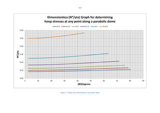
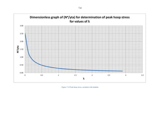
1 (2.1) General meridonal stress equation
N [∫ ( ) ]. (2.1)
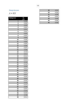
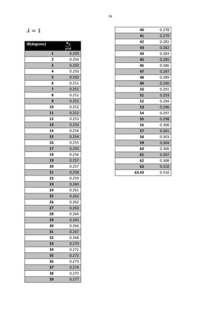
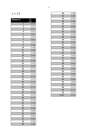
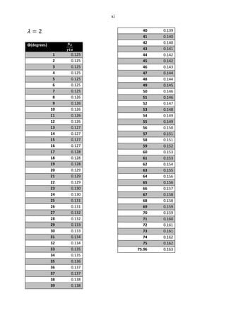
2 (2.1) General hoop stress equation
(2.1)
This equation shows that the hoop stress is a function of meridonal stress, geometric
properties as well as the loading.
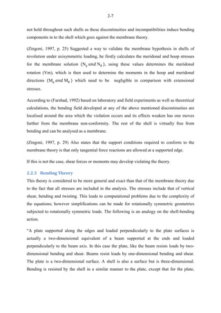
2.3.3 Deformation of Shells
The equations for the displacement of a spherical dome under axisymmetric loading were
determined by using the hoop and meridonal stresses found above. These displacements were
initially in the hoop and meridonal direction, however that for the sake of practicality, the
equations were developed such that the horizontal shell displacement as well as the rotation
of the meridian (δ and V respectively) can be calculated.
(N N ) (2.3)
* N – N (N N ) + (2.4)
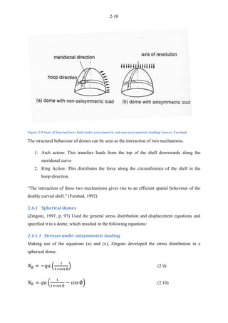
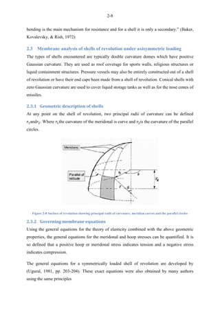
2.4 Membrane analysis of concrete domes of revolution
The membrane field of internal forces comprises of the meridonal, hoop and a membrane
shear force. However, under axisymmetric loading conditions, the membrane shear force is
zero throughout the shell and the internal force field comprises of meridonal and hoop forces
only. The directions of principal normal stresses coincide with meridonal and hoop curve and
the shear stress will be zero along these directions.

2-10
Figure 2-9 State of Internal force field under axisymmetric and non-axisymmetric loading( Source: Farshad)
The structural behaviour of domes can be seen as the interaction of two mechanisms.
1. Arch action: This transfers loads from the top of the shell downwards along the
meridonal curve
2. Ring Action: This distributes the force along the circumference of the shell in the
hoop direction.
“The interaction of these two mechanisms gives rise to an efficient spatial behaviour of the
doubly curved shell.” (Farshad, 1992)
2.4.1 Spherical domes
(Zingoni, 1997, p. 97) Used the general stress distribution and displacement equations and
specified it to a dome, which resulted in the following equations:
2.4.1.1 Stresses under axisymmetric loading
Making use of the equations (x) and (x), Zingoni developed the stress distribution in a
spherical dome.
( ) (2.9)
( ) (2.10)

2-11
From the above equations, we can see that the meridonal stress (N ) is always implies the
entire dome is under compression in the meridonal direction. However the hoop stresses are
found to be in compression in the upper region of the shell and changes to tension at a certain
point ( )
2.4.1.2 Displacements under axisymmetric loading
( ) (2.11)
(2.12)
2.4.1.3 Spherical Dome of gradually varying thickness
Zingoni analyses a spherical dome whose thickness varies along the length of its meridonal
curve. He considers that the variation of thickness only begins after a certain point along the
meridonal curve. This point can be considered to have 2-D polar co-ordinates (a,Φe )Where a
is the radius of the curve and Φe is the angle measured from the y-axis. The end point of the
curve of the curve is defined as (a, Φs).
In the section of the curve guided by co-ordinates (a, {0≤Φ≤Φe}), the weight of the shell is
considered to be uniform and the stresses due to self-weight can be calculated at any point
along this curve using Equations 2.5 & 2.6. In the remaining section of the curve guided by
polar co-ordinates (a, {Φs≤Φ≤Φe}), the thickness of the shell varies and is governed by the
equation
(2.13)
This variation in thickness causes the loading due to self-weight to vary in this section of the
shell. This requires one to return to equations 2.1 and 2.2 and derive the equations for the
stress using this varying self-weight. (Zingoni, 1997, pp. 99-103)

3-1
3 Development of closed form solutions
3.1 Assumptions
 Negative stresses imply compression and positive stresses imply tension.
 Wind loading will not be taken into account
 All bending effects will be ignored
 No shear forces are developed due to the rotational symmetry of the domes
3.2 Geometric Properties
Before explicit solutions can be formed, the geometric properties of domes of revolution will
need to be quantified.
3.2.1 Curvature
The meridonal radius of curvature can be defined by the following equation
√
(3.1)
The hoop radius of curvature is defined by
(3.2)
3.2.2 Surface area
In order to compute the surface area of a shell of revolution, the shell can be segmented into
bands of which the length of the curve can be determined. This length is then multiplied the
circumference at the point in question. (Stewart, 2006)

3-2
Figure 3-1 Computation of surface area by segmentation (Source: Stewart)
An element of the curve can be isolated, if we assume its length equals ds, then by the
following relationship seen in the image below, ds may be written it terms of dx and dy.
Figure 3-2 Arc length element
√
The length of the curve can be found using the arc length formula
∫ √ ( ) (3.3)
The arc length is then multiplied by the circumference at the point giving the surface area of
the band, which when integrated over the domain of the curve leads to the surface area of
shell.

3-3
∫ √ (3.4)
3.2.3 Loading
The loading on a shell is solely due to the self-weight of the structure.
The self-weight of any concrete structure can be defined by the unit weight of the concrete (γ)
multiplied by volume of concrete. In a shell this volume is calculated by the surface area(S)
of the shell multiplied by shell thickness (t)
(3.5)
At any point on the surface of the shell, the weight is acting vertically downwards onto the
shell. This is the resultant force of and which acts in the tangential normal directions
respectively. They can be quantified as
(3.6)
(3.7)
Figure 3-3 Loading Components due to self-weight
3.3 Method of sections for determination of stresses
In order to determine the stress distribution within a shell, the concept of equilibrium was
used to analyse the shape as described by (Zingoni, 1997) and by (Farshad, 1992). This
method is intuitive by nature as it relies simply on the balancing of forces within the shell. As

3-4
this research project only takes into account axi-symmetric loading, the only force the
structure will need to be analysed for is that of self-weight. This is purely based on membrane
theory as non axi-symmetric loading is not considered; however there are conditions to
whether the membrane theory holds under axi-symmetric loading as it is possible for
moments and shear forces to develop. These conditions were mentioned in earlier.
Consider a shell of revolution with an arbitrary meridian profile whose equation can be
defined by y= F(x) and with its axis of symmetry being the Y-axis. If a point T is identified
on this curve and a slice is taken at that point, i.e. the cap of the dome lying above point is
isolated.
Figure 3-4 Arbitrary shell profile
Based on Newton‟s Third Law, the force required by the shell below the slice to hold up the
cap is equal to force exerted by the cap on to the section below. From this we can say that
meridonal force at a point is generated due to the self-weight of the above cap. The self-
weight acts vertically while the meridonal force acts in a direction tangential to the meridian
curve at the point T.
Phi (Φ) can be defined as the angle between the positive axis of revolution and the normal to
the shell mid-surface at the point T as seen in Figure 3-4.

3-5
Figure 3-5 Force balance
The forces seen in Figure 3-5 are the self-weight of the cap (W) measured in kN and the
meridonal force .which acts along the circumference of the shell and is measured in kN/m.
If we sum the forces in the vertical direction, we obtain the following equilibrium equation:
(3.8)
Therefore N can be written explicitly as
3 (3.9) Meridonal stress equilibrium equation
(3.9)
The stress N will need to be written explicitly in terms of Φ in order to see how stresses vary
along the profile of the curve.
3.4 Parameterisation of stresses equations
The stress equations found using the methods mentioned above will be written in terms of a
parameter which will be defined as the height of the shell over the radius of the base of the
shell. These stress equations will then be plotted against the angle (Φ) for each value of the
parameter within a practical range. The results will then be discussed.

4-1
4 Parabolic Dome of Revolution
The equation of the meridian curve for the parabolic dome can be defined by the equation
(4.1)
This equation needs to satisfy the following representation of the meridian curve where
: is the distance from the axis of revolution to curve at the base of the parabola, this
will further be referred to as the radius of the parabola.
: is the distance along the axis of revolution from the base of the parabola to its apex
and will further be referred to as the height of the parabola.
: is a place holding variable which will be rewritten in terms of a, b as these are the
variables we are mainly interested in
: Defined, as the angle from the positive axis revolution to the normal of the curve.
Figure 4-1 Parameters of defined parabolic meridian
The elimination of the place holding variable k can be done by evaluating the function at the
point on the base of the parabola (a, 0). Substituting these values into equation (3.3) leads to:
(4.2)
From which k can be found to be
And ultimately the equation of the meridonal curve of the parabolic dome is

4-2
(4.3)
Due to the way the parameters of the parabola were set out, it was expected that k is negative
as this is what gives the concave shape which is required for a roofing structure to serve the
purposes for which it was intended for.
In order to have N varying with Φ, x needs to be eliminated from the equation. The critical
link between x and Φ can be found in the fact that the meridonal stress acts tangentially to the
curve at any point. And the first derivative of the meridonal curve evaluated at any point x
which gives the tangent to the curve at the point in question. The derivative can then be
equated to forming the following relationship.
(4.4)
The derivative of equation (3.4) can be found using simple differentiation techniques and lead
to the derivative being
(4.5)
Using the relationship established in equation (3.5) and equation (3.6), it is possible to obtain
an explicit equation of x in terms of Φ
(4.6)
With equation (3.7), the x-coordinate of any point along the curve can be described in terms
of the phi value. Limits for the phi values will need to be introduced as the angle cannot run
from 0 through 90 degrees because a phi value of 90 implies a vertical tangent line to the
curve, which of course does not exist. The section of the curve which will be rotated about
the y-axis has the domain . Substitution of these boundary values into equation
(3.7) yield the following limits for phi denoted as and respectively.
(4.7. a)
(4.7. b)
Substituting equation (3.7) back into (3.2) eliminates the x value and leaves us with the stress
in terms of phi.

4-3
(4.8)
The self-weight (W) is the only remaining variable which needs to be defined in terms of phi
(or x as we have the relationship between them).
The surface area of the paraboloid of revolution was found by using equation (2.5) in
conjunction with equation (3.5). The equation was then integrated making use of a place
holding variable so that the limits of integration may be in terms of x. A basic substitution
was used to evaluate the integral. The resulting surface area in terms of x was found to be:
*( ) + (4.9)
Substitution of equation (3.7) into (3.11) to eliminate x and get the surface area to be in terms
of Φ so as to be consistent with equation (3.9) to which it was eventually substituted into.
* + (4.10)
Combining equations (3.10), (3.11) and (3.12) led to the meridonal stress at any point along
the curve in terms of phi.
4 (4.11) Meridonal stress equation for parabolic dome
* + (4.11)
In order to determine the exact equation for hoop stresses ( ), the relationship developed by
(Ugural, 1981) found in equation (2.1) will be re-written with as the subject.
Equations (2.5), (2.6) and were first redefined in terms of phi using the relation in equation
(3.7). These equations along with equation (2.8) was used to eliminate and and from
the above equation.

4-4
After simplification the equation for the hoop stress was found to be
5 (4.12) Hoop stress equation for parabolic dome
* ( ) + (4.12)

5-1
5 Ellipsoidal Dome of Revolution
5.1 Method of Sections
Following the method of sections as described in chapter 3, the equation of the meridonal
curve for the ellipsoid of revolution can be defined by the equation
(5.1)
Or explicitly defined as
√
Where
: is the distance from the axis of revolution to curve at the base of the ellipsoid, this
will further be referred to as the radius of the ellipsoid.
: is the distance along the axis of revolution from the base of the parabola to its apex
and will further be referred to as the height of the ellipsoid.
: Defined, as the angle from the positive axis revolution to the normal of the curve.
Figure 5-1 Parameters of defined ellipsoidal meridian

5-2
The meridonal stress ( ) in the ellipsoidal dome under self-weight can be calculated using
equation (3.2).
(3.2)
In order to see the relationship of the meridonal stress with respect phi, will need to be
eliminated using the relationship:
(5.2)
Implicit differentiation was used to determine :
(5.3)
Substituting equation (5.3) into the relationship indicated in (5.2) allows to be explicitly
solved for in terms of phi.
(5.4)
With equation (5.4), the x-coordinate of any point along the curve can be described in terms
of the phi value; however it can be seen from equation (5.3) that at the point , there
exists a vertical tangent i.e. phi equals 90 degrees.
The loading on the ellipsoid ( ) due to the self-weight of the structure at the point above the
cut can be written in terms of the unit weight of concrete, the thickness of the dome as well as
the surface area as presented in equation (2.8)
(2.8)
Using equations (2.8) and (5.4) to eliminate and from equation (3.2)
6 (5.5) Incomplete equilibrium equation for ellipsoidal dome
( )
(5.5)
The surface area of the ellipsoid posed the greatest problem as it could not be expressed in
such a way that a relationship between phi and the surface area and subsequently the stresses
could be identified.

5-3
An alternative approach was considered.
5.2 The general stress equations for membrane theory
Making use of equations (2.1) and (2.2) the stress equations for the hoop and meridonal
stresses can be determined
N ∫ . (2.1)
(2.2)
Where
: Meridonal radius of curvature
: Hoop radius of curvature
: Radial loading component
: Tangential loading component
From equation (3.1) and (3.2), the curvatures and can be calculated, with equation (5.4)
being used to eliminate .
(5.6)
(5.7)
The loading components which were identified in chapter 3 is used in conjunction with the
curvatures found above in order to compute the stress variation within the ellipsoidal dome.
(3.6)
(3.7)
Substitution of the above equations into the general stress formula leads to:
( )
∫ (5.8)

5-4
Due to the complexity of the integral in equation (3.8), evaluation was done with the aid of an
online integral solver, Wolfram Alpha™.
Figure 5-2 Output of online integral calculator (Source: Wolfram Alpha)
The evaluated integral was then substituted back into equation (3.8). After some
simplification the equation meridonal stress was found to be:
7 (5.9) Invalid meridonal stress equation for ellipsoidal dome
( )
(5.9)
From the above equation, certain problems were identified;
 The term in the denominator
 The term in both the numerator and the denominator
 The in the numerator.
The ellipsoid was defined in such a way that phi equals zero degrees corresponds to the apex
of the ellipsoidal dome with coordinates and phi equals ninety degrees corresponds to
the base of the dome with coordinates .
If we go back and see the way was defined in terms of phi by looking at the equation
There exists a problem in the limits of phi due to the fact that at the point where , phi is
undefined, which is expected due to the vertical tangent existing there. However the lower
limit of phi can be defined as 0 corresponding to .
In equation (5.9) the constant of integration, needs to be eliminated via the substitution of
known values into the equation. The only point where the meridonal stress is known is at the
apex and its value is zero due to the fact that no load exists above the point. Substituting

5-5
And
This causes the equation to be undefined due to the term being zero in the
denominator.
The second problem is anticipated when parameterising the equation; all the terms can be
written in some ratio of height to radius except the term . Therefore it will not be possible to
observe the correlations in the stress and the ratio.
The final problem is encountered when phi equals ninety degrees; this once again leads to the
stress equation being undefined due to the term in the numerator.
Had the equation for the meridonal stress been successfully developed, the next step would
have been to determine the hoop stress by making use of equations (2.2), (3.7), (5.6) and
(5.7).
.

6-1
6 Parametric Results
6.1 Parabolic Dome of Revolution
A non-dimensional parameter for the concrete shell was defined to be lambda (λ) which was
defined as the ratio of height-to-radius of the parabolic dome.
(6.1)
Equation (6.1) was substituted in equations (4.11) and (4.12) making sure that the only
variables in the equations are lambda and phi. After simplification, the term remained in
the numerator, the resultant meridonal and hoop stresses was then divided by this term which
effectively made the left hand side of the equations dimensionless.
* + (6.2)
* ( ) + (6.3)
From the above equations we can see that for shells of the same shape (same height-to-radius
ratio λ) the stress resultant in the shell is directly proportional to radius of the dome, and
therefore also directly proportional to the height, due to the fact that lambda remains
constant. Therefore doubling the height or radius of the dome will effectively double the
hoop and meridonal stresses in the structure. The thickness of the structure also has a direct
relationship with the stress resultants this is because increasing or decreasing the thickness by
a factor will result in proportional increase or decrease to the stress resultants.
6.2 Ellipsoid of revolution
A non-dimensional parameter for the concrete shell was defined to be psi (ψ) which was
defined as the ratio of height-to-radius of the elliptical dome.
(6.4)
Psi is then substituted into equation (5.9) in order eliminate all other variables except that of
phi and psi.

6-2
(6.5)
As seen in the terms indicated in the red circles above, it is not possible to rewrite them in
terms of psi whereas all other terms in the expression can be.
Due to the reasons outlined here, it will not be possible to conduct a parametric study for the
ellipsoidal dome of revolution.

7-1
7 Discussion of Results
7.1 Parabolic dome of revolution
Non-Dimensional stress variations and plotted against the meridonal angle, Φ for
various values of λ ranging from 0.5 to 3.0 which covers most practical domes. This covers
most practical cases of the parabolic dome. From equations (4.7), it can be seen that the dome
lies within the interval which, in terms of lambda is .
Therefore the stress resultant equations are only valid within this interval. The intervals for
each corresponding value of lambda can be seen in table 1 below
Table 1 Range of phi values defining parabolic dome
λ Ranges of Φ (°)
0.5 0-45
1 0-63.4
1.5 0-71.6
2 0-76
2.5 0-78.7
3 0-80.5
7.1.1 Meridonal stress
It can be seen that the hoop stress is directly proportional to the radius of the dome as well as
the thickness of the shell, therefore doubling of either of these parameters will double the
hoop stress in the dome.
For all values of lambda, the meridonal stress remains negative (compressive) throughout the
shell. Theoretically the stress at the apex of the dome is zero; however this cannot be seen in
the graph due to the fact that the meridonal stress resultant function cannot be defined at the
point. Keeping lambda constant, it can be seen that the meridonal stress increases (in
compression) in an almost exponential trend, which is expected as the self-weight gets
cumulatively higher as you move toward the base of the dome reaching peak stress at the

7-2
base of the dome. These peaks in terms of non-dimensional stresses can be found in the
table below.
Table 2 Peak meridonal stress for corresponding values of lambda
λ Peak Stresses
0.5 -0.862
1 -0.948
1.5 -1.196
2 -1.484
2.5 -1.789
3 -2.103
From the parameterised equation (6.2) it is evident that lambda is inversely proportional to
the meridonal stress. I.e. a decrease in lambda induces an increase in the stress resultant. This
is illustrated in figure 7.1 below where for example at a constant phi value of 45°; the
meridonal stresses for lambda equalling 3; 2.5; 2; 1.5; 1 and 0.5 the non-dimensional
meridonal stress is found to be -0.144; -0.172; -0.215; -0.287; -0.431 and -0.862 respectively.
However, due to the fact that a higher value of lambda increases the phi interval, the higher
meridonal stresses will be found at the base of slender parabolic domes ( ) as seen
when comparing the peak non-dimensionless meridonal stresses. Consider the case of lambda
equal to 0.5; the peak non-dimensional stress occurs at 45° and equals -0.862. Looking at
lambda equal to 3; the peak non-dimensional stress occurs at 80.5° and equals -2.103.
A graph showing how the peak non-dimensional stress varies with lambda was developed
seen in Figure 7.2. There exists a value of lambda where the peak stress at the base of the
dome is at a minimum and any increase or decrease in lambda will cause the peak stress to
increase. This minimum occurs at a lambda value of 0.6 and has a corresponding non-
dimensional stress value of -0.847.

7-3
Figure 7-1 Meridonal stress distribution in parabolic dome
-2.50
-2.00
-1.50
-1.00
-0.50
0.00
0 10 20 30 40 50 60 70 80 90
Nᶲ/γta
Φ(degrees)
Dimensionless (Nᶲ/γta) Graph for determining
meridonal stresses at any point along a parabolic dome
λ=3 λ=2.5 λ=2 λ=1.5 λ=1 λ=0.5

7-4
Figure 7-2 Peak meridonal stress variation with lambda
-3.00
-2.50
-2.00
-1.50
-1.00
-0.50
0.00
0 0.5 1 1.5 2 2.5 3 3.5
Nᶲ/γta
λ
Dimensionless graph of (Nᶲ/γta) for determination of peak meridonal
stress for values of λ

7-5
7.1.2 Hoop stress
It can be seen that the hoop stress is directly proportional to the radius of the dome aswell as
the thickness of the shell, therefore doubling of either of these parameters will double the
hoop stress in the dome.
For all values of lambda, the hoop stress remains positive (tensile) throughout the shell. .
Theoretically the stress at the apex of the dome is zero; however this cannot be seen in the
graph due to the fact that the hoop stress resultant function cannot be defined at the point.
For a constant value of lambda, the hoop stress follows an almost linear trend along the
profile of the curve. For higher values of lambda, there is a shallow gradient and the change
in stress resultant from the apex to the base is minimal, whereas for smaller values of lambda,
there is a steeper gradient and there is a considerable difference in stresses at the apex and
base.
For example for a lambda value of 0.5, the non-dimensional apex and base stresses are 0.5
and 0.57 respectively. Compare those values to a lambda value of 3, with non-dimensional
apex and base stresses 0.09 and 0.11 respectively. A possible explanation for this is that as
the dome becomes more slender, more of the stress gets transferred through meridonal action
rather than hoop action. The peak hoop stresses at the base of the dome for each value of
lambda can be found in the table below.
Table 3 Peak hoop stress for corresponding values of lambda
λ Peak Stresses
0.5 0.569
1 0.310
1.5 0.214
2 0.163
2.5 0.131
3 0.110
As with meridonal stress, the hoop stress within the dome is also inversely proportional to
lambda. As lambda decreases, the hoop stresses throughout the entire range of shell increases.
This trend can be seen in figure 7.3 below. At any point along the shell profile for lambda
equal to 0.5, the non-dimensional hoop stress is considerably larger than at any corresponding
point along the profile of lambda equal to 3. The peak stress for values of lambda ranging

7-6
from 0 to 3 was graphed; the peak stresses follow a hyperbolic trend where they are
maximum at low values of lambda and minimum at high values.
Due to the weakness of concrete in tension reinforcement might be required. If one assumes
that a minimum tensile stress of 2 MPa will cause failure with in the dome, it is possible to
identify under which geometric conditions this will occur and where reinforcement will be
required. From the trends seen in the non-dimensional charts, for lambda values of 1.5 and
greater, tensile reinforcement will only be required for very large structures due to the low
values of hoop stresses.
For example, consider a lambda value of 0.5 for a structure with height and base of 81m and
162m respectively. It is possible to calculate from which point tensile reinforcement will be
required. The point at which the tensile stress exceeds 2 MPa occurs at a phi value of 20° and
continues through to a phi value 45°. The corresponding x values can be calculated by using
equation (4.6).

7-7
Figure 7-3 Hoop stress distribution in parabolic dome
0.00
0.10
0.20
0.30
0.40
0.50
0.60
0 10 20 30 40 50 60 70 80 90
Nᶱ/γta
(Φ)Degrees
Dimensionless (Nᶱ/γta) Graph for determining
hoop stresses at any point along a parabolic dome
λ=3 λ=2.5 λ=2 λ=1.5 λ=1 λ=0.5

7-8
Figure 7-4 Peak hoop stress variation with lambda
0.00
0.50
1.00
1.50
2.00
2.50
3.00
0 0.5 1 1.5 2 2.5 3 3.5
Nᶱ/γta
λ
Dimensionless graph of (Nᶱ/γta) for determination of peak hoop stress
for values of λ

8-1
8 Numerical Example
Design a 100m high, 50m wide parabolic dome with an assumed thickness of 0.5m
 Calculate λ equation (6.1)
 Plot non-dimensional meridonal and hoop stress charts for λ equals 2 (Appendix A)
 Multiply non-dimensional values by to obtain stress resultants
The peak meridonal stress will be calculated by
The peak hoop stress will be calculated by
No tensile reinforcement will be required.

9-1
9 Conclusion and Recommendations
The hoop and meridonal stress of the parabolic dome has been expressed in terms of a
geometric parameter λ which enabled the study of stress distributions with in the dome. Many
challenges were encountered with the ellipsoidal dome and ultimately it was not possible to
express the equations in terms of a single governing geometric property.
Focussing on the parabolic investigation, it was found that both the hoop and meridonal
stresses are directly proportional to both the thickness and base radius of the structure and
any change in these variables will produce a proportional change in the stress resultants.
The meridonal stress within the dome was found to increase as lambda decreased, however,
greater values of lambda implied a greater structure which in turn leads to a greater range of
phi values. This allows the peak meridonal stresses for higher values of lambda to surpass
that of lower values of lambda.
The hoop stress with in the dome followed the same inversely proportional relationship as
that of meridonal stress. However in the case of the hoop stress, a lower value of lambda
shows that the hoop stress throughout the structure is greater than the hoop stress at any point
along the profile of a dome with a higher value of lambda.
The design charts were developed for the hoop and meridonal stress distribution within a
parabolic dome for lambda values ranging from 0.5 to 3. These charts can be used to obtain
the stresses at any point along the profile of the parabolic.
This study can be further developed by increasing the scope of the investigation to include
the effects of wind loading on the structure. Doing so will induce shear and bending forces in
the structure.
Further development of the uncompleted ellipsoidal stress equations will need to be further
developed in order to complete a parametric study on this shaped dome.

10-1
10 References
Baker, E. H., Kovalevsky, L., & Rish, F. L. (1972). Structural Analysis of Shells.
Farshad, M. (1992). Design and Analysis of Shell Structures.
Stewart, J. (2006). Calculus Concepts & Contexts 3.
Ugural, A. (1981). Stresses in Plates & Shells.
Zingoni, A. (1997). Shell Structures In Civil & Mechanical Engineering.
KRIVOSHAPKO, S.N., (2007). Research on General and Axisymmetric Ellipsoidal Shells
Used as Domes, Pressure Vessels, and Tanks. Applied Mechanics Reviews, 60(6), pp. 336.
NEMENYI, P. and TRUESDELL, C., (1943). A Stress Function for the Membrane Theory of
Shells of Revolution. Proceedings of the National Academy of Sciences of the United States of
America, 29(5), pp. pp. 159-162.
WAN, F.Y.M. and WEINITSCHKE, H.J., (1988). On shells of revolution with the Love-
Kirchhoff hypotheses. Journal of Engineering Mathematics, 22(4), pp. 285-334.
ZINGONI, A., (2002). Parametric stress distribution in shell-of-revolution sludge digesters
of parabolic ogival form. Thin-Walled Structures, 40(7–8), pp. 691-702.

ii
Appendix A: Design tables for
parabolic dome
Meridonal stresses
Φ(degrees)
1 -0.500
2 -0.500
3 -0.501
4 -0.502
5 -0.503
6 -0.504
7 -0.506
8 -0.507
9 -0.509
10 -0.512
11 -0.514
12 -0.517
13 -0.520
14 -0.523
15 -0.527
16 -0.531
17 -0.535
18 -0.539
19 -0.544
20 -0.549
21 -0.555
22 -0.561
23 -0.567
24 -0.574
25 -0.581
26 -0.588
27 -0.596
28 -0.605
29 -0.614
30 -0.623
31 -0.633
32 -0.644
33 -0.655
34 -0.667
35 -0.680
36 -0.694
37 -0.708
38 -0.723
39 -0.739
40 -0.757
41 -0.775
42 -0.795
43 -0.816
44 -0.838
45 -0.862

iii
Φ(degrees)
1 -0.250
2 -0.250
3 -0.251
4 -0.251
5 -0.251
6 -0.252
7 -0.253
8 -0.254
9 -0.255
10 -0.256
11 -0.257
12 -0.258
13 -0.260
14 -0.262
15 -0.263
16 -0.265
17 -0.267
18 -0.270
19 -0.272
20 -0.275
21 -0.277
22 -0.280
23 -0.283
24 -0.287
25 -0.290
26 -0.294
27 -0.298
28 -0.302
29 -0.307
30 -0.312
31 -0.317
32 -0.322
33 -0.328
34 -0.334
35 -0.340
36 -0.347
37 -0.354
38 -0.362
39 -0.370
40 -0.378
41 -0.388
42 -0.397
43 -0.408
44 -0.419
45 -0.431
46 -0.444
47 -0.457
48 -0.472
49 -0.488
50 -0.505
51 -0.523
52 -0.543
53 -0.564
54 -0.587
55 -0.613
56 -0.640
57 -0.670
58 -0.702
59 -0.738
60 -0.778
61 -0.821
62 -0.870
63 -0.923
63.43 -0.948

iv
Φ(degrees)
1 -0.167
2 -0.167
3 -0.167
4 -0.167
5 -0.168
6 -0.168
7 -0.169
8 -0.169
9 -0.170
10 -0.171
11 -0.171
12 -0.172
13 -0.173
14 -0.174
15 -0.176
16 -0.177
17 -0.178
18 -0.180
19 -0.181
20 -0.183
21 -0.185
22 -0.187
23 -0.189
24 -0.191
25 -0.194
26 -0.196
27 -0.199
28 -0.202
29 -0.205
30 -0.208
31 -0.211
32 -0.215
33 -0.218
34 -0.222
35 -0.227
36 -0.231
37 -0.236
38 -0.241
39 -0.246
40 -0.252
41 -0.258
42 -0.265
43 -0.272
44 -0.279
45 -0.287
46 -0.296
47 -0.305
48 -0.315
49 -0.325
50 -0.337
51 -0.349
52 -0.362
53 -0.376
54 -0.392
55 -0.408
56 -0.427
57 -0.447
58 -0.468
59 -0.492
60 -0.519
61 -0.548
62 -0.580
63 -0.616
64 -0.655
65 -0.700
66 -0.751
67 -0.808
68 -0.873
69 -0.947
70 -1.033
71 -1.132
71.57 -1.196

v
Φ(degrees)
1 -0.125
2 -0.125
3 -0.125
4 -0.125
5 -0.126
6 -0.126
7 -0.126
8 -0.127
9 -0.127
10 -0.128
11 -0.129
12 -0.129
13 -0.130
14 -0.131
15 -0.132
16 -0.133
17 -0.134
18 -0.135
19 -0.136
20 -0.137
21 -0.139
22 -0.140
23 -0.142
24 -0.143
25 -0.145
26 -0.147
27 -0.149
28 -0.151
29 -0.153
30 -0.156
31 -0.158
32 -0.161
33 -0.164
34 -0.167
35 -0.170
36 -0.173
37 -0.177
38 -0.181
39 -0.185
40 -0.189
41 -0.194
42 -0.199
43 -0.204
44 -0.210
45 -0.215
46 -0.222
47 -0.229
48 -0.236
49 -0.244
50 -0.252
51 -0.262
52 -0.271
53 -0.282
54 -0.294
55 -0.306
56 -0.320
57 -0.335
58 -0.351
59 -0.369
60 -0.389
61 -0.411
62 -0.435
63 -0.462
64 -0.492
65 -0.525
66 -0.563
67 -0.606
68 -0.654
69 -0.710
70 -0.774
71 -0.849
72 -0.936
73 -1.039
74 -1.162
75 -1.310
75.96 -1.484

vi
.5
Φ(degrees)
1 -0.100
2 -0.100
3 -0.100
4 -0.100
5 -0.101
6 -0.101
7 -0.101
8 -0.101
9 -0.102
10 -0.102
11 -0.103
12 -0.103
13 -0.104
14 -0.105
15 -0.105
16 -0.106
17 -0.107
18 -0.108
19 -0.109
20 -0.110
21 -0.111
22 -0.112
23 -0.113
24 -0.115
25 -0.116
26 -0.118
27 -0.119
28 -0.121
29 -0.123
30 -0.125
31 -0.127
32 -0.129
33 -0.131
34 -0.133
35 -0.136
36 -0.139
37 -0.142
38 -0.145
39 -0.148
40 -0.151
41 -0.155
42 -0.159
43 -0.163
44 -0.168
45 -0.172
46 -0.177
47 -0.183
48 -0.189
49 -0.195
50 -0.202
51 -0.209
52 -0.217
53 -0.226
54 -0.235
55 -0.245
56 -0.256
57 -0.268
58 -0.281
59 -0.295
60 -0.311
61 -0.329
62 -0.348
63 -0.369
64 -0.393
65 -0.420
66 -0.450
67 -0.485
68 -0.524
69 -0.568
70 -0.620
71 -0.679
72 -0.749
73 -0.831
74 -0.930
75 -1.048
76 -1.193
77 -1.372
78 -1.597
78.69 -1.789

vii
Φ(degrees)
1 -0.083
2 -0.083
3 -0.084
4 -0.084
5 -0.084
6 -0.084
7 -0.084
8 -0.085
9 -0.085
10 -0.085
11 -0.086
12 -0.086
13 -0.087
14 -0.087
15 -0.088
16 -0.088
17 -0.089
18 -0.090
19 -0.091
20 -0.092
21 -0.092
22 -0.093
23 -0.094
24 -0.096
25 -0.097
26 -0.098
27 -0.099
28 -0.101
29 -0.102
30 -0.104
31 -0.106
32 -0.107
33 -0.109
34 -0.111
35 -0.113
36 -0.116
37 -0.118
38 -0.121
39 -0.123
40 -0.126
41 -0.129
42 -0.132
43 -0.136
44 -0.140
45 -0.144
46 -0.148
47 -0.152
48 -0.157
49 -0.163
50 -0.168
51 -0.174
52 -0.181
53 -0.188
54 -0.196
55 -0.204
56 -0.213
57 -0.223
58 -0.234
59 -0.246
60 -0.259
61 -0.274
62 -0.290
63 -0.308
64 -0.328
65 -0.350
66 -0.375
67 -0.404
68 -0.436
69 -0.473
70 -0.516
71 -0.566
72 -0.624
73 -0.693
74 -0.775
75 -0.873
76 -0.994
77 -1.143
78 -1.331
79 -1.573
80 -1.890
80.54 -2.103

viii
Hoop stresses
Φ(degrees)
1 0.500
2 0.500
3 0.500
4 0.501
5 0.501
6 0.501
7 0.502
8 0.502
9 0.503
10 0.504
11 0.505
12 0.505
13 0.506
14 0.507
15 0.508
16 0.510
17 0.511
18 0.512
19 0.513
20 0.515
21 0.516
22 0.518
23 0.520
24 0.521
25 0.523
26 0.525
27 0.527
28 0.529
29 0.531
30 0.533
31 0.535
32 0.537
33 0.539
34 0.541
35 0.544
36 0.546
37 0.548
38 0.551
39 0.553
40 0.556
41 0.558
42 0.561
43 0.564
44 0.566
45 0.569

ix
Φ(degrees)
1 0.250
2 0.250
3 0.250
4 0.250
5 0.250
6 0.251
7 0.251
8 0.251
9 0.252
10 0.252
11 0.252
12 0.253
13 0.253
14 0.254
15 0.254
16 0.255
17 0.255
18 0.256
19 0.257
20 0.257
21 0.258
22 0.259
23 0.260
24 0.261
25 0.262
26 0.262
27 0.263
28 0.264
29 0.265
30 0.266
31 0.267
32 0.268
33 0.270
34 0.271
35 0.272
36 0.273
37 0.274
38 0.275
39 0.277
40 0.278
41 0.279
42 0.281
43 0.282
44 0.283
45 0.285
46 0.286
47 0.287
48 0.289
49 0.290
50 0.291
51 0.293
52 0.294
53 0.296
54 0.297
55 0.298
56 0.300
57 0.301
58 0.303
59 0.304
60 0.306
61 0.307
62 0.308
63 0.310
63.43 0.310

x
Φ(degrees)
1 0.167
2 0.167
3 0.167
4 0.167
5 0.167
6 0.167
7 0.167
8 0.167
9 0.168
10 0.168
11 0.168
12 0.168
13 0.169
14 0.169
15 0.169
16 0.170
17 0.170
18 0.171
19 0.171
20 0.172
21 0.172
22 0.173
23 0.173
24 0.174
25 0.174
26 0.175
27 0.176
28 0.176
29 0.177
30 0.178
31 0.178
32 0.179
33 0.180
34 0.180
35 0.181
36 0.182
37 0.183
38 0.184
39 0.184
40 0.185
41 0.186
42 0.187
43 0.188
44 0.189
45 0.190
46 0.191
47 0.191
48 0.192
49 0.193
50 0.194
51 0.195
52 0.196
53 0.197
54 0.198
55 0.199
56 0.200
57 0.201
58 0.202
59 0.203
60 0.204
61 0.205
62 0.206
63 0.206
64 0.207
65 0.208
66 0.209
67 0.210
68 0.211
69 0.212
70 0.213
71.57 0.214

xi
Φ(degrees)
1 0.125
2 0.125
3 0.125
4 0.125
5 0.125
6 0.125
7 0.125
8 0.126
9 0.126
10 0.126
11 0.126
12 0.126
13 0.127
14 0.127
15 0.127
16 0.127
17 0.128
18 0.128
19 0.128
20 0.129
21 0.129
22 0.129
23 0.130
24 0.130
25 0.131
26 0.131
27 0.132
28 0.132
29 0.133
30 0.133
31 0.134
32 0.134
33 0.135
34 0.135
35 0.136
36 0.137
37 0.137
38 0.138
39 0.138
40 0.139
41 0.140
42 0.140
43 0.141
44 0.142
45 0.142
46 0.143
47 0.144
48 0.144
49 0.145
50 0.146
51 0.146
52 0.147
53 0.148
54 0.149
55 0.149
56 0.150
57 0.151
58 0.151
59 0.152
60 0.153
61 0.153
62 0.154
63 0.155
64 0.156
65 0.156
66 0.157
67 0.158
68 0.158
69 0.159
70 0.159
71 0.160
72 0.161
73 0.161
74 0.162
75 0.162
75.96 0.163

xii
Φ(degrees)
1 0.100
2 0.100
3 0.100
4 0.100
5 0.100
6 0.100
7 0.100
8 0.100
9 0.101
10 0.101
11 0.101
12 0.101
13 0.101
14 0.101
15 0.102
16 0.102
17 0.102
18 0.102
19 0.103
20 0.103
21 0.103
22 0.104
23 0.104
24 0.104
25 0.105
26 0.105
27 0.105
28 0.106
29 0.106
30 0.107
31 0.107
32 0.107
33 0.108
34 0.108
35 0.109
36 0.109
37 0.110
38 0.110
39 0.111
40 0.111
41 0.112
42 0.112
43 0.113
44 0.113
45 0.114
46 0.114
47 0.115
48 0.115
49 0.116
50 0.117
51 0.117
52 0.118
53 0.118
54 0.119
55 0.119
56 0.120
57 0.121
58 0.121
59 0.122
60 0.122
61 0.123
62 0.123
63 0.124
64 0.124
65 0.125
66 0.125
67 0.126
68 0.127
69 0.127
70 0.128
71 0.128
72 0.128
73 0.129
74 0.129
75 0.130
76 0.130
77 0.131
78 0.131
78.69 0.131

xiii
Φ(degrees)
1 0.083
2 0.083
3 0.083
4 0.083
5 0.083
6 0.084
7 0.084
8 0.084
9 0.084
10 0.084
11 0.084
12 0.084
13 0.084
14 0.085
15 0.085
16 0.085
17 0.085
18 0.085
19 0.086
20 0.086
21 0.086
22 0.086
23 0.087
24 0.087
25 0.087
26 0.087
27 0.088
28 0.088
29 0.088
30 0.089
31 0.089
32 0.089
33 0.090
34 0.090
35 0.091
36 0.091
37 0.091
38 0.092
39 0.092
40 0.093
41 0.093
42 0.094
43 0.094
44 0.094
45 0.095
46 0.095
47 0.096
48 0.096
49 0.097
50 0.097
51 0.098
52 0.098
53 0.099
54 0.099
55 0.099
56 0.100
57 0.100
58 0.101
59 0.101
60 0.102
61 0.102
62 0.103
63 0.103
64 0.104
65 0.104
66 0.105
67 0.105
68 0.105
69 0.106
70 0.106
71 0.107
72 0.107
73 0.107
74 0.108
75 0.108
76 0.108
77 0.109
78 0.109
79 0.109
80 0.110
80.54 0.110

xiv
Appendix B: Logbook
Date Comments
20/09 Collected Journals
Met with Prof Zingoni to arrange a meeting for 21/09
21/09 Met with Prof Zingoni
Told me to redefine stress equations in terms of spherical
coordinates
22-24/09 Long weekend
25/09 Obtained Template for thesis document
Obtained masters thesis for referencing purposes
Made contact with Deon Solomons in the maths department
26/09 Continued work on deriving equations
Setup meeting with Dr Neil Roberston for 27/09 at 10:00am
27/09 Met with Dr Robertson
Told me to try cylindrical co-ordinates as the shapes are symmetrical
28/09 Formatted Thesis Document
Placed headings and sub-headings
Inserted comments
29-30/09 Weekend
1/10/2012 Continued work on derivation of equations
Emailed Prof Zingoni
2/10/2012 Continued work on derivation of equations
No reply from Prof Zingoni
3/10/2012 Continued work on derivations
Re-emailed Prof Zingoni

xv
In the space of 3 days, Naweed Kahaar received 2 responses from
Prof Zingoni
4/10/2012 Created excel log book
5/10/2012 Arrangend meeting with Zingoni
6-7/10/2012 Weekend
8/10/2012 Meeting with Zingoni
8-14/10/2012 Continued work on derivations
15-21/10/2012 Prepared draft for submission
22/10/2012 Submitted draft
29/10/2012 Received feed back from draft
30/10-7/11 Attempted derivations of ellipsoidal shell
7-10/11/2012 Final editing
11/11/2012 Print and bound
12/11/2012 Submission

Thesis 2012

Recommended

Recommended

More Related Content

Viewers also liked

Viewers also liked (13)

Similar to Thesis 2012

Similar to Thesis 2012 (20)

Thesis 2012