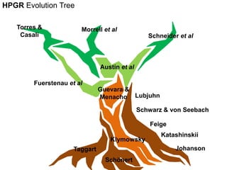
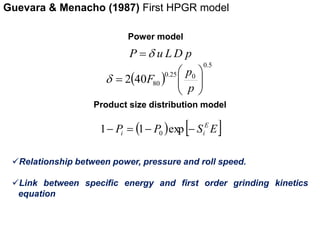
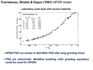
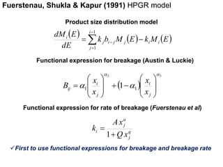
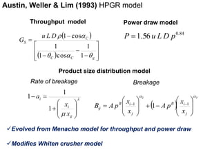
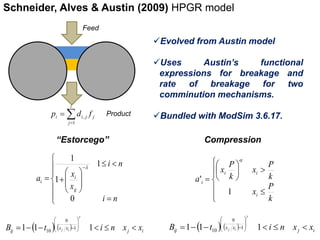
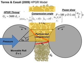
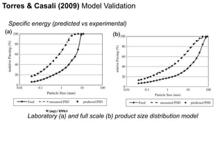
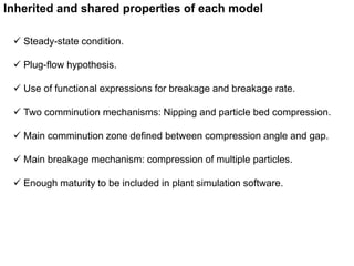
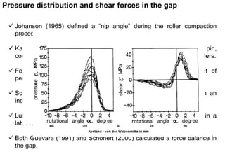
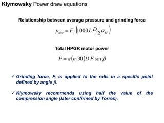
1. The document traces the evolution of models for high-pressure grinding rolls (HPGR) from early conceptual models in the 1980s to recent sophisticated models. 2. Early models focused on relating power draw, pressure, and roll speed, while later models incorporated functional expressions for breakage rates and product size distributions. 3. Breakthrough studies in the 1960s-1990s improved understanding of pressure distributions and forces in the HPGR gap, leading to more accurate power draw models. 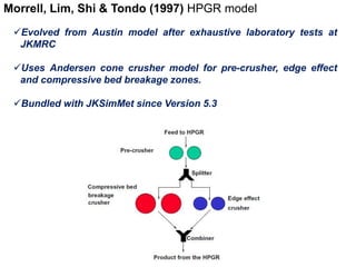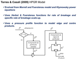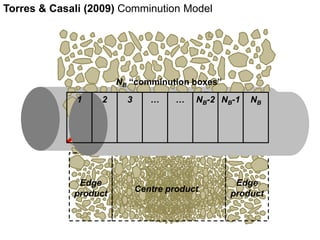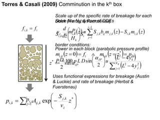4. Recent models build on prior work, using advanced functions for breakage rates and accounting for edge and center product zones with pressure profiles.

1. The evolution of HPGR
Modelling
Roberto Carlos Medrano Nina

3. From Napier-Munn et al., 1996.
HPGR Schema

4. TAGGART (1954) Spring Roll Crusher
aC
d100/2
xg/2
D/2
D/2
First equation to describe a compression angle
D x
cos a  8 a
10
   


100
C
g
C D d

5. EARLY MODELS
The Guevara & Menacho model (1987)
The Fuerstenau, Shukla & Kapur model (1991)
The Austin, Weller & Lim model (1993)

6. Guevara & Menacho (1987) First HPGR model
Power model
P  u LD p

p
0.25 0
 
0.5

80 2 40 



 
F
p
Product size distribution model
P  P   S E E
i i 1  1 exp  0
Relationship between power, pressure and roll speed.
Link between specific energy and first order grinding kinetics
equation

7. Fuerstenau, Shukla & Kapur (1991) HPGR model
Laboratory scale tests with several materials
HPGR PSD are similar to Ball Mills PSD after long grinding times
PSD are self-similar: Modified tumbling mills grinding equations
could be used for HPGRs

8. Fuerstenau, Shukla & Kapur (1991) HPGR model
Product size distribution model
 
k b M E k M E
dM E
i  
dE
i i
i
j
j i j j



1
1
Functional expression for breakage (Austin & Luckie)
a a
2 3

 


x
i
a a
1 1 1






ij x

 







i
j
j
x
x
B
Functional expression for rate of breakage (Fuerstenau et al)
q
j
a
j
Ax
i Q x
k


1
First to use functional expressions for breakage and breakage rate

9. Austin, Weller & Lim (1993) HPGR model
Throughput model
 

 a
C
1
1 cos
   


 






C C g
S
u LD
G
 a 1

1
1 cos
Power draw model
0.84 P 1.56 u LD p
Product size distribution model
Rate of breakage



x
 






 
g
i
i
x
a
1
1
1
a a
2 3






x
x
  
A p
Evolved from Menacho model for throughput and power draw
Modifies Whiten crusher model
 
1 1 1






 




j
B i
j
B i
ij x
x
B A p
Breakage

10. BREAKTHROUGH STUDIES
Peripheral and axial pressure distribution
Power draw models

11. Pressure distribution and shear forces in the gap
 Johanson (1965) defined a “nip angle” during the roller compaction
process.
 Katashinski (1966) was the first to measure, with a sensor pin,
compressive and shear forces during the compression of metal powders.
 Feige (1989) used the sensor-pin method for the measurement of
peripheral and axial pressure distributions in a roller crusher.
 Schwarz and von Seebach (1990) discovered the “edge effect” in an
industrial HPGR.
 Lubjuhn (1992) characterized the peripheral pressure distribution in a
lab-scale HPGR using quartz and limestone.
 Both Guevara (1991) and Schönert (2000) calculated a force balance in
the gap.

12. Klymowsky Power draw equations
Relationship between average pressure and grinding force
ave  IP 
p F LD a
2
 1000
Total HPGR motor power
P  n 30DF sin
 Grinding force, F, is applied to the rolls in a specific point
defined by angle  .
 Klymowsky recommends using half the value of the
compression angle (later confirmed by Torres).

13. RECENT MODELS
The Morrell, Lim, Shi & Tondo Model (1997)
The Schneider, Alves & Austin Model (2009)
The Torres & Casali Model (2009)

14. Morrell, Lim, Shi & Tondo (1997) HPGR model
Evolved from Austin model after exhaustive laboratory tests at
JKMRC
Uses Andersen cone crusher model for pre-crusher, edge effect
and compressive bed breakage zones.
Bundled with JKSimMet since Version 5.3

15. Schneider, Alves & Austin (2009) HPGR model
i i j j p d f







Product Bundled with ModSim 3.6.17.
“Estorcego”
i n
 









 

i n
x
x
a
i
g
i
0
1
1
1



ij B t i n x x j i        
    j i
1 1 x x
1 1

 

9
10

Evolved from Austin model
Uses Austin’s functional
expressions for breakage and
rate of breakage for two
comminution mechanisms.
Compression


 




 




P
P
k
i i
x
k
x
P
k
x
a
i
i
1
'
a


ij B t i n x x j i        
    j i
1 1 x x
1 1

 

9
10

Feed


i
j
1
,

16. Torres & Casali (2009) HPGR Model
Evolved from Morrell and Fuerstenau model and Klymowsky power
equations
Uses Herbst & Fuerstenau functions for rate of breakage and
specific rate of breakage scale-up.
Uses a pressure profile function to model edge and centre
products.

17.    
1
cos 2
    
xc
HPGR Throughput
G x Lu S C g  3600 
aIP Pressure

xg
u
C



u
Moveable Roll
D x L
Single particle
Compression
x > xC
Particle bed
compression






g C
f
IP g g
x D
x D x D
D 
a
4
2


Compression angle P p D L IP u 


2
100 sin
a
Power draw
Torres & Casali (2009) HPGR Model

18. Torres & Casali (2009) Comminution Model
Parabolic pressure profile
Centre product
Edge
product
Edge
product
NB “comminution boxes”
1 2 3 N NB-1 NB B… … -2

19. Torres & Casali (2009) Comminution in the kth box
Scale up of the specific rate of breakage for each
block (Herbst & Fuerstenau)
Solve N x NB system of ODEs
P

, , ,  

 ,
v k
i k i k
S 
i k S
z i k j k ij j k , ,


d
j k
S
i k i f f  ,
   

 
 
z
i k ij k 
i
j
z
v
p A
1
, *
, , exp
IP
D
z sina
2
* 
i k p ,
m z S b m z S m z
dz
i
j
1
1


border conditions:
m  z  f m  z z *
 p i k i i k i ,
k  0     , ,  L 2 y
2

IP k
  
 








NB
j j
k
L y
P p LD u
1
2 2
4
4
2
100 sin
a
E
i
k
H

 

Power in each block (parabolic pressure profile)
Uses functional expressions for breakage (Austin
& Luckie) and rate of breakage (Herbst &
Fuerstenau)

20. Torres & Casali (2009) Model Validation
Specific energy (predicted vs experimental)
Damp sample
Laboratory (a) and full scale (b) product size distribution model

21. Inherited and shared properties of each model
 Steady-state condition.
 Plug-flow hypothesis.
 Use of functional expressions for breakage and breakage rate.
 Two comminution mechanisms: Nipping and particle bed compression.
 Main comminution zone defined between compression angle and gap.
 Main breakage mechanism: compression of multiple particles.
 Enough maturity to be included in plant simulation software.

22. Schönert
Taggart
Austin et al
Schneider et al
Torres & Morrell et al
Casali
Fuerstenau et al
Lubjuhn
Schwarz & von Seebach
Klymowsky
Katashinskii
Johanson
Feige
Guevara &
Menacho
HPGR Evolution Tree