Download free for 30 days
Sign in
Upload
Language (EN)
Support
Business
Mobile
Social Media
Marketing
Technology
Art & Photos
Career
Design
Education
Presentations & Public Speaking
Government & Nonprofit
Healthcare
Internet
Law
Leadership & Management
Automotive
Engineering
Software
Recruiting & HR
Retail
Sales
Services
Science
Small Business & Entrepreneurship
Food
Environment
Economy & Finance
Data & Analytics
Investor Relations
Sports
Spiritual
News & Politics
Travel
Self Improvement
Real Estate
Entertainment & Humor
Health & Medicine
Devices & Hardware
Lifestyle
Change Language
Language
English
Español
Português
Français
Deutsche
Cancel
Save
EN
YN
Uploaded by
Yukihiro NAKAJIMA
PDF, PPTX
1,760 views
空間統計を使って地価分布図を描いてみる
Tokyo.R #64で発表したスライドになります。 間違いの指摘やこうすればもっとよいなどありましたら、ご連絡ください。
Data & Analytics
◦
Read more
3
Save
Share
Embed
Embed presentation
Download
Download as PDF, PPTX
1
/ 36
2
/ 36
3
/ 36
4
/ 36
5
/ 36
6
/ 36
7
/ 36
8
/ 36
9
/ 36
10
/ 36
11
/ 36
12
/ 36
13
/ 36
14
/ 36
15
/ 36
16
/ 36
17
/ 36
18
/ 36
19
/ 36
20
/ 36
21
/ 36
22
/ 36
23
/ 36
24
/ 36
25
/ 36
26
/ 36
27
/ 36
28
/ 36
29
/ 36
30
/ 36
31
/ 36
32
/ 36
33
/ 36
34
/ 36
35
/ 36
36
/ 36
More Related Content
PDF
データを読む感性
by
Hideo Hirose
PPTX
M1gp -Who’s (Not) Talking to Whom?-
by
Takashi Kawamoto
PDF
20140625 google earthの最前線
by
Taichi Furuhashi
PPTX
Effective Java 輪読会 項目69-70追加
by
Appresso Engineering Team
PDF
データを読み取る感性
by
Hideo Hirose
PDF
RでGISハンズオンセッション
by
arctic_tern265
DOCX
Rデモ03_データ分析編2016
by
wada, kazumi
PDF
Rを用いたGIS
by
Mizutani Takayuki
データを読む感性
by
Hideo Hirose
M1gp -Who’s (Not) Talking to Whom?-
by
Takashi Kawamoto
20140625 google earthの最前線
by
Taichi Furuhashi
Effective Java 輪読会 項目69-70追加
by
Appresso Engineering Team
データを読み取る感性
by
Hideo Hirose
RでGISハンズオンセッション
by
arctic_tern265
Rデモ03_データ分析編2016
by
wada, kazumi
Rを用いたGIS
by
Mizutani Takayuki
Similar to 空間統計を使って地価分布図を描いてみる
PDF
R入門とgoogle map +α
by
kobexr
PDF
状態空間モデルの実行方法と実行環境の比較
by
Hiroki Itô
PPTX
Feature Selection with R / in JP
by
Sercan Ahi
PPTX
StanとRでベイズ統計モデリングに関する読書会(Osaka.stan) 第四章
by
nocchi_airport
PPTX
行動圏推定の基礎知識2014.8
by
Hiroaki Ishii
PDF
マルコフ連鎖モンテカルロ法入門-2
by
Nagi Teramo
PDF
ggplot2をつかってみよう
by
Hiroki Itô
PPTX
forestFloorパッケージを使ったrandomForestの感度分析
by
Satoshi Kato
PPTX
R seminar on igraph
by
Kazuhiro Takemoto
PDF
機械学習コン講評
by
Hiromu Yakura
PDF
Yamadai.Rデモンストレーションセッション
by
考司 小杉
PDF
ハイブリッド型樹木法
by
Mitsuo Shimohata
PDF
Fisher Vectorによる画像認識
by
Takao Yamanaka
PDF
GRASSセミナー応用編
by
Kanetaka Heshiki
PDF
Foss4 gマイクロジオデータ解析入門
by
Hiroaki Sengoku
PDF
モンテカルロサンプリング
by
Kosei ABE
PDF
カテゴリカルデータの解析 (Kashiwa.R#3)
by
Takumi Tsutaya
PDF
ビジネス基礎講座:統計学入門 introduction to statistics
by
Masaaki Nabeshima
PDF
Rでシステムバイオロジー
by
弘毅 露崎
PPTX
Car rmodel
by
Akichika Miyamoto
R入門とgoogle map +α
by
kobexr
状態空間モデルの実行方法と実行環境の比較
by
Hiroki Itô
Feature Selection with R / in JP
by
Sercan Ahi
StanとRでベイズ統計モデリングに関する読書会(Osaka.stan) 第四章
by
nocchi_airport
行動圏推定の基礎知識2014.8
by
Hiroaki Ishii
マルコフ連鎖モンテカルロ法入門-2
by
Nagi Teramo
ggplot2をつかってみよう
by
Hiroki Itô
forestFloorパッケージを使ったrandomForestの感度分析
by
Satoshi Kato
R seminar on igraph
by
Kazuhiro Takemoto
機械学習コン講評
by
Hiromu Yakura
Yamadai.Rデモンストレーションセッション
by
考司 小杉
ハイブリッド型樹木法
by
Mitsuo Shimohata
Fisher Vectorによる画像認識
by
Takao Yamanaka
GRASSセミナー応用編
by
Kanetaka Heshiki
Foss4 gマイクロジオデータ解析入門
by
Hiroaki Sengoku
モンテカルロサンプリング
by
Kosei ABE
カテゴリカルデータの解析 (Kashiwa.R#3)
by
Takumi Tsutaya
ビジネス基礎講座:統計学入門 introduction to statistics
by
Masaaki Nabeshima
Rでシステムバイオロジー
by
弘毅 露崎
Car rmodel
by
Akichika Miyamoto
空間統計を使って地価分布図を描いてみる
1.
空間統計を使って地価分布図を描いてみる @Magna_Spes_Est 2017年8⽉26⽇
2.
⾃⼰紹介 中島有希⼤ ⼤学院修⼠1年 専⾨は計量政治 特に空間統計を利⽤した選挙研究
3.
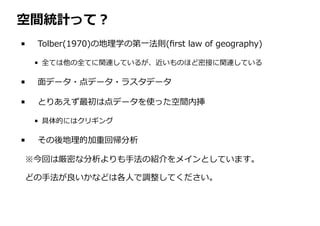
空間統計って︖ Tolber(1970)の地理学の第⼀法則(first law of
geography) 全ては他の全てに関連しているが、近いものほど密接に関連している ⾯データ・点データ・ラスタデータ とりあえず最初は点データを使った空間内挿 具体的にはクリギング その後地理的加重回帰分析 ※今回は厳密な分析よりも⼿法の紹介をメインとしています。 どの⼿法が良いかなどは各⼈で調整してください。
4.
sfパッケージ
5.
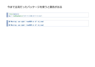
今まで主流だったパッケージを使うと警告が出る library(maptools) map <- readShapeSpatial("L01-17_13_GML/L01-17_13.shp") ##
Warning: use rgdal::readOGR or sf::st_read ## Warning: use rgdal::readOGR or sf::st_read
6.
sfパッケージで読み込み 国⼟数値情報の公⽰地価(H29)のデータ(point data)を⽤います。 library(sf) library(dplyr) #フォルダ名に日本語が入っていると使えないことが多い d <-
st_read(dsn = "L01-17_13_GML", layer = "L01-17_13",stringsAsFactors = FALSE) dat <- select(d, LPH = L01_006, CITY = L01_018, STATUS = L01_021) %>% mutate_at("LPH",as.integer) %>% filter(!CITY %in% c("神津島", "新島", "東京大島", "東京三宅", "八丈", "小笠原")) %>% filter(STATUS == "住宅") dat_mat <- t(matrix(unlist(dat$geometry), nrow=2)) dat$Y <- dat_mat[,2] dat$X <- dat_mat[,1] dat$ID <- 1:1360 dat2 <- as.data.frame(dat) sfのメリットの1つはdata frameのようにdplyrで操作できることです。
7.
plot(dat[1]) 今⽇はsfパッケージに挑戦し、割と挫折した話です。
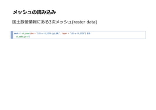
8.
メッシュの読み込み 国⼟数値情報にある3次メッシュ(raster data) mesh <-
st_read(dsn = "L03-a-14_5339-jgd_GML", layer = "L03-a-14_5339") %>% st_make_grid()
9.
ヴァリオグラムの計算
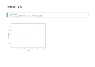
10.
定数項モデル library(gstat) plot(variogram(LPH/10000~1, locations=~X+Y, data=dat2))
11.
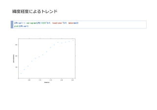
緯度経度によるトレンド LPH.var1 <- variogram(LPH/10000~X+Y,
locations=~X+Y, data=dat2) plot(LPH.var1)
12.
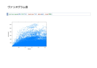
ヴァリオグラム雲 plot(variogram(LPH/10000~X+Y, locations=~X+Y, data=dat2,
cloud=TRUE))
13.
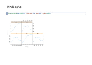
異⽅性モデル plot(variogram(LPH/10000~X+Y, locations=~X+Y, data=dat2,
alpha=0:4*90))
14.
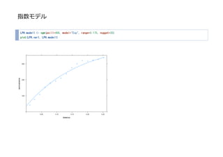
指数モデル LPH.model1 <- vgm(psill=400,
model="Exp", range=0.175, nugget=35) plot(LPH.var1, LPH.model1)
15.
空間内挿
16.
普遍型クリギング LPH.gu <- gstat(id="ID",
formula=LPH/10000~X+Y, locations=~X+Y, data=dat2, model=LPH.model1) #LPH.pu <- predict(LPH.gu, mesh) #spplot(LPH.pu[1]) sfc_POLYGONは使えないとエラーが出る
17.
sfパッケージを諦める mesh2 <- st_read(dsn
= "L03-a-14_5339-jgd_GML", layer = "L03-a-14_5339") %>% st_make_grid() %>% st_coordinates() mesh2 <- coordinates(mesh2)%>% as.data.frame() coordinates(mesh2) <- c("X","Y") mesh2 <- as(mesh2, "SpatialPixelsDataFrame") LPH.gu <- gstat(id="ID", formula=LPH/10000~X+Y, locations=~X+Y, data=dat2, model=LPH.model1) LPH.pu <- predict(LPH.gu, mesh2) ## [using universal kriging]
18.
推計結果 spplot(LPH.pu[1])
19.
誤差 spplot(LPH.pu[2])
20.
地理的加重回帰分析(GWR)
21.
できなかっただけで終わるのも寂しいので地理的加重回帰分析します。 国⼟数値情報より公⽰地価(H27)及び都道府県地価調査(H27)の平均 (円/m2)と国勢調査(H27)から夜間⼈⼝密度(⼈/km2)と第3次産業就業 ⼈⼝密度(⼈/km2)を⽤います。 library(spdep) library(spgwr) library(classInt) # データの読み込み poly <-
read_sf(dsn="chika", layer="kanto_area") %>% mutate_at(vars(c("N03_007")),as.integer) %>% filter(FIRST_N0_2 != "所属未定地") chika <- read.csv("chika/chika.csv",header = T) #データの結合 kanto <- left_join(poly, chika, by = c("N03_007" = "CODE")) %>% mutate(area = area / 1000000) %>% mutate(EMP3D = (EMP3) / area) %>% mutate(POPD = (POP) / area)
22.
隣接⾏列の作成 coords <- matrix(0,
nrow=length(kanto$LPH), ncol=2) coords[,1] <- kanto$X coords[,2] <- kanto$Y lph.tri.nb <- tri2nb(coords)
23.
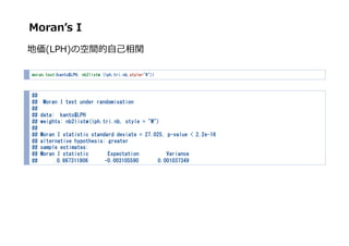
Moranʼs I 地価(LPH)の空間的⾃⼰相関 moran.test(kanto$LPH, nb2listw
(lph.tri.nb,style="W")) ## ## Moran I test under randomisation ## ## data: kanto$LPH ## weights: nb2listw(lph.tri.nb, style = "W") ## ## Moran I statistic standard deviate = 27.025, p-value < 2.2e-16 ## alternative hypothesis: greater ## sample estimates: ## Moran I statistic Expectation Variance ## 0.867311806 -0.003105590 0.001037349
24.
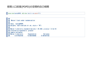
夜間⼈⼝密度(POPD)の空間的⾃⼰相関 moran.test(kanto$POPD, nb2listw (lph.tri.nb,style="W")) ## ##
Moran I test under randomisation ## ## data: kanto$POPD ## weights: nb2listw(lph.tri.nb, style = "W") ## ## Moran I statistic standard deviate = 25.484, p-value < 2.2e-16 ## alternative hypothesis: greater ## sample estimates: ## Moran I statistic Expectation Variance ## 0.817623729 -0.003105590 0.001037183
25.
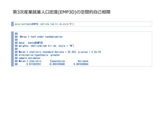
第3次産業就業⼈⼝密度(EMP3D)の空間的⾃⼰相関 moran.test(kanto$EMP3D, nb2listw (lph.tri.nb,style="W")) ## ##
Moran I test under randomisation ## ## data: kanto$EMP3D ## weights: nb2listw(lph.tri.nb, style = "W") ## ## Moran I statistic standard deviate = 25.323, p-value < 2.2e-16 ## alternative hypothesis: greater ## sample estimates: ## Moran I statistic Expectation Variance ## 0.811922251 -0.003105590 0.001035854
26.
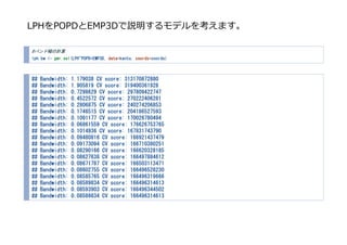
LPHをPOPDとEMP3Dで説明するモデルを考えます。 #バンド幅の計算 lph.bw <- gwr.sel(LPH~POPD+EMP3D,
data=kanto, coords=coords) ## Bandwidth: 1.179038 CV score: 313170872880 ## Bandwidth: 1.905819 CV score: 319400361928 ## Bandwidth: 0.7298629 CV score: 297809422747 ## Bandwidth: 0.4522572 CV score: 270222406281 ## Bandwidth: 0.2806875 CV score: 240274206853 ## Bandwidth: 0.1746515 CV score: 204186527593 ## Bandwidth: 0.1091177 CV score: 170026780494 ## Bandwidth: 0.06861559 CV score: 176626753765 ## Bandwidth: 0.1014936 CV score: 167831743790 ## Bandwidth: 0.09480816 CV score: 166921437479 ## Bandwidth: 0.09173094 CV score: 166710380251 ## Bandwidth: 0.08290166 CV score: 166620328185 ## Bandwidth: 0.08627638 CV score: 166497884612 ## Bandwidth: 0.08671787 CV score: 166503113471 ## Bandwidth: 0.08602755 CV score: 166496528230 ## Bandwidth: 0.08585765 CV score: 166496319666 ## Bandwidth: 0.08589834 CV score: 166496314613 ## Bandwidth: 0.08593903 CV score: 166496344502 ## Bandwidth: 0.08589834 CV score: 166496314613
27.
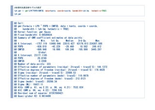
#地理的加重回帰モデルの推定 lph.gwr <- gwr(LPH~POPD+EMP3D,
data=kanto, coords=coords, bandwidth=lph.bw, hatmatrix=TRUE) lph.gwr ## Call: ## gwr(formula = LPH ~ POPD + EMP3D, data = kanto, coords = coords, ## bandwidth = lph.bw, hatmatrix = TRUE) ## Kernel function: gwr.Gauss ## Fixed bandwidth: 0.08589834 ## Summary of GWR coefficient estimates at data points: ## Min. 1st Qu. Median 3rd Qu. Max. ## X.Intercept. -1757.119 13468.046 23515.427 63176.813 224307.500 ## POPD -938.010 -42.229 -20.460 10.582 249.412 ## EMP3D -686.948 18.996 109.246 195.089 3445.297 ## Global ## X.Intercept. 23177.1185 ## POPD 20.8749 ## EMP3D 0.2208 ## Number of data points: 323 ## Effective number of parameters (residual: 2traceS - traceS'S): 144.1372 ## Effective degrees of freedom (residual: 2traceS - traceS'S): 178.8628 ## Sigma (residual: 2traceS - traceS'S): 22088.53 ## Effective number of parameters (model: traceS): 110.9879 ## Effective degrees of freedom (model: traceS): 212.0121 ## Sigma (model: traceS): 20288.34 ## Sigma (ML): 16437.11 ## AICc (GWR p. 61, eq 2.33; p. 96, eq. 4.21): 7532.024 ## AIC (GWR p. 96, eq. 4.22): 7298.536 ## Residual sum of squares: 87267699421 ## Quasi-global R2: 0.9614499
28.
結果を地図で表⽰
29.
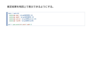
推定結果を地図上で表⽰できるようにする。 kanto <- kanto
%>% mutate(gwr.popd = lph.gwr$SDF$POPD) %>% mutate(gwr.emp3d = lph.gwr$SDF$EMP3D) %>% mutate(gwr.pred.se = lph.gwr$SDF$pred.se) %>% mutate(gwr.localR2 = lph.gwr$SDF$localR2) pal1 <- gray.colors(n=4,start=1,end=0.3)
30.
夜間⼈⼝密度の回帰係数 q_gwr <- classIntervals(round(kanto$gwr.popd,2),
n=4, style="quantile") q_gwr_Col <- findColours(q_gwr,pal1) plot(kanto[20],col=q_gwr_Col,main="") legend("bottomleft",fill=attr(q_gwr_Col,"palette"),legend=names(attr(q_gwr_Col,"table")), cex=1.1, bty="n")
31.
第3次産業就業⼈⼝の回帰係数 q_gwr <- classIntervals(round(kanto$gwr.emp3d,2),
n=4, style="quantile") q_gwr_Col <- findColours(q_gwr,pal1) plot(kanto[21],col=q_gwr_Col,main="") legend("bottomleft",fill=attr(q_gwr_Col,"palette"),legend=names(attr(q_gwr_Col,"table")), cex=1.1, bty="n")
32.
標準誤差 q_gwr.se <- classIntervals(round(kanto$gwr.pred.se,2),
n=4, style="quantile") q_gwr.se_Col <- findColours(q_gwr.se,pal1) plot(kanto[22],col=q_gwr.se_Col,main="") legend("bottomleft",fill=attr(q_gwr.se_Col,"palette"),legend=names(attr(q_gwr.se_Col,"table")), cex=1, bty="n")
33.
localR2 q_gwr.localR2 <- classIntervals(round(kanto$gwr.localR2,2),
n=4, style="quantile") q_gwr.localR2_Col <- findColours(q_gwr.localR2,pal1) plot(kanto[23],col=q_gwr.localR2_Col,main="") legend("bottomleft",fill=attr(q_gwr.localR2_Col,"palette"),legend=names(attr(q_gwr.localR2_Col,"table")), cex=1, bty="n")
34.
参考⽂献など Arbia, Giuseppe. 2016.
『Rで学ぶ空間計量経済学⼊⾨』. 勁草書房. 古⾕知之. 2011. 『Rによる空間データの統計分析』. 朝倉書店. 岩波データサイエンス刊⾏委員会. 2016. 『岩波データサイエンス vol.4 : 特集地理空間情報処理』. 岩波書店. 瀬⾕創 ・ 堤盛⼈. 2014. 『空間統計学 : ⾃然科学から⼈⽂・社会科学 まで』. 朝倉書店. ⾕村晋. 2010. 『地理空間データ分析』. 共⽴出版. Tobler, W. R. 1970. “A Computer Movie Simulating Urban Growth in the Detroit Region.” Economic Geography 46: 234–40. 堤盛⼈ ・ 村上⼤輔 ・ 嶋⽥章. 2014. 「我が国の三⼤都市圏を対象とし た住宅地価分布図の作成.」 『GIS-理論と応⽤』 22(2): 69–79.
35.
参考ホームページ(順不同) https://cran.r-project.org/web/packages/sf/vignettes/sf1.html http://notchained.hatenablog.com/entry/2017/01/06/213333 https://github.com/r-spatial/sf/wiki/migrating https://cran.r-project.org/web/views/Spatial.html http://web.sfc.keio.ac.jp/~maunz/wiki/index.php? Data%20Sciences%20for%20the%20Resilient%20Society
36.
ご清聴ありがとうございました
Download


![sfパッケージで読み込み
国⼟数値情報の公⽰地価(H29)のデータ(point data)を⽤います。
library(sf)
library(dplyr)
#フォルダ名に日本語が入っていると使えないことが多い
d <- st_read(dsn = "L01-17_13_GML", layer = "L01-17_13",stringsAsFactors = FALSE)
dat <- select(d, LPH = L01_006, CITY = L01_018, STATUS = L01_021) %>%
mutate_at("LPH",as.integer) %>%
filter(!CITY %in% c("神津島", "新島", "東京大島", "東京三宅", "八丈", "小笠原")) %>%
filter(STATUS == "住宅")
dat_mat <- t(matrix(unlist(dat$geometry), nrow=2))
dat$Y <- dat_mat[,2]
dat$X <- dat_mat[,1]
dat$ID <- 1:1360
dat2 <- as.data.frame(dat)
sfのメリットの1つはdata frameのようにdplyrで操作できることです。](https://image.slidesharecdn.com/random-170902075222/85/slide-6-320.jpg)
![plot(dat[1])
今⽇はsfパッケージに挑戦し、割と挫折した話です。](https://image.slidesharecdn.com/random-170902075222/85/slide-7-320.jpg)


![普遍型クリギング
LPH.gu <- gstat(id="ID", formula=LPH/10000~X+Y, locations=~X+Y, data=dat2, model=LPH.model1)
#LPH.pu <- predict(LPH.gu, mesh)
#spplot(LPH.pu[1])
sfc_POLYGONは使えないとエラーが出る](https://image.slidesharecdn.com/random-170902075222/85/slide-16-320.jpg)
![sfパッケージを諦める
mesh2 <- st_read(dsn = "L03-a-14_5339-jgd_GML", layer = "L03-a-14_5339") %>%
st_make_grid() %>%
st_coordinates()
mesh2 <- coordinates(mesh2)%>%
as.data.frame()
coordinates(mesh2) <- c("X","Y")
mesh2 <- as(mesh2, "SpatialPixelsDataFrame")
LPH.gu <- gstat(id="ID", formula=LPH/10000~X+Y, locations=~X+Y, data=dat2, model=LPH.model1)
LPH.pu <- predict(LPH.gu, mesh2)
## [using universal kriging]](https://image.slidesharecdn.com/random-170902075222/85/slide-17-320.jpg)
![推計結果
spplot(LPH.pu[1])](https://image.slidesharecdn.com/random-170902075222/85/slide-18-320.jpg)
![誤差
spplot(LPH.pu[2])](https://image.slidesharecdn.com/random-170902075222/85/slide-19-320.jpg)

![隣接⾏列の作成
coords <- matrix(0, nrow=length(kanto$LPH), ncol=2)
coords[,1] <- kanto$X
coords[,2] <- kanto$Y
lph.tri.nb <- tri2nb(coords)](https://image.slidesharecdn.com/random-170902075222/85/slide-22-320.jpg)

![夜間⼈⼝密度の回帰係数
q_gwr <- classIntervals(round(kanto$gwr.popd,2), n=4, style="quantile")
q_gwr_Col <- findColours(q_gwr,pal1)
plot(kanto[20],col=q_gwr_Col,main="")
legend("bottomleft",fill=attr(q_gwr_Col,"palette"),legend=names(attr(q_gwr_Col,"table")), cex=1.1, bty="n")](https://image.slidesharecdn.com/random-170902075222/85/slide-30-320.jpg)
![第3次産業就業⼈⼝の回帰係数
q_gwr <- classIntervals(round(kanto$gwr.emp3d,2), n=4, style="quantile")
q_gwr_Col <- findColours(q_gwr,pal1)
plot(kanto[21],col=q_gwr_Col,main="")
legend("bottomleft",fill=attr(q_gwr_Col,"palette"),legend=names(attr(q_gwr_Col,"table")), cex=1.1, bty="n")](https://image.slidesharecdn.com/random-170902075222/85/slide-31-320.jpg)
![標準誤差
q_gwr.se <- classIntervals(round(kanto$gwr.pred.se,2), n=4, style="quantile")
q_gwr.se_Col <- findColours(q_gwr.se,pal1)
plot(kanto[22],col=q_gwr.se_Col,main="")
legend("bottomleft",fill=attr(q_gwr.se_Col,"palette"),legend=names(attr(q_gwr.se_Col,"table")), cex=1, bty="n")](https://image.slidesharecdn.com/random-170902075222/85/slide-32-320.jpg)
![localR2
q_gwr.localR2 <- classIntervals(round(kanto$gwr.localR2,2), n=4, style="quantile")
q_gwr.localR2_Col <- findColours(q_gwr.localR2,pal1)
plot(kanto[23],col=q_gwr.localR2_Col,main="")
legend("bottomleft",fill=attr(q_gwr.localR2_Col,"palette"),legend=names(attr(q_gwr.localR2_Col,"table")), cex=1, bty="n")](https://image.slidesharecdn.com/random-170902075222/85/slide-33-320.jpg)