1. CCR Summer Proceedings 2015 1
SPPARKS SOFTWARE UPDATES
JUSTIN M. ROBERTS∗, JOHN A. MITCHELL†, AIDAN P. THOMPSON‡, AND VEENA
TIKARE§
Abstract. SPPARKS, an acronym for Stochastic Parallel Particle Kinetic Simulator, is a kinetic
Monte Carlo algorithm to simulate events such as grain growth and diffusion. Extensions of the
program have been written but not finished. Our work was to understand how SPPARKS operates
and add new functionality while providing documentation on how to use the new functionality. This
report outlines what was accomplished during the summer of 2015.
1. Introduction. After we learned how to compile and run SPPARKS, we were
able to start testing and writing documentation on new SPPARKS applications. This
sometimes required updating the new applications to the latest version of SPPARKS.
During the summer of 2015, we were able to completely finish one application and
made significant progress on another.
2. Understanding SPPARKS terminology. SPPARKS uses its own soft-
ware specific terminology to refer to particular data structures and operations. We
will explain some of the terminology here.
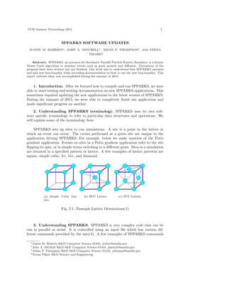
SPPARKS sets up sites to run simulations. A site is a point in the lattice at
which an event can occur. The events performed at a given site are unique to the
application driving SPPARKS. For example, below we make mention of the Potts
gradient application. Events on sites in a Potts gradient application refer to the site
flipping its spin, or in simple terms switching to a different grain. Sites in a simulation
are situated in a specified pattern or lattice. A few examples of lattice patterns are
square, simple cubic, fcc, bcc, and diamond.
(a) Simple Cubic Lat-
tice
(b) BCC Lattice (c) FCC Lattice
Fig. 2.1: Example Lattice Orientations(1)
3. Understanding SPPARKS. SPPARKS is very complex code that can be
run in parallel or serial. It is controlled using an input file which has various dif-
ferent commands provided by the user(3). A few examples of SPPARKS commands
∗Justin M. Roberts R&D Computer Science 01444, jrober@sandia.gov
†John A. Mitchell R&D S&E Computer Science 01444, jamitch@sandia.gov
‡Aidan P. Thompson R&D S&E Computer Science 01444, athomps@sandia.gov
§Veena Tikare R&D Science and Engineering

2. 2 SPPARKS computing
are sweep, lattice, solve style, app style, run, and diag style. These commands spec-
ify which SPPARKS application to use, which diagnostic tools to use, and how it is
solved. The input file is read with the parse function called from the file() function
within input.cpp. After it is parsed, the command is executed from a list of options
within the execute command() function within input.cpp. The iterate() function con-
trols which solver to use. The simulation can be solved by using either KMC (Kinetic
Monte Carlo) or rKMC (rejection Kinetic Monte Carlo). The iterate() function is
found from within app lattice.cpp and is called from run() found in app.cpp. The run
command specifies how many time steps the program will execute.
SPPARKS generates information from a simulation in various forms. Information
can come from the log file, dump images, dump files, and diagnostics. Diagnostics
can be chosen using the diag style command. We are currently working on a new
diag style command called curvature.
4. Curvature. The curvature diagnostic was originally developed by Veena
Tikare (vtikare@sandia.gov). The diagnostic computes curvatures for each grain and
then writes this information to disk for further analysis. It also has the option of
writing the number of grains to the log file at a given time step defined by the stats
command. The log file option was not originally part of the code but was added by
using the functions stats header() and stats(). These functions are called from stats()
and stats header() from output.cpp. An example of how a log file is output to the
screen during run time is given below. Notice that Ngrains is an additional column
provided by the curvature diagnostic Table 4.1.
Table 4.1: Command line output with Ngrains
Time Naccept Nreject Nsweeps CPU Energy Ngrains
0 0 0 0 0 406250 15625
2.5 93493 922132 65 0.518 127208 108
5.03846 109515 1937360 131 1.01 101282 51
7.53846 121225 2941275 196 1.49 89664 35
10.0385 132541 3945584 261 1.98 77620 24
12.5385 141994 4951756 326 2.45 69984 18
15.0385 151674 5957701 391 2.93 60976 15
17.5 162959 6946416 455 3.4 43178 9
20 171903 7953097 520 3.86 17004 2
22.5 172496 8968129 585 4.31 16600 2
25 172972 9983278 650 4.76 16600 2
Curvature Mv is defined as
Mv = edges 1/2βL,
where L is the length of each edge, and β is the angle formed by two faces on an edge.
After implementing the function into SPPARKS it becomes:

3. Justin M. Roberts, Aidan P. Thompson, John A. Mitchell, Veena Tikare 3
Mv = 1/2 ∗ π/2[Eo − Ei]L,
where Eo is the number of edges on a face which form an angle of π/2. Ei is the
number of edges on a face which form an angle of −π/2. Grain edges that share
three different grains and grain corners are not counted as part of the face curvature.
Therefore curvature is defined as face curvature.
The algorithm is still being tested but is very close to being added to the SP-
PARKS repository and included as a diagnostic option of SPPARKS.
5. Potts Gradient. Another application of SPPARKS we worked on and com-
pleted was an application called Potts gradient. The Potts model is typically used to
simulate grain growth in metals. Grain growth occurs when a metal is held at a high
temperature; at high temperature the metal undergoes recovery, recrystallization, and
nucleation.
The Potts gradient application adds temperature gradients to the Potts model.
Every site in the model is assigned a specific temperature. The temperature depends
linearly on its position in the lattice. The linear function is uniquely defined by the
value T0, at the center of the lattice, and gradients in the x,y, and z directions.
The equation
M0e−Q/KT
defines the mobility at each site where M0 is the mobility constant, K is Boltzmann’s
constant (8.6171e-5 eV/K), T is the temperature of the site, and Q is the activation
energy. The grain boundary mobility effects the probability that a particular grain
will grow. Higher mobility means higher probability of grain growth. The algorithm
was originally intended for use with temperature gradients, but we later added mo-
bility gradients as another option. When mobility gradients are used, each site is
assigned a mobility. The mobility is initialized at the center of the lattice and then
is assigned to each site depending on the site’s position in the lattice. The mobility
gradient is also defined as a linear function, analogous to the described above for
temperature.
The code was extensively tested and released with the SPPARKS source code.
Testing required image generation. A program was used to translate SPPARKS dump
files to paraview image files. Paraview enabled us to view grain growth animations.
With this tool we were able to uncover a critical bug in the code that was allowing
negative temperatures and mobilities to be assigned to certain sites. A simple error
check statement was added to resolve this issue.
Figure 5.1(a) demonstrates the mobility gradient option of the Potts gradient
model. As shown, grains on the left are much larger than the grains on the right.
This is because mobility on the left is significantly larger than mobility on the right.
To generate Figure 5.1(a), an initial mobility of 0.5 was chosen at the center
with lattice dimensions 400 X 100 X 100 giving a total of 4,000,000 sites oriented on
a simple cubic lattice. A mobility gradient of .0025 was defined in the X direction

4. 4 SPPARKS computing
(a) Potts model with mobility gradients applied
Fig. 5.1
which gives a mobility of 1.0 at x-max and 0 at x = 0. This example illustrates
the affect of mobility gradient on grain growth; a temperature gradient has a similar
effect(2). These parameters display the major changes that grain growth undergoes
when a mobility gradient is applied. We also generated videos of the simulation of
Figure 5.1(a) which are posted under the pictures and movies section on the SPPARKS
web site(3).
6. Understanding documentation. All of the HTML code on the SPPARKS
web site was generated from a text to HTML converter. The converter uses markup
commands to convert .txt files into HTML code that is read by a browser. The markup
commands include some but not all of the options of HTML. It includes elements such
as input, br, p, hr, a, ul, li, and pre. We learned how to write markup files and convert
them into HTML for the SPPARKS website. We wrote documentation for the new
Potts gradient application mentioned above which required updates to existing pages
and a whole new doc page. The formating style needed to be consistent with other
doc pages and needed careful consideration.
7. Conclusions. We were able to implement new applications into the existing
SPPARKS code along with documentation provided on the SPPARKS website(3).
This required us to learn how SPPARKS operates and how to write markup code. It
also required and a sound understanding of material science, and computer science.
More applications are in process and will be added to the SPPARKS source code and
doc pages in the near future.

5. Justin M. Roberts, Aidan P. Thompson, John A. Mitchell, Veena Tikare 5
References.
[1] H. Foll, Lattice and crystal. http://www.tf.uni-kiel.de/matwis/amat/def_
en/kap_1/basics/b1_3_1.html.
[2] J. A. Mitchell and V. Tikare, Numerical simulation of ni grain growth in a
thermal gradient, SIAM Conference on Computational Science and Engineering,
Salt Lake City, Utah, USA, 2015, Sandia Technical Report: SAND2015-1665c.
[3] S. Plimpton, C. Battaile, M. Chandross, L. Holm, A. Thompson,
V. Tikare, G. Wagner, E. Webb, X. Zhou, C. G. Cardona, and A. Sle-
poy, Spparks kinetic monte carlo simulator. http://spparks.sandia.gov/
index.html.
[4] , Crossing the Mesoscale No-Man’s Land via Parallel Kinetic Monte Carlo,
Sandia report SAND2009-6226, October 2009.