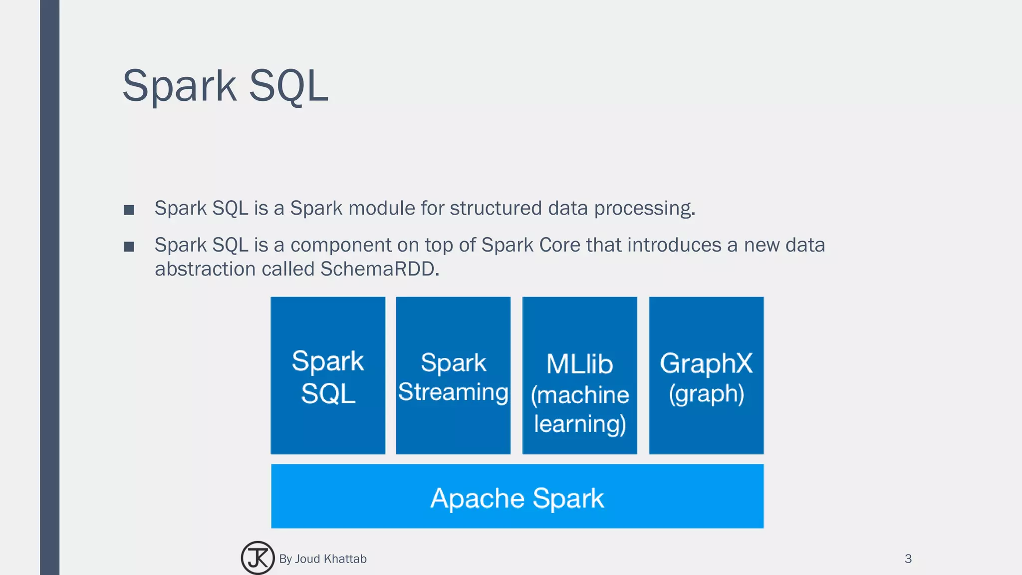
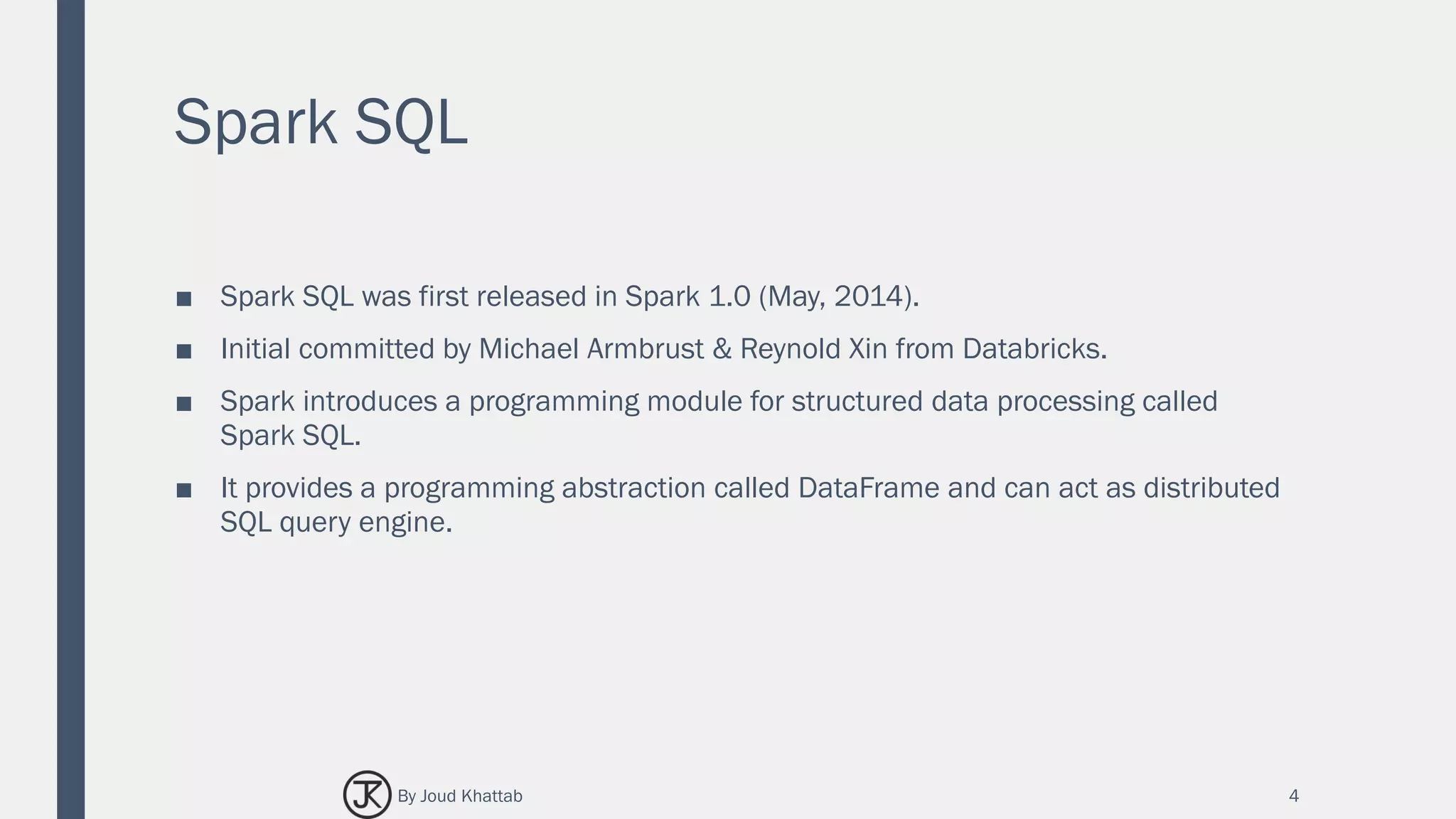
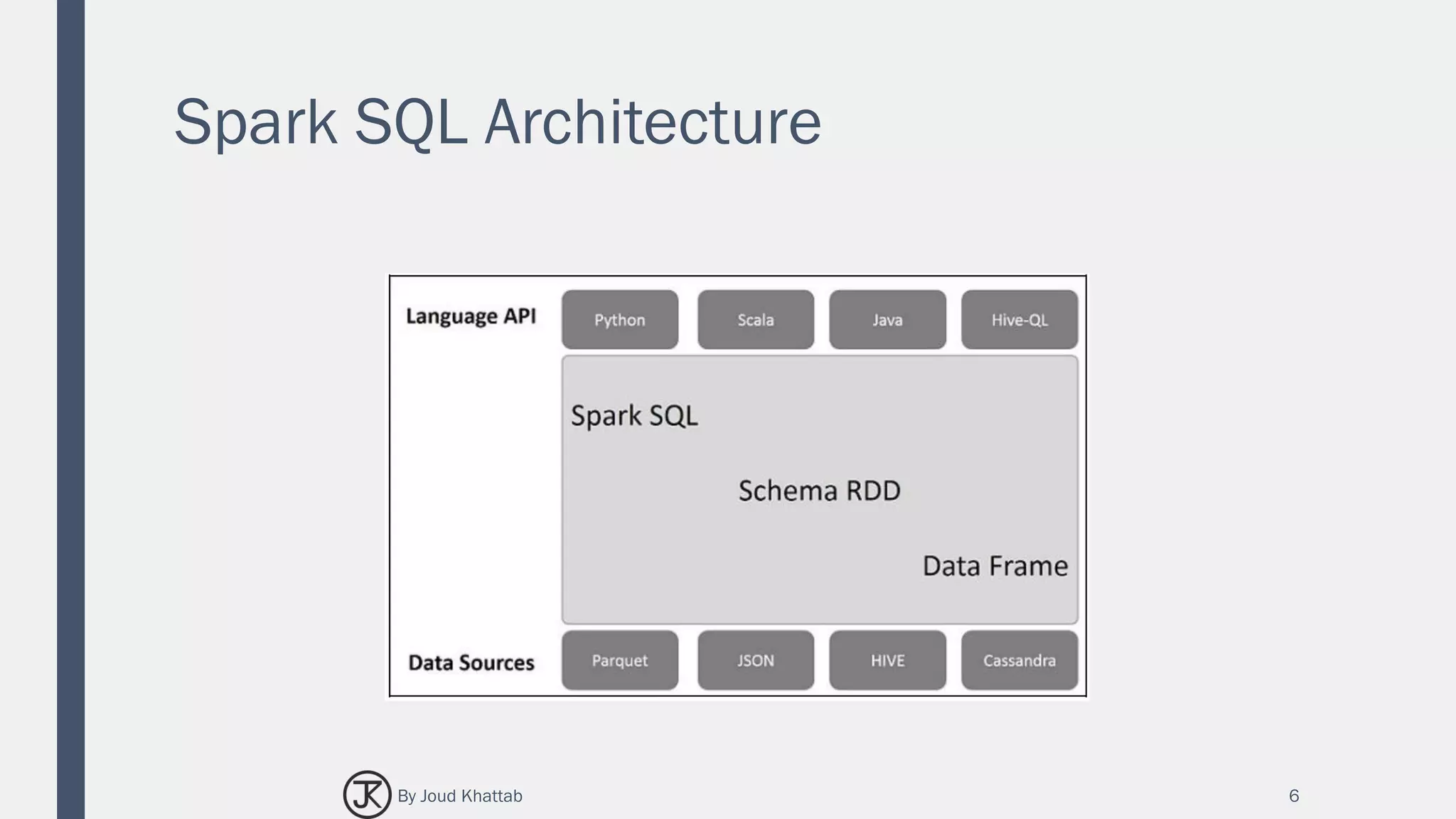
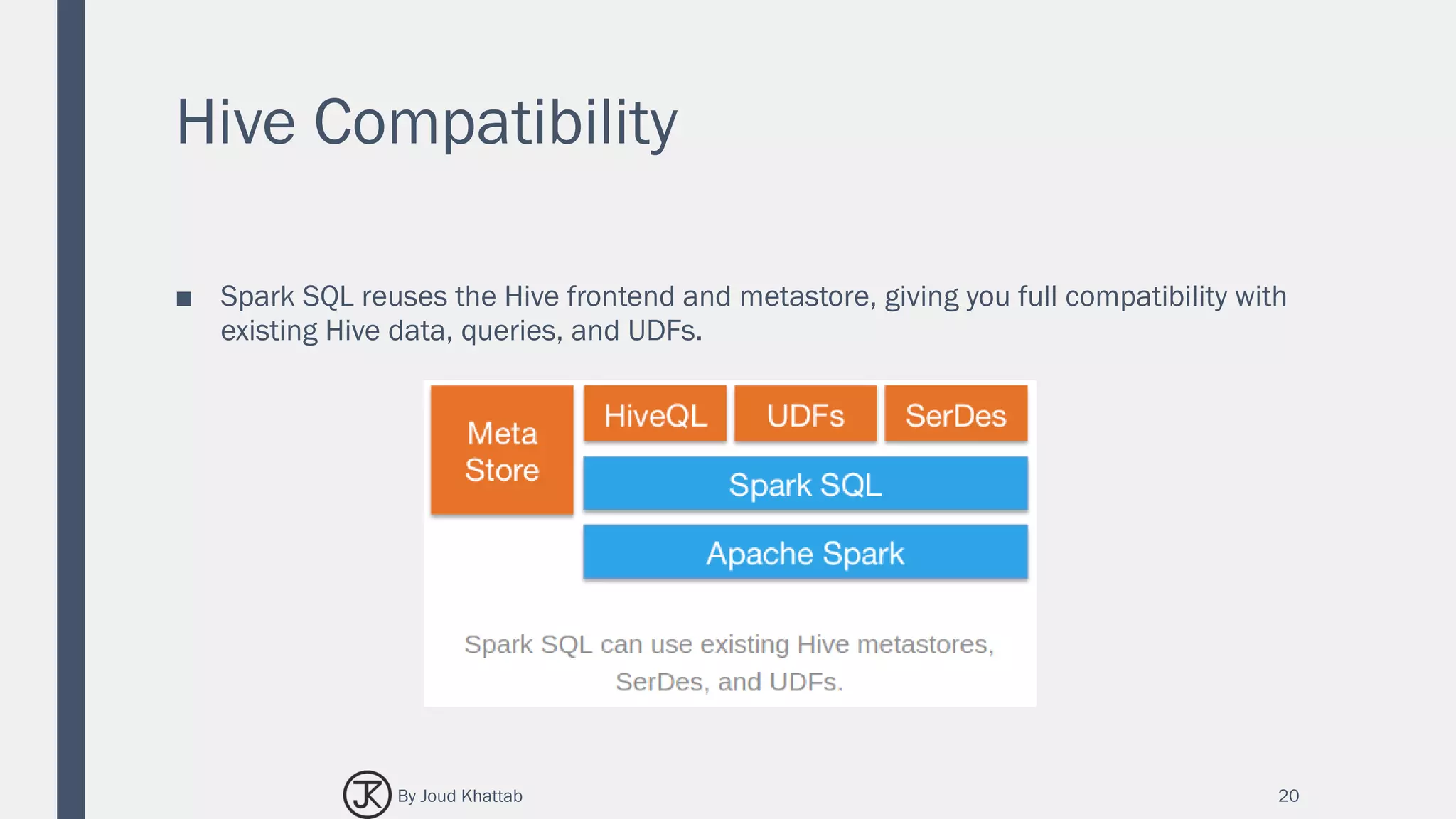
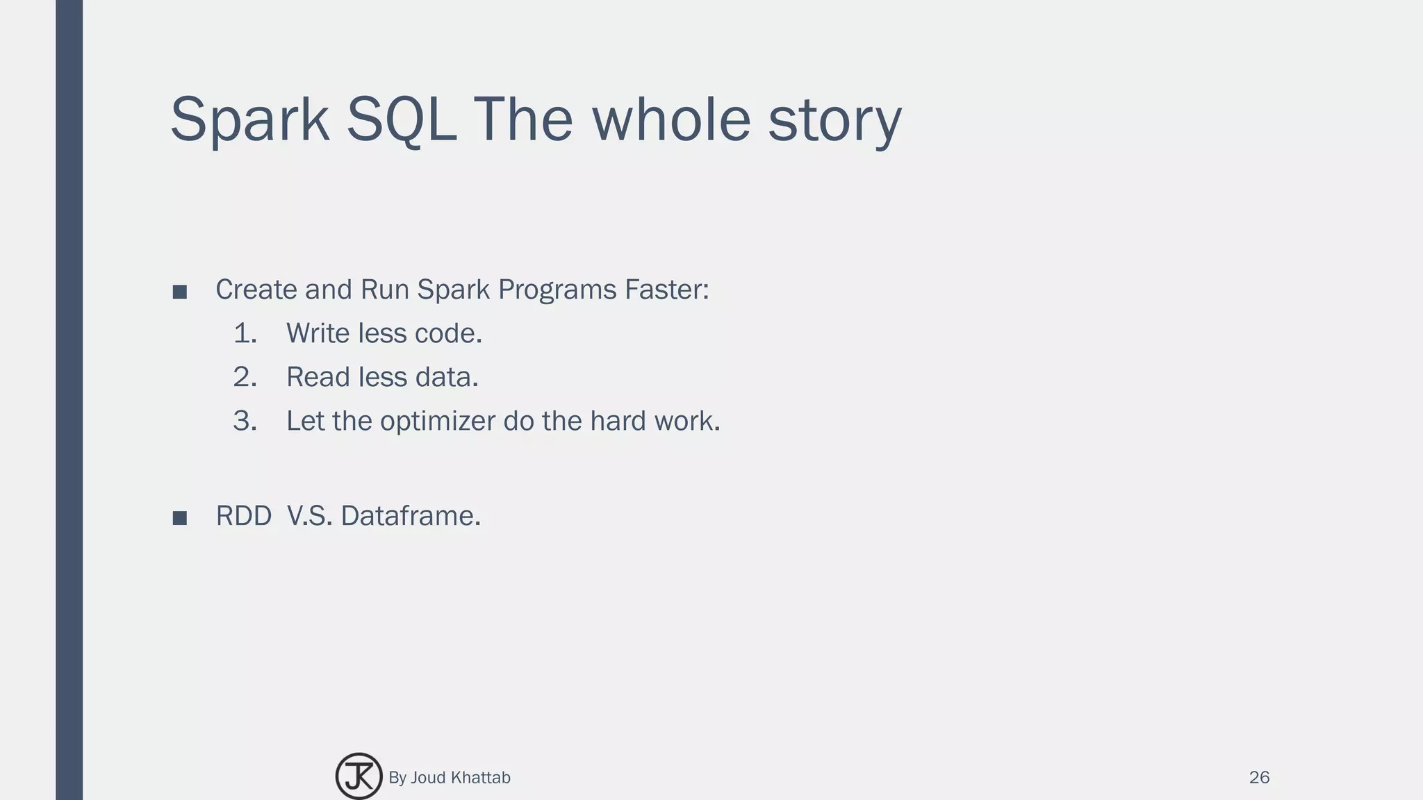
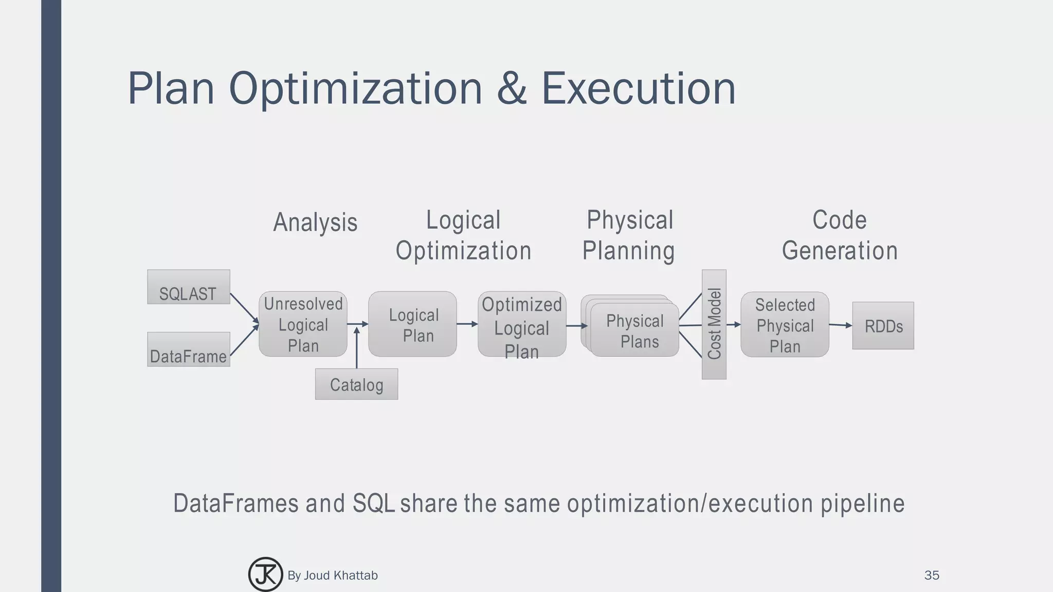
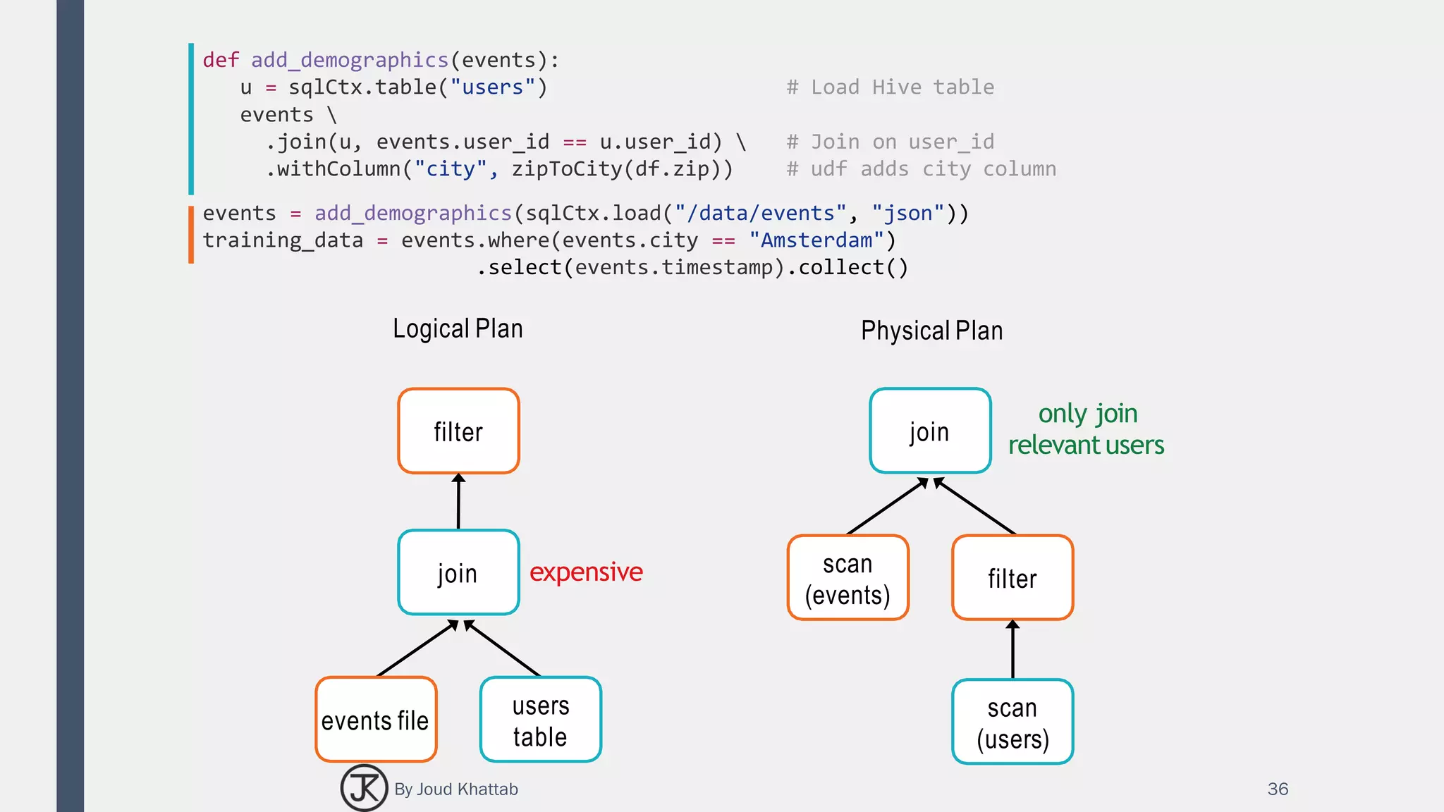
The document summarizes Spark SQL, which is a Spark module for structured data processing. It introduces key concepts like RDDs, DataFrames, and interacting with data sources. The architecture of Spark SQL is explained, including how it works with different languages and data sources through its schema RDD abstraction. Features of Spark SQL are covered such as its integration with Spark programs, unified data access, compatibility with Hive, and standard connectivity.

1. SPARK SQL
By
Eng. Joud Khattab

2. Content
1. Introduction.
2. Conceptual concepts:
– RDD, Dataset and DataFrame, Hive Database.
3. Spark SQL The whole story.
4. How does it all work?
5. Spark in R:
– Sparklyr Library.
6. Example.
7. References.
2By Joud Khattab

3. Spark SQL
■ Spark SQL is a Spark module for structured data processing.
■ Spark SQL is a component on top of Spark Core that introduces a new data
abstraction called SchemaRDD.
3By Joud Khattab

4. Spark SQL
■ Spark SQL was first released in Spark 1.0 (May, 2014).
■ Initial committed by Michael Armbrust & Reynold Xin from Databricks.
■ Spark introduces a programming module for structured data processing called
Spark SQL.
■ It provides a programming abstraction called DataFrame and can act as distributed
SQL query engine.
4By Joud Khattab

5. Challenges and Solutions
Challenges
■ Perform ETL to and from various
(semi- or unstructured) data sources.
■ Perform advanced analytics (e.g.
machine learning, graph processing)
that are hard to express in relational
systems.
Solutions
■ A DataFrame API that can perform
relational operations on both external
data sources and Spark’s built-in RDDs.
■ A highly extensible optimizer, Catalyst,
that uses features of Scala to add
composable rule, control code gen., and
define extensions.
5By Joud Khattab

6. Spark SQL Architecture
6By Joud Khattab

7. Spark SQL Architecture
■ Language API:
– Spark is compatible with different languages and Spark SQL.
– It is also, supported by these languages- API (python, scala, java, HiveQL).
■ Schema RDD:
– Spark Core is designed with special data structure called RDD.
– Generally, Spark SQL works on schemas, tables, and records.
– Therefore, we can use the Schema RDD as temporary table.
– We can call this Schema RDD as Data Frame.
■ Data Sources:
– Usually the Data source for spark-core is a text file, Avro file, etc. However, the Data
Sources for Spark SQL is different.
– Those are Parquet file, JSON document, HIVE tables, and Cassandra database.
7By Joud Khattab

8. Features of Spark SQL
1. Integrated:
– Seamlessly mix SQL queries with Spark programs.
– Spark SQL lets you query structured data as a distributed dataset (RDD) in
Spark, with integrated APIs in Python, Scala and Java.
– This tight integration makes it easy to run SQL queries alongside complex
analytic algorithms.
2. Unified Data Access:
– Load and query data from a variety of sources.
– Schema-RDDs provide a single interface for efficiently working with structured
data, including Apache Hive tables, parquet files and JSON files.
8By Joud Khattab

9. Features of Spark SQL
3. Hive Compatibility:
– Run unmodified Hive queries on existing warehouses.
– Spark SQL reuses the Hive frontend and MetaStore, giving you full compatibility
with existing Hive data, queries, and UDFs.
– Simply install it alongside Hive.
9
SELECT
COUNT(*)
FROM
hiveTable
WHERE
hive_udf(data)
By Joud Khattab

10. Features of Spark SQL
4. Standard Connectivity:
– Connect through JDBC or ODBC.
– Spark SQL includes a server mode with industry standard JDBC and ODBC
connectivity.
10By Joud Khattab

11. Features of Spark SQL
5. Scalability:
– Use the same engine for both interactive and long queries.
– Spark SQL takes advantage of the RDD model to support mid-query fault
tolerance, letting it scale to large jobs too.
– Do not worry about using a different engine for historical data.
11By Joud Khattab

12. SPARK RDD
Resilient Distributed Datasets
12By Joud Khattab

13. SPARK RDD
(Resilient Distributed Datasets)
■ RDD is a fundamental data structure of Spark.
■ It is an immutable distributed collection of objects that can be stored in memory or
disk across a cluster.
■ Each dataset in RDD is divided into logical partitions, which may be computed on
different nodes of the cluster.
■ Parallel functional transformations (map, filter, …).
■ Automatically rebuilt on failure.
■ RDDs can contain any type of Python, Java, or Scala objects, including user-defined
classes.
13By Joud Khattab

14. SPARK RDD
(Resilient Distributed Datasets)
■ Formally, an RDD is a read-only, partitioned collection of records.
■ RDDs can be created through deterministic operations on either data on stable
storage or other RDDs.
■ RDD is a fault-tolerant collection of elements that can be operated on in parallel.
■ There are two ways to create RDDs:
– parallelizing an existing collection in your driver program.
– referencing a dataset in an external storage system, such as a shared file
system, HDFS, HBase, or any data source offering a Hadoop Input Format.
■ Spark makes use of the concept of RDD to achieve faster and efficient MapReduce
operations. Let us first discuss how MapReduce operations take place and why they
are not so efficient.
14By Joud Khattab

15. SPARK SQL
DATASET AND DATAFRAME
15By Joud Khattab

16. Dataset and DataFrame
■ A distributed collection of data, which is organized into named columns.
■ Conceptually, it is equivalent to relational tables with good optimization techniques.
■ A DataFrame can be constructed from an array of different sources such as Hive
tables, Structured Data files, external databases, or existing RDDs.
■ This API was designed for modern Big Data and data science applications taking
inspiration from DataFrame in R Programming and Pandas in Python.
16By Joud Khattab

17. Dataset and DataFrame
■ DataFrame
– Data is organized into named columns, like a table in a relational database
■ Dataset: a distributed collection of data
– A new interface added in Spark 1.6
– Static-typing and runtime type-safety
17By Joud Khattab

18. Features of DataFrame
■ Ability to process the data in the size of Kilobytes to Petabytes on a single node
cluster to large cluster.
■ Supports different data formats (Avro, csv, elastic search, and Cassandra) and
storage systems (HDFS, HIVE tables, mysql, etc).
■ State of art optimization and code generation through the Spark SQL Catalyst
optimizer (tree transformation framework).
■ Can be easily integrated with all Big Data tools and frameworks via Spark-Core.
■ Provides API for Python, Java, Scala, and R Programming.
18By Joud Khattab

19. SPARK SQL & HIVE
19By Joud Khattab

20. Hive Compatibility
■ Spark SQL reuses the Hive frontend and metastore, giving you full compatibility with
existing Hive data, queries, and UDFs.
20By Joud Khattab

21. Hive
■ A database/data warehouse on top of Hadoop
– Rich data types
– Efficient implementations of SQL on top of map reduce
■ Support Analysis of large datasets stored in Hadoop's HDFS and compatible file
systems
– Such as Amazon S3 filesystem.
■ Provides an SQL-like language called HiveQL with schema.
21By Joud Khattab

22. Hive Architecture
■ User issues SQL query
■ Hive parses and plans query
■ Query converted to Map-Reduce
■ Map-Reduce runs by Hadoop
22By Joud Khattab

23. User-Defined Functions
■ UDF: Plug in your own processing code and invoke it from a Hive query
– UDF (Plain UDF)
■ Input: single row, Output: single row
– UDAF (User-Defined Aggregate Function)
■ Input: multiple rows, Output: single row
■ e.g. COUNT and MAX
– UDTF (User-Defined Table-generating Function)
■ Input: single row, Output: multiple rows
23By Joud Khattab

24. SPARK SQL
THE WHOLE STORY
24By Joud Khattab

25. The not-so-secret truth…
25
SQL
is not about SQL.
Decelerative Programing
By Joud Khattab

26. Spark SQL The whole story
■ Create and Run Spark Programs Faster:
1. Write less code.
2. Read less data.
3. Let the optimizer do the hard work.
■ RDD V.S. Dataframe.
26By Joud Khattab

27. Write Less Code:
Input & Output
■ Unified interface to reading/writing data in a variety of formats:
27
df = sqlContext.read
.format("json")
.option("samplingRatio", "0.1")
.load("/home/michael/data.json")
df.write
.format("parquet")
.mode("append")
.partitionBy("year")
.saveAsTable("fasterData")
read and write
functions create
new builders for
doing I/O
By Joud Khattab

28. Write Less Code:
Input & Output
■ Unified interface to reading/writing data in a variety of formats:
28
df = sqlContext.read
.format("json")
.option("samplingRatio", "0.1")
.load("/home/michael/data.json")
df.write
.format("parquet")
.mode("append")
.partitionBy("year")
.saveAsTable("fasterData")
Builder methods
are used to specify:
• Format
• Partitioning
• Handling of
existing data
• and more
By Joud Khattab

29. Write Less Code:
Input & Output
■ Unified interface to reading/writing data in a variety of formats:
29
df = sqlContext.read
.format("json")
.option("samplingRatio", "0.1")
.load("/home/michael/data.json")
df.write
.format("parquet")
.mode("append")
.partitionBy("year")
.saveAsTable("fasterData")
load(…), save(…) or
saveAsTable(…)
functions create
new builders for
doing I/O
By Joud Khattab

30. Read Less Data:
Efficient Formats
■ Parquet is an efficient columnar storage format:
– Compact binary encoding with intelligent compression (delta, RLE, etc).
– Each column stored separately with an index that allows skipping of unread
columns.
– Data skipping using statistics (column min/max, etc).
30By Joud Khattab

31. Write Less Code:
Powerful Operations
■ Common operations can be expressed concisely as calls to the DataFrame API:
– Selecting required columns.
– Joining different data sources.
– Aggregation (count, sum, average, etc).
– Filtering.
– Plotting results.
31By Joud Khattab

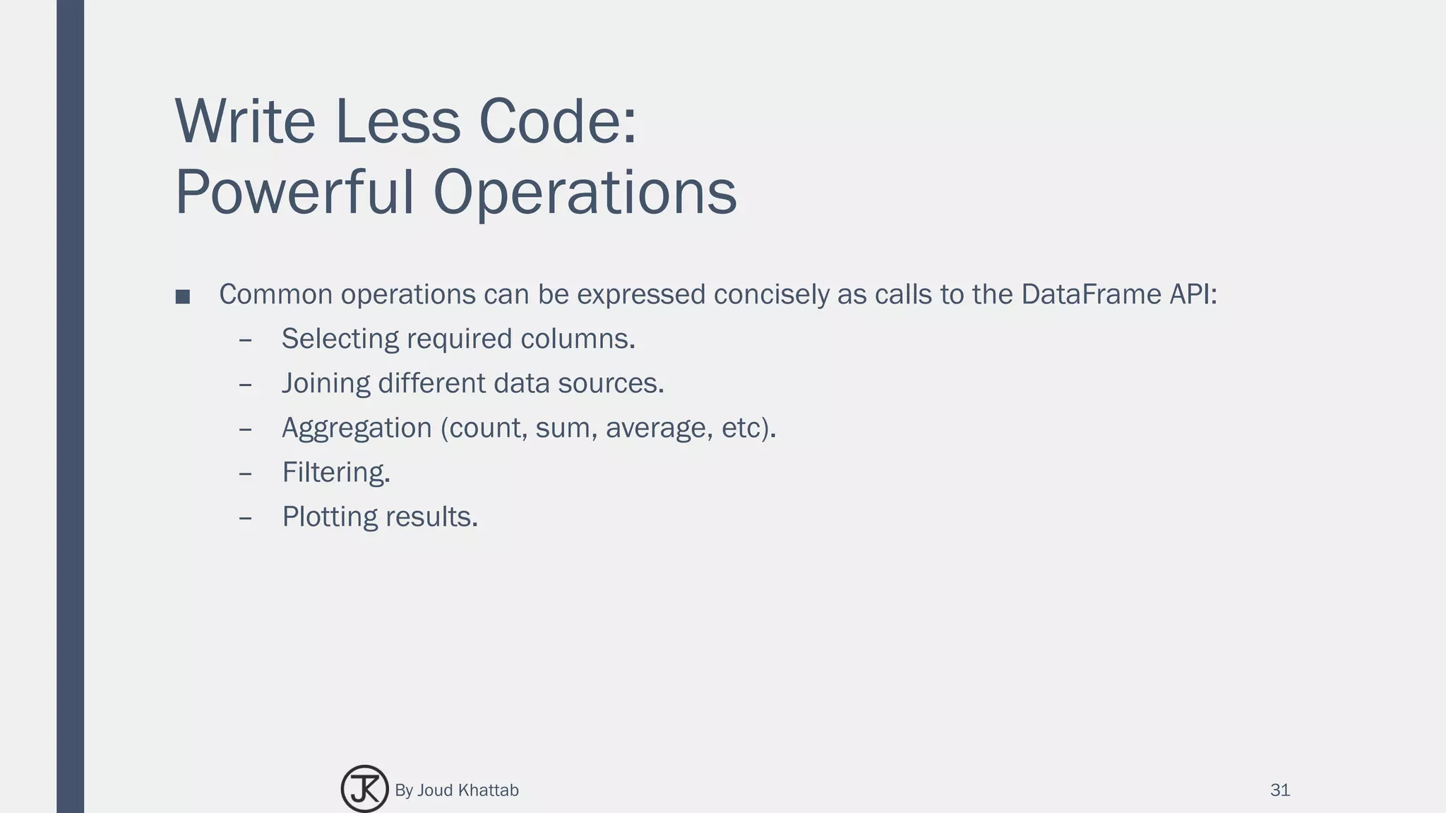
32. Write Less Code:
Compute an Average
32
private IntWritable one = new IntWritable(1)
private IntWritable output = new IntWritable()
proctected void map( LongWritable key,
Text value, Context context) {
String[] fields = value.split("t")
output.set(Integer.parseInt(fields[1]))
context.write(one, output)
}
IntWritable one = new IntWritable(1) DoubleWritable average
= new DoubleWritable()
protected void reduce( IntWritable key,
Iterable<IntWritable> values, Context
context) {
int sum = 0 int count = 0
for(IntWritable value : values) { sum +=
value.get()
count++
}
average.set(sum / (double) count)
context.Write(key, average)
data = sc.textFile(...).split("t")
data.map(lambda x: (x[0], [x.[1], 1]))
.reduceByKey(lambda x, y: [x[0] + y[0], x[1] + y[1]])
.map(lambda x: [x[0], x[1][0] / x[1][1]])
.collect()
By Joud Khattab

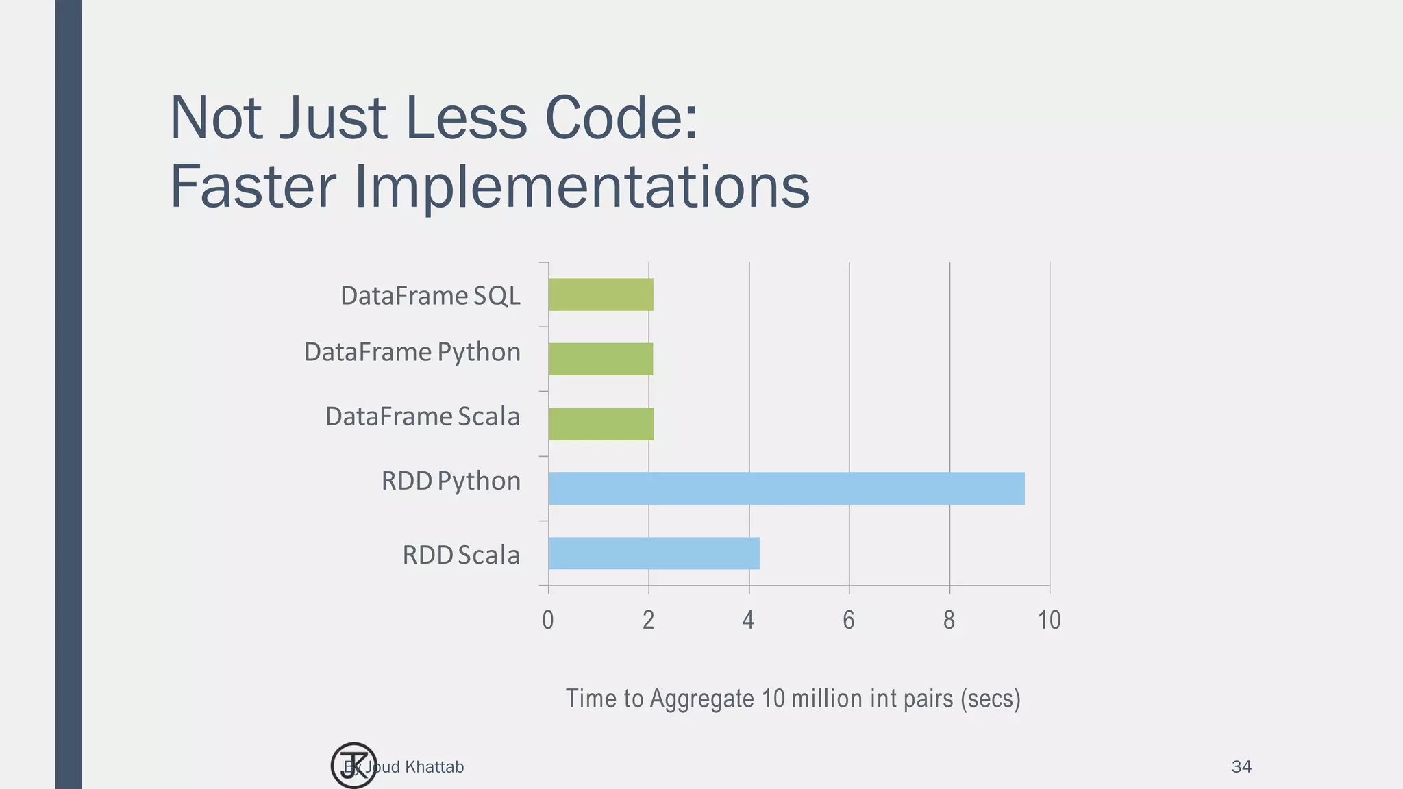
33. Write Less Code:
Compute an Average
33
Using RDDs
data = sc.textFile(...).split("t")
data.map(lambda x: (x[0], [int(x[1]), 1]))
.reduceByKey(lambda x, y: [x[0] + y[0], x[1] + y[1]])
.map(lambda x: [x[0], x[1][0] / x[1][1]])
.collect()
Using DataFrames
sqlCtx.table("people")
.groupBy("name")
.agg("name", avg("age"))
.collect()
Using SQL
SELECT name, avg(age)
FROM people
GROUP BY name
By Joud Khattab

34. Not Just Less Code:
Faster Implementations
34
0 2 4 6 8 10
DataFrameSQL
DataFramePython
DataFrameScala
RDDPython
RDDScala
Time to Aggregate 10 million int pairs (secs)
By Joud Khattab

35. Plan Optimization & Execution
35
SQLAST
DataFrame
Unresolved
Logical
Plan
Logical
Plan
Optimized
Logical
Plan
RDDs
Selected
Physical
Plan
Analysis Logical
Optimization
Physical
Planning
CostModel
Physical
Plans
Catalog
DataFrames and SQL share the same optimization/execution pipeline
Code
Generation
By Joud Khattab

36. 36
def add_demographics(events):
u = sqlCtx.table("users") # Load Hive table
events
.join(u, events.user_id == u.user_id) # Join on user_id
.withColumn("city", zipToCity(df.zip)) # udf adds city column
events = add_demographics(sqlCtx.load("/data/events", "json"))
training_data = events.where(events.city == "Amsterdam")
.select(events.timestamp).collect()
Logical Plan
filter
join
events file
users
table
expensive
only join
relevantusers
Physical Plan
join
scan
(events)
filter
scan
(users)
By Joud Khattab

37. HOW DOES IT ALL WORK?
37By Joud Khattab

38. An example query
SELECT name
FROM (
SELECT id, name
FROM People) p
WHERE p.id = 1
38
Logical
Plan
Project
name
Filter
id = 1
Project
id,name
People
By Joud Khattab

39. Naïve Query Planning
SELECT name
FROM (
SELECT id, name
FROM People) p
WHERE p.id = 1
39
Logical
Plan
Project
name
Filter
id = 1
Project
id,name
People
Physical
Plan
Project
name
Filter
id = 1
Project
id,name
TableScan
People
By Joud Khattab

40. Optimized Execution
■ Writing imperative code to optimize all
possible patterns is hard.
■ Instead write simple rules:
– Each rule makes one change
– Run many rules together to fixed
point.
40
IndexLookup
id = 1
return: name
Physical
Plan
Logical
Plan
Project
name
Filter
id = 1
Project
id,name
People
By Joud Khattab

41. Writing Rules as Tree Transformations
1. Find filters on top of projections.
2. Check that the filter can be evaluated
without the result of the project.
3. If so, switch the operators.
41
Project
name
Project
id,name
Filter
id = 1
People
Original
Plan
Project
name
Project
id,name
Filter
id = 1
People
Filter
Push-Down
By Joud Khattab

42. Optimizing with Rules
42
Project
name
Project
id,name
Filter
id = 1
People
Original
Plan
Project
name
Project
id,name
Filter
id = 1
People
Filter
Push-Down
Project
name
Filter
id = 1
People
Combine
Projection
IndexLookup
id = 1
return: name
Physical
Plan
By Joud Khattab

43. SPARKLYR
R interface for Apache Spark
43By Joud Khattab

44. Sparklyr
■ Founded on September 2016.
■ Connect to Spark from R.
■ Provides a complete dplyr backend.
■ Filter and aggregate Spark datasets
then bring them into R for analysis and
visualization.
■ Use Sparks distributed machine
learning library from R.
44By Joud Khattab

45. Manipulating Data with dplyr
■ dplyr is an R package for working with structured data both in and outside of R.
■ dplyr makes data manipulation for R users easy, consistent, and performant.
■ With dplyr as an interface to manipulating Spark DataFrames, you can:
– Select, filter, and aggregate data.
– Use window functions (e.g. for sampling).
– Perform joins on DataFrames.
– Collect data from Spark into R.
45By Joud Khattab

46. Reading Data
■ You can read data into Spark DataFrames using the following functions:
– Spark_read_csv.
– Spark_read_json.
– Spark_read_parquet.
■ Regardless of the format of your data, Spark supports reading data from a variety of
different data sources. These include data stored on HDFS, Amazon S3, or local files
available to the spark worker nodes.
■ Each of these functions returns a reference to a Spark DataFrame which can be
used as a dplyr table.
46By Joud Khattab

47. Flights Data
■ This guide will demonstrate some of the basic data manipulation verbs of dplyr by
using data from the nycflights13 R package.
■ This package contains data for all 336,776 flights departing New York City in 2013.
It also includes useful metadata on airlines, airports, weather, and planes.
■ Connect to the cluster and copy the flights data using the copy_to function.
■ Note:
– The flight data in nycflights13 is convenient for dplyr demonstrations because it
is small, but in practice large data should rarely be copied directly from R
objects.
47By Joud Khattab

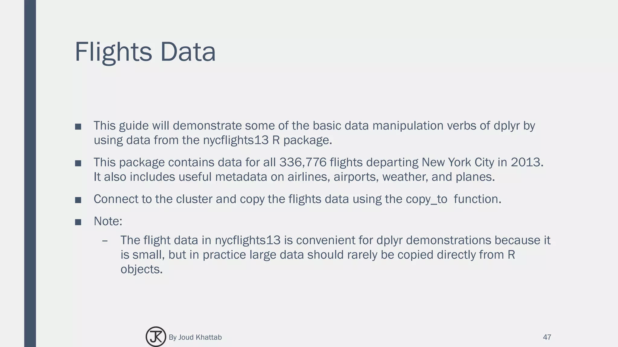
48. Flights Data
library(sparklyr)
library(dplyr)
library(nycflights13)
library(ggplot2)
sc <- spark_connect(master="local")
flights <- copy_to(sc, flights, "flights")
airlines <- copy_to(sc, airlines, "airlines")
src_tbls(sc)
[1] "airlines" "flights"
48By Joud Khattab

49. dplyr Verbs
■ Verbs are dplyr commands for manipulating data.
■ When connected to a Spark DataFrame, dplyr translates the commands into Spark
SQL statements.
■ Remote data sources use exactly the same five verbs as local data sources.
■ Here are the five verbs with their corresponding SQL commands:
– Select ~ select
– Filter ~ where
– Arrange ~ order
– Summarise ~ aggregators: sum, min, sd, etc.
– Mutate ~ operators: +. *, log, etc.
49By Joud Khattab

50. dplyr Verbs:
select
select(flights, year:day, arr_delay,
dep_delay)
# Source: lazy query [?? x 5]
# Database: spark_connection
year month day arr_delay dep_delay
<int> <int> <int> <dbl> <dbl>
1 2013 1 1 11 2
2 2013 1 1 20 4
3 2013 1 1 33 2
4 2013 1 1 -18 -1
5 2013 1 1 -25 -6
6 2013 1 1 12 -4
7 2013 1 1 19 -5
8 2013 1 1 -14 -3
9 2013 1 1 -8 -3
10 2013 1 1 8 -2
# ... with 3.368e+05 more rows
50By Joud Khattab

51. dplyr Verbs:
filter
filter(flights, dep_delay > 1000) # Source: lazy query [?? x 19]
# Database: spark_connection
year month day dep_time sched_dep_time dep_delay
<int> <int> <int> <int> <int> <dbl>
1 2013 1 9 641 900 1301
2 2013 1 10 1121 1635 1126
3 2013 6 15 1432 1935 1137
4 2013 7 22 845 1600 1005
5 2013 9 20 1139 1845 1014
# ... with 13 more variables: arr_time <int>, sched_arr_time
# <int>, arr_delay <dbl>, carrier <chr>, flight <int>, talinum
# <chr>, origin <chr>, dest <chr>, air_time <dbl>, distance
# <dbl>, hour <dbl>, minute <dbl>, time_hour <dbl>
51By Joud Khattab

52. dplyr Verbs:
arrange
arrange(flights, desc(dep_delay)) # Source: table<flights> [?? x 19]
# Database: spark_connection
# Ordered by: desc(dep_delay)
year month day dep_time sched_dep_time dep_delay
<int> <int> <int> <int> <int> <dbl>
1 2013 1 9 641 900 1301
2 2013 6 15 1432 1935 1137
3 2013 1 10 1121 1635 1126
4 2013 9 20 1139 1845 1014
5 2013 7 22 845 1600 1005
6 2013 4 10 1100 1900 960
7 2013 3 17 2321 810 911
8 2013 6 27 959 1900 899
9 2013 7 22 2257 759 898
10 2013 12 5 756 1700 896
# ... With 3.368e+05 more rows, and 13 more variables:
# arr_time <int>, sched_arr_time <int>, arr_delay <dbl>,
# carrier <chr>, flight <int>, tailnum <chr>, origin <chr>, dest
# <chr>, air_time <dbl>, distance <dbl>, hour <dbl>, minute
# <dbl>, time_hour <dbl>
52By Joud Khattab

53. dplyr Verbs:
summarise
summarise(flights, mean_dep_delay =
mean(dep_delay))
# Source: lazy query [?? x 1]
# Database: spark_connection
mean_dep_delay
<dbl>
1 12.63907
53By Joud Khattab

54. dplyr Verbs:
mutate
mutate(flights, speed = distance /
air_time * 60)
Source: query [3.368e+05 x 4]
Database: spark connection master=local[4]
app=sparklyr local=TRUE
# A tibble: 3.368e+05 x 4
year month day speed
<int> <int> <int> <dbl>
1 2013 1 1 370.0441
2 2013 1 1 374.2731
3 2013 1 1 408.3750
4 2013 1 1 516.7213
5 2013 1 1 394.1379
6 2013 1 1 287.6000
7 2013 1 1 404.4304
8 2013 1 1 259.2453
9 2013 1 1 404.5714
10 2013 1 1 318.6957
# ... with 3.368e+05 more rows
54By Joud Khattab

55. Laziness
■ When working with databases, dplyr tries to be as lazy as possible:
– It never pulls data into R unless you explicitly ask for it.
– It delays doing any work until the last possible moment: it collects together
everything you want to do and then sends it to the database in one step.
■ For example, take the following code:
– c1 <- filter(flights, day == 17, month == 5, carrier %in% c('UA', 'WN', 'AA', 'DL’))
– c2 <- select(c1, year, month, day, carrier, dep_delay, air_time, distance)
– c3 <- arrange(c2, year, month, day, carrier)
– c4 <- mutate(c3, air_time_hours = air_time / 60)
55By Joud Khattab

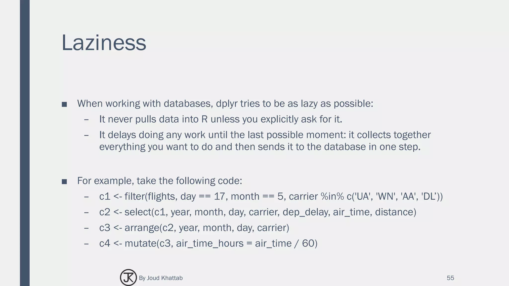
56. Laziness
■ This sequence of operations never
actually touches the database.
■ It’s not until you ask for the data (e.g.
by printing c4) that dplyr requests the
results from the database.
# Source: lazy query [?? x 20]
# Database: spark_connection
year month day carrier dep_delay air_time distance air_time_hours
<int> <int> <int> <chr> <dbl> <dbl> <dbl> <dbl>
1 2013 5 17 AA -2 294 2248 4.900000
2 2013 5 17 AA -1 146 1096 2.433333
3 2013 5 17 AA -2 185 1372 3.083333
4 2013 5 17 AA -9 186 1389 3.100000
5 2013 5 17 AA 2 147 1096 2.450000
6 2013 5 17 AA -4 114 733 1.900000
7 2013 5 17 AA -7 117 733 1.950000
8 2013 5 17 AA -7 142 1089 2.366667
9 2013 5 17 AA -6 148 1089 2.466667
10 2013 5 17 AA -7 137 944 2.283333
# ... with more rows
56By Joud Khattab

57. Piping
■ You can use magrittr pipes to write cleaner syntax. Using the same example from
above, you can write a much cleaner version like this:
– c4 <- flights %>%
filter(month == 5, day == 17, carrier %in% c('UA', 'WN', 'AA', 'DL')) %>%
select(carrier, dep_delay, air_time, distance) %>%
arrange(carrier) %>%
mutate(air_time_hours = air_time / 60)
57By Joud Khattab

58. Grouping
c4 %>%
group_by(carrier) %>%
summarize(count = n(), mean_dep_delay =
mean(dep_delay))
Source: query [?? x 3]
Database: spark connection master=local
app=sparklyr local=TRUE
# S3: tbl_spark
carrier count mean_dep_delay
<chr> <dbl> <dbl>
1 AA 94 1.468085
2 UA 172 9.633721
3 WN 34 7.970588
4 DL 136 6.235294
58By Joud Khattab

59. Collecting to R
■ You can copy data from Spark into R’s memory by using collect().
■ collect() executes the Spark query and returns the results to R for further analysis
and visualization.
59By Joud Khattab

60. Collecting to R
carrierhours <- collect(c4)
# Test the significance of pairwise
differences and plot the results
with(carrierhours, pairwise.t.test(air_time,
carrier))
Pairwise comparisons using t tests with
pooled SD
data: air_time and carrier
AA DL UA
DL 0.25057 - -
UA 0.07957 0.00044 -
WN 0.07957 0.23488 0.00041
P value adjustment method: holm
60By Joud Khattab

61. Collecting to R
ggplot(carrierhours, aes(carrier,
air_time_hours)) + geom_boxplot()
61By Joud Khattab

62. Window Functions
■ dplyr supports Spark SQL window functions.
■ Window functions are used in conjunction with mutate and filter to solve a wide
range of problems.
■ You can compare the dplyr syntax to the query it has generated by using
sql_render().
62By Joud Khattab

63. Window Functions
# Rank each flight within a daily
ranked <- flights %>%
group_by(year, month, day) %>%
select(dep_delay) %>%
mutate(rank = rank(desc(dep_delay)))
sql_render(ranked)
<SQL> SELECT `year`, `month`, `day`,
`dep_delay`, rank() OVER (PARTITION BY
`year`, `month`, `day` ORDER BY
`dep_delay` DESC) AS `rank`
FROM (SELECT `year` AS `year`, `month`
AS `month`, `day` AS `day`, `dep_delay`
AS `dep_delay` FROM `flights`)
`uflidyrkpj`
65By Joud Khattab

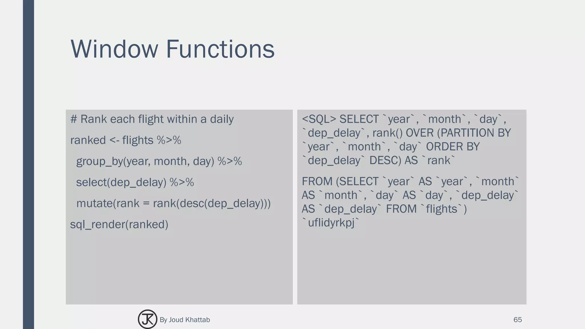
64. Window Functions
ranked # Source: lazy query [?? x 20]
# Database: spark_connection
year month day dep_delay rank
<int> <int> <int> <dbl> <int>
1 2013 1 5 327 1
2 2013 1 5 257 2
3 2013 1 5 225 3
4 2013 1 5 128 4
5 2013 1 5 127 5
6 2013 1 5 117 6
7 2013 1 5 111 7
8 2013 1 5 108 8
9 2013 1 5 105 9
10 2013 1 5 101 10
# ... with more rows
66By Joud Khattab

65. Performing Joins
■ It’s rare that a data analysis involves only a single table of data.
■ In practice, you’ll normally have many tables that contribute to an analysis, and you need
flexible tools to combine them.
■ In dplyr, there are three families of verbs that work with two tables at a time:
– Mutating joins, which add new variables to one table from matching rows in
another.
– Filtering joins, which filter observations from one table based on whether or not
they match an observation in the other table.
– Set operations, which combine the observations in the data sets as if they were set
elements.
■ All two-table verbs work similarly. The first two arguments are x and y, and provide the
tables to combine. The output is always a new table with the same type as x.
67By Joud Khattab

66. Performing Joins
The following statements are equivalent:
flights %>% left_join(airlines)
flights %>% left_join(airlines, by =
"carrier")
# Source: lazy query [?? x 20]
# Database: spark_connection
year month day dep_time sched_dep_time dep_delay arr_time
<int> <int> <int> <int> <int> <dbl> <int>
1 2013 1 1 517 515 2 830
2 2013 1 1 533 529 4 850
3 2013 1 1 542 540 2 923
4 2013 1 1 544 545 -1 1004
5 2013 1 1 554 600 -6 812
6 2013 1 1 554 558 -4 740
7 2013 1 1 555 600 -5 913
8 2013 1 1 557 600 -3 709
9 2013 1 1 557 600 -3 838
10 2013 1 1 558 600 -2 753
# ... with more rows
68By Joud Khattab

67. Sampling
■ You can use sample_n() and sample_frac() to take a random sample of rows:
– use sample_n() for a fixed number and sample_frac() for a fixed fraction.
■ Ex:
– sample_n(flights, 10)
– sample_frac(flights, 0.01)
69By Joud Khattab

68. SPARK SQL EXAMPLE
Analysis of babynames with dplyr
70By Joud Khattab

69. Analysis of babynames with dplyr
1. Setup.
2. Connect to Spark.
3. Total US births.
4. Aggregate data by name.
5. Most popular names (1986).
6. Most popular names (2014).
7. Shared names.
71By Joud Khattab

70. References
1. https://spark.apache.org/docs/latest/sql-programming-guide.html
2. http://spark.rstudio.com/
3. https://www.slideshare.net/databricks/spark-sql-deep-dive-melbroune
4. http://www.tutorialspoint.com/spark_sql/
5. https://www.youtube.com/watch?v=A7Ef_ZB884g
72By Joud Khattab

71. THANK YOU