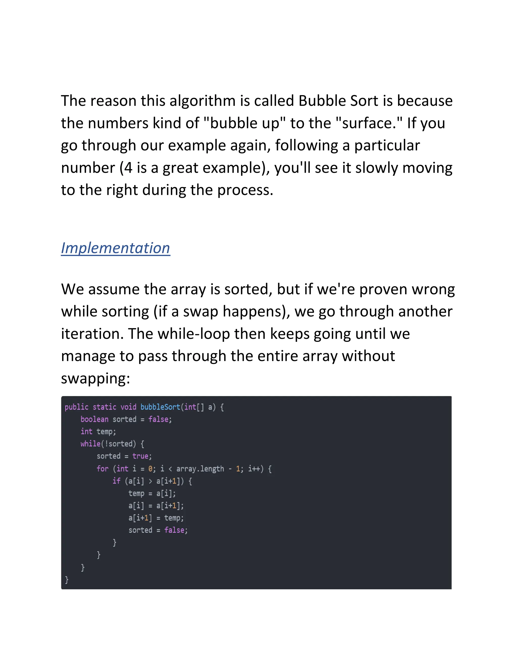
The document discusses various sorting algorithms in Java including bubble sort, insertion sort, selection sort, merge sort, heapsort, and quicksort. It provides explanations of how each algorithm works and comparisons of the time performance of each algorithm based on testing multiple runs. Quicksort and heapsort generally had the best performance while bubble sort consistently had the worst performance.

1. Sorting Algorithms in Java

2. Sorting data means arranging it in a certain order, often
in an array-like data structure. You can use various
ordering criteria, common ones being sorting numbers
from least to greatest or vice-versa, or sorting strings
lexicographically.
1. Bubble Sort :-
Explanation
Bubble sort works by swapping adjacent elements if
they're not in the desired order. This process repeats
from the beginning of the array until all elements are in
order.
We know that all elements are in order when we manage
to do the whole iteration without swapping at all - then
all elements we compared were in the desired order with
their adjacent elements, and by extension, the whole
array.

3. Here are the steps for sorting an array of numbers from
least to greatest:
• 4 2 1 5 3: The first two elements are in the wrong
order, so we swap them.
• 2 4 1 5 3: The second two elements are in the wrong
order too, so we swap.
• 2 1 4 5 3: These two are in the right order, 4 < 5, so
we leave them alone.
• 2 1 4 5 3: Another swap.
• 2 1 4 3 5: Here's the resulting array after one
iteration.
Because at least one swap occurred during the first pass
(there were actually three), we need to go through the
whole array again and repeat the same process.
By repeating this process, until no more swaps are made,
we'll have a sorted array.

4. The reason this algorithm is called Bubble Sort is because
the numbers kind of "bubble up" to the "surface." If you
go through our example again, following a particular
number (4 is a great example), you'll see it slowly moving
to the right during the process.
Implementation
We assume the array is sorted, but if we're proven wrong
while sorting (if a swap happens), we go through another
iteration. The while-loop then keeps going until we
manage to pass through the entire array without
swapping:

5. When using this algorithm, we have to be careful how we
state our swap condition.
For example, if I had used a[i] >= a[i+1] it could have
ended up with an infinite loop, because for equal
elements this relation would always be true, and hence
always swap them.
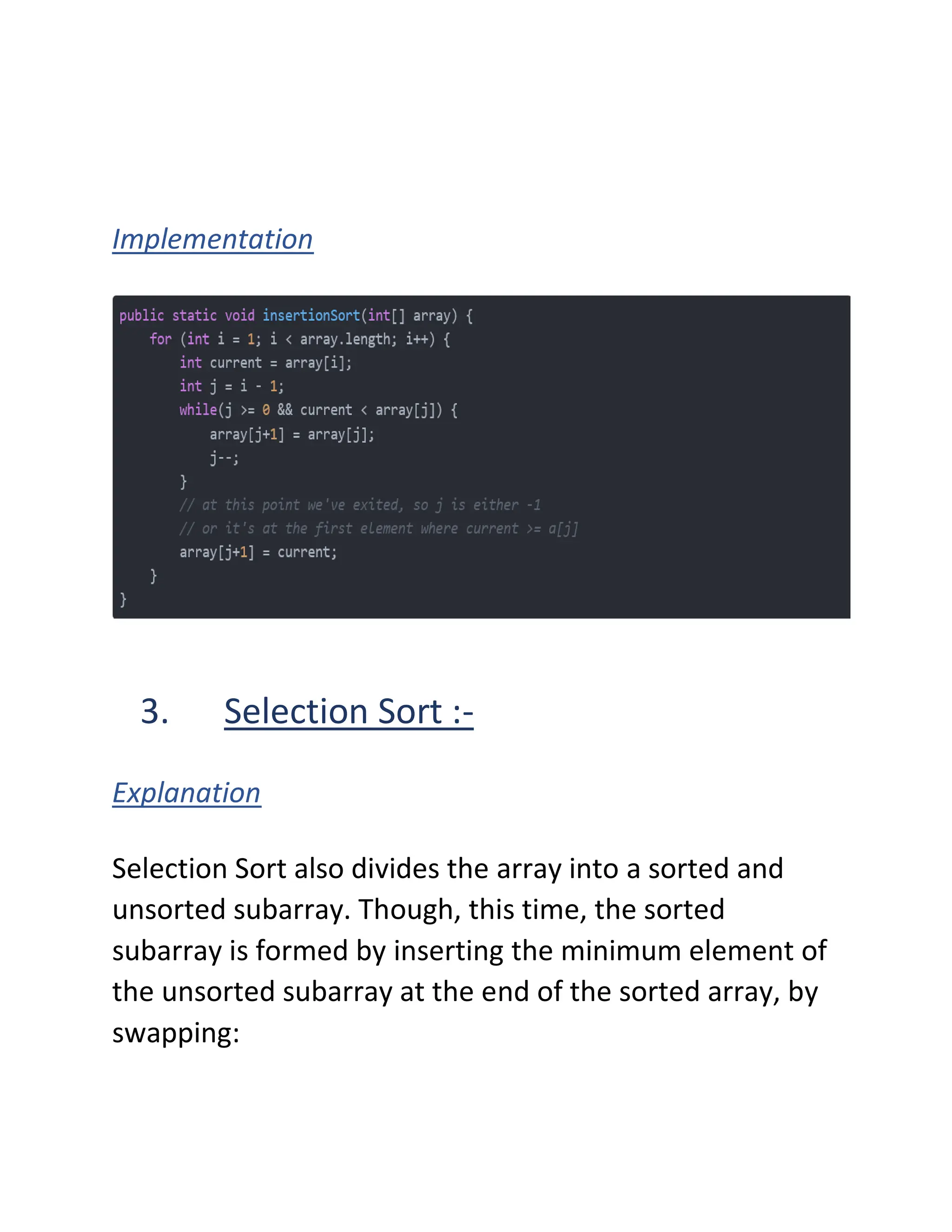
2. Insertion Sort :-
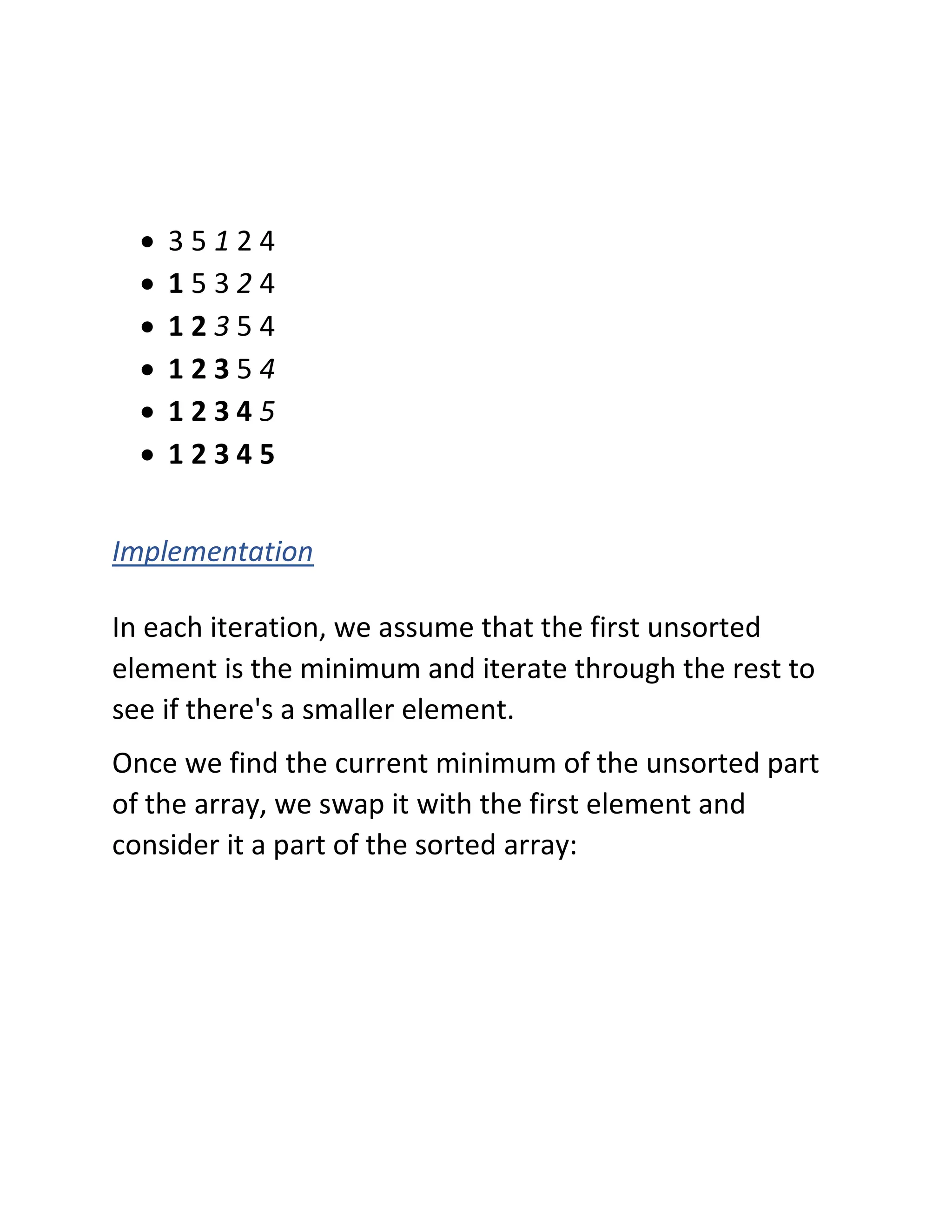
Explanation
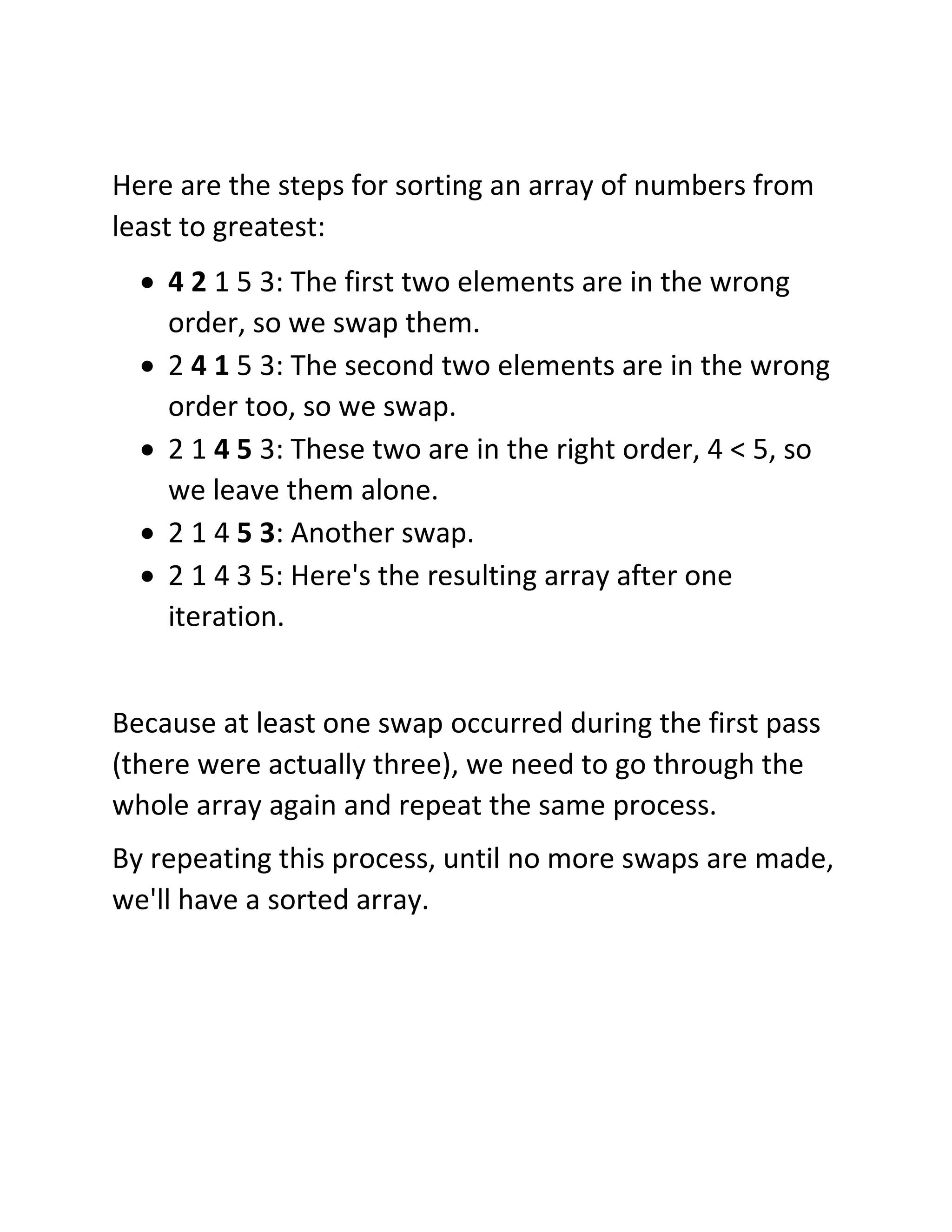
The idea behind Insertion Sort is dividing the array into
the sorted and unsorted subarrays.
The sorted part is of length 1 at the beginning and is
corresponding to the first (left-most) element in the
array. We iterate through the array and during each
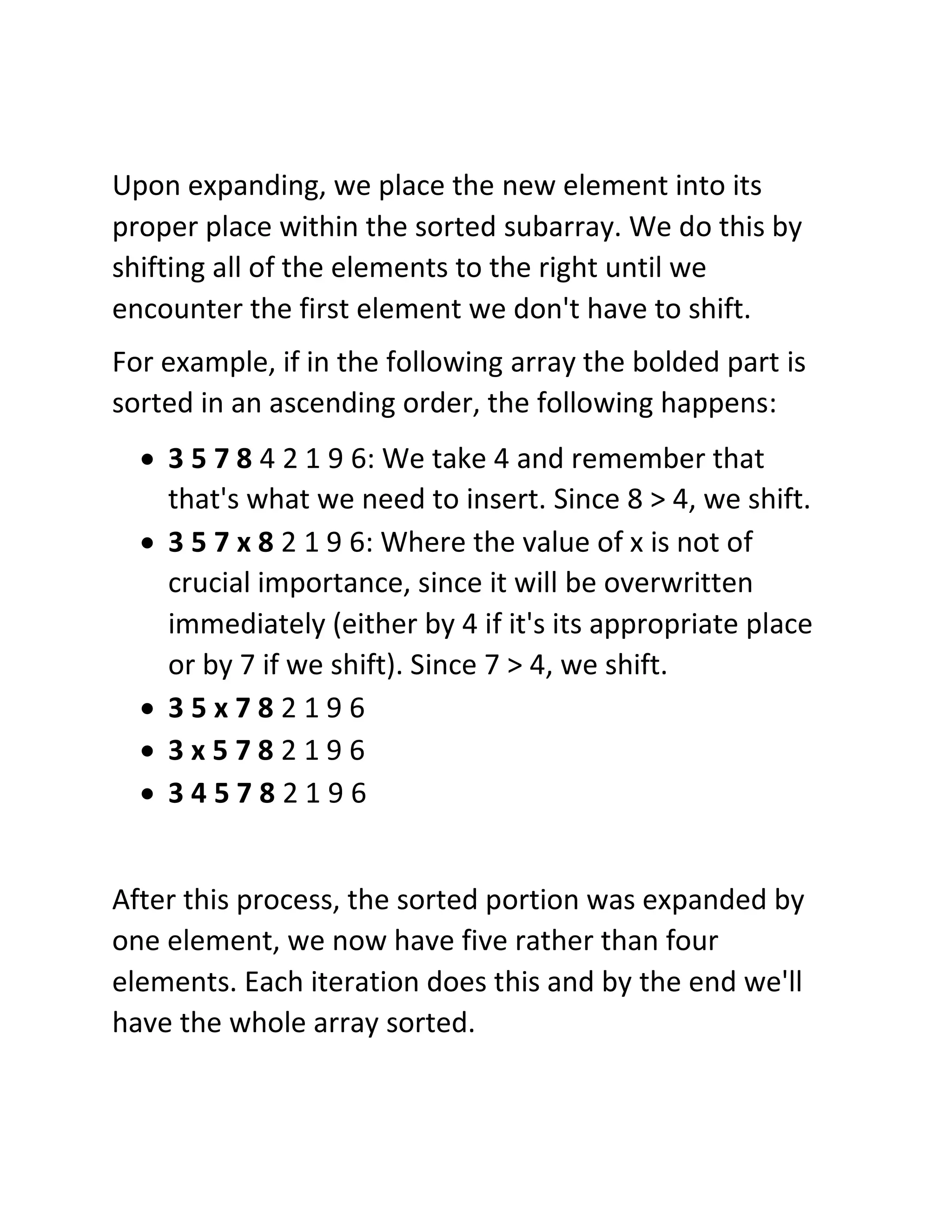
iteration, we expand the sorted portion of the array by
one element.

6. Upon expanding, we place the new element into its
proper place within the sorted subarray. We do this by
shifting all of the elements to the right until we
encounter the first element we don't have to shift.
For example, if in the following array the bolded part is
sorted in an ascending order, the following happens:
• 3 5 7 8 4 2 1 9 6: We take 4 and remember that
that's what we need to insert. Since 8 > 4, we shift.
• 3 5 7 x 8 2 1 9 6: Where the value of x is not of
crucial importance, since it will be overwritten
immediately (either by 4 if it's its appropriate place
or by 7 if we shift). Since 7 > 4, we shift.
• 3 5 x 7 8 2 1 9 6
• 3 x 5 7 8 2 1 9 6
• 3 4 5 7 8 2 1 9 6
After this process, the sorted portion was expanded by
one element, we now have five rather than four
elements. Each iteration does this and by the end we'll
have the whole array sorted.

7. Implementation
3. Selection Sort :-
Explanation
Selection Sort also divides the array into a sorted and
unsorted subarray. Though, this time, the sorted
subarray is formed by inserting the minimum element of
the unsorted subarray at the end of the sorted array, by
swapping:

8. • 3 5 1 2 4
• 1 5 3 2 4
• 1 2 3 5 4
• 1 2 3 5 4
• 1 2 3 4 5
• 1 2 3 4 5
Implementation
In each iteration, we assume that the first unsorted
element is the minimum and iterate through the rest to
see if there's a smaller element.
Once we find the current minimum of the unsorted part
of the array, we swap it with the first element and
consider it a part of the sorted array:

9. 4. Merge Sort :-
Explanation
Merge Sort uses recursion to solve the problem of
sorting more efficiently than algorithms previously
presented, and in particular it uses a divide and conquer
approach.
Using both of these concepts, we'll break the whole array
down into two subarrays and then:
1.Sort the left half of the array (recursively)
2.Sort the right half of the array (recursively)
3.Merge the solutions

10. This tree is meant to represent how the recursive calls
work. The arrays marked with the down arrow are the
ones we call the function for, while we're merging the
up-arrow ones going back up. So, you follow the down
arrow to the bottom of the tree, and then go back up and
merge.
In our example, we have the array 3 5 3 2 1, so we divide
it into 3 5 4 and 2 1. To sort them, we further divide them
into their components. Once we've reached the bottom,
we start merging up and sorting them as we go.

11. Implementation
The core function works pretty much as laid out in the
explanation. We're just passing indexes left and right
which are indexes of the left-most and right-most
element of the subarray we want to sort. Initially, these
should be 0 and array.length-1, depending on
implementation.
The base of our recursion ensures we exit when we've
finished, or when right and left meet each other. We find
a midpoint mid, and sort subarrays left and right of it
recursively, ultimately merging our solutions.
If you remember our tree graphic, you might wonder
why don't we create two new smaller arrays and pass
them on instead. This is because on really long arrays,
this would cause huge memory consumption for
something that's essentially unnecessary.
Merge Sort already doesn't work in-place because of the
merge step, and this would only serve to worsen its
memory efficiency. The logic of our tree of recursion
otherwise stays the same, though, we just have to follow
the indexes we're using:

12. To merge the sorted subarrays into one, we'll need to
calculate the length of each and make temporary arrays
to copy them into, so we could freely change our main
array.
After copying, we go through the resulting array and
assign it the current minimum. Because our subarrays
are sorted, we just chose the lesser of the two elements
that haven't been chosen so far, and move the iterator
for that subarray forward:

14. 5.Heapsort :-
Explanation
To properly understand why Heapsort works, you must
first understand the structure it's based on - the heap.
We'll be talking in terms of a binary heap specifically, but
you can generalize most of this to other heap structures
as well.
A heap is a tree that satisfies the heap property, which is
that for each node, all of its children are in a given
relation to it. Additionally, a heap must be almost
complete. An almost complete binary tree of depth d has
a subtree of depth d-1 with the same root that is
complete, and in which each node with a left descendent
has a complete left subtree. In other words, when adding
a node, we always go for the leftmost position in the
highest incomplete level.
If the heap is a max-heap, then all of the children are
smaller than the parent, and if it's a min-heap all of them
are larger.

15. In other words, as you move down the tree, you get to
smaller and smaller numbers (min-heap) or greater and
greater numbers (max-heap). Here's an example of a
max-heap:
We can represent this max-heap in memory as an array
in the following way:
8 5 6 3 1 2 4

16. You can envision it as reading from the graph level by
level, left to right. What we have achieved by this is that
if we take the kth element in the array, its children's
positions are 2*k+1 and 2*k+2 (assuming the indexing
starts at 0). You can check this for yourself.
Conversely, for the kth element the parent's position is
always (k-1)/2.
Knowing this, you can easily "max-heapify" any given
array. For each element, check if any of its children are
smaller than it. If they are, swap one of them with the
parent, and recursively repeat this step with the parent
(because the new large element might still be bigger than
its other child).
Leaves have no children, so they're trivially max-heaps of
their own:

17. • 6 1 8 3 5 2 4: Both children are smaller than the
parent, so everything stays the same.
• 6 1 8 3 5 2 4: Because 5 > 1, we swap them. We
recursively heapify for 5 now.
• 6 5 8 3 1 2 4: Both of the children are smaller, so
nothing happens.
• 6 5 8 3 1 2 4: Because 8 > 6, we swap them.
• 8 5 6 3 1 2 4: We got the heap pictured above!
Once we've learned to heapify an array the rest is pretty
simple. We swap the root of the heap with the end of the
array, and shorten the array by one.
We heapify the shortened array again, and repeat the
process:
• 8 5 6 3 1 2 4
• 4 5 6 3 1 2 8: swapped
• 6 5 4 3 1 2 8: heapified
• 2 5 4 3 1 6 8: swapped
• 5 2 4 2 1 6 8: heapified
• 1 2 4 2 5 6 8: swapped
And so on, I'm sure you can see the pattern emerging.

18. Implementation

19. 6.Quicksort :-
Explanation
Quicksort is another Divide and Conquer algorithm. It
picks one element of an array as the pivot and sorts all of
the other elements around it, for example smaller
elements to the left, and larger to the right.
This guarantees that the pivot is in its proper place after
the process. Then the algorithm recursively does the
same for the left and right portions of the array.
Implementation

20. Performance Comparison :-

21. time(ns)
Bubble
Sort
Insertion
Sort
Selection
Sort
MergeS
ort
HeapSort
QuickSor
t
First Run 266,089,476 21,973,989 66,603,076 5,511,069 5,283,411 4,156,005
Second
Run
323,692,591 29,138,068 80,963,267 8,075,023 6,420,768 7,060,203
Third Run 303,853,052 21,380,896 91,810,620 7,765,258 8,009,711 7,622,817
Fourth
Run
410,171,593 30,995,411 96,545,412 6,560,722 5,837,317 2,358,377
Fifth Run 315,602,328 26,119,110 95,742,699 5,471,260 14,629,836 3,331,834
Sixth Run 286,841,514 26,789,954 90,266,152 9,898,465 4,671,969 4,401,080
Seventh
Run
384,841,823 18,979,289 72,569,462 5,135,060 10,348,805 4,982,666
Eight Run 393,849,249 34,476,528 107,951,645 8,436,103 10,142,295
13,678,77
2
Ninth
Run
306,140,830 57,831,705 138,244,799 5,154,343 5,654,133 4,663,260
Tenth
Run
306,686,339 34,594,400 89,442,602 5,601,573 4,675,390 3,148,027
We can evidently see that Bubble Sort is the worst when it comes to performance. Avoid using
it in production if you can't guarantee that it'll handle only small collections and it won't stall
the application.
HeapSort and QuickSort are the best performance-wise. Although they're outputting similar
results, QuickSort tends to be a bit better and more consistent