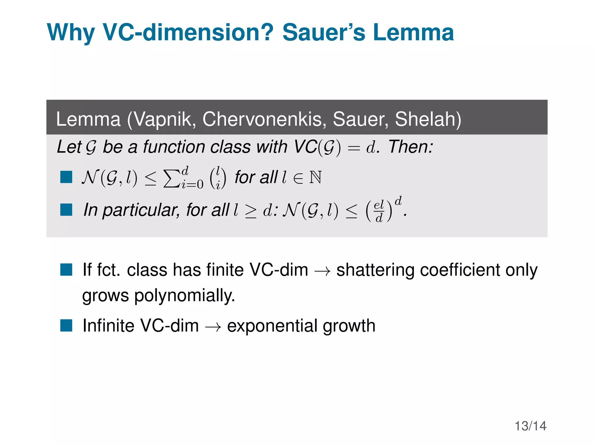
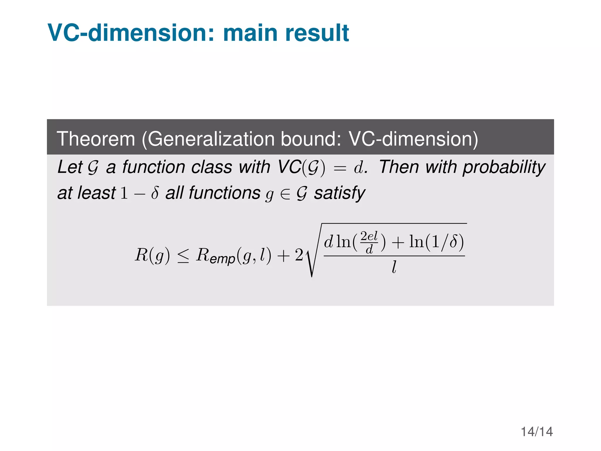
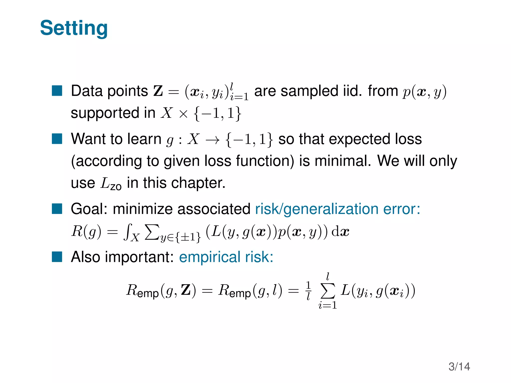
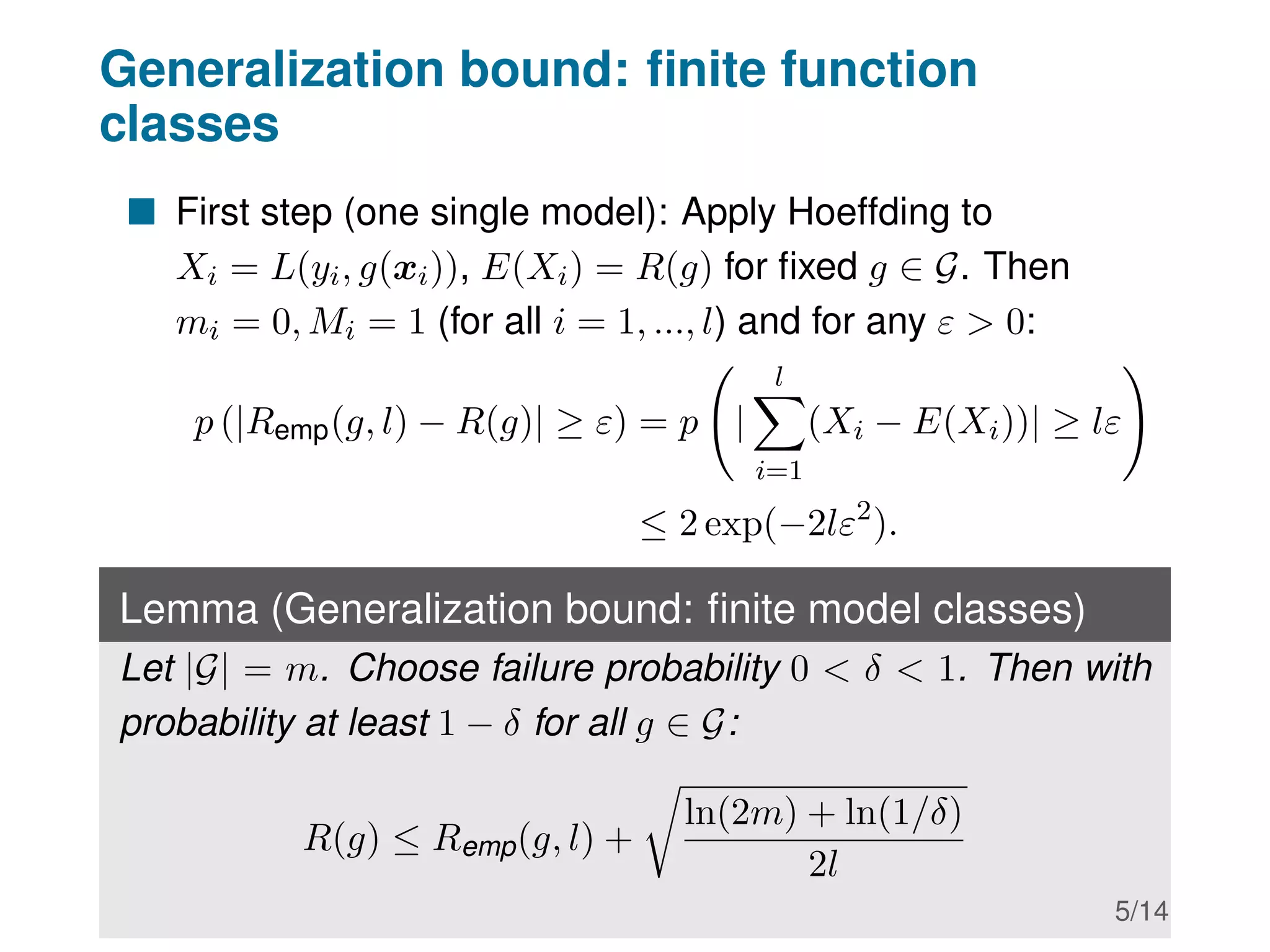
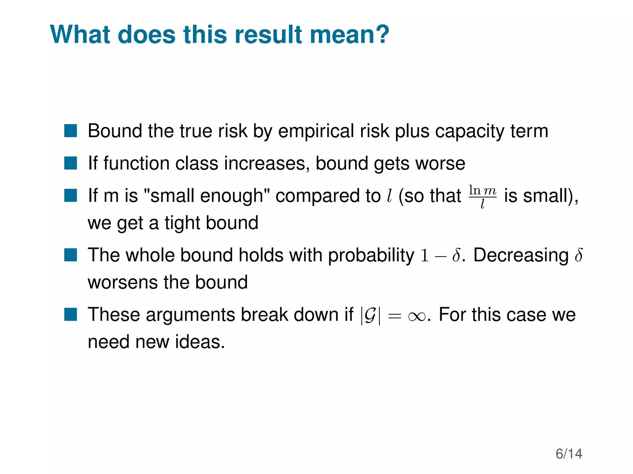
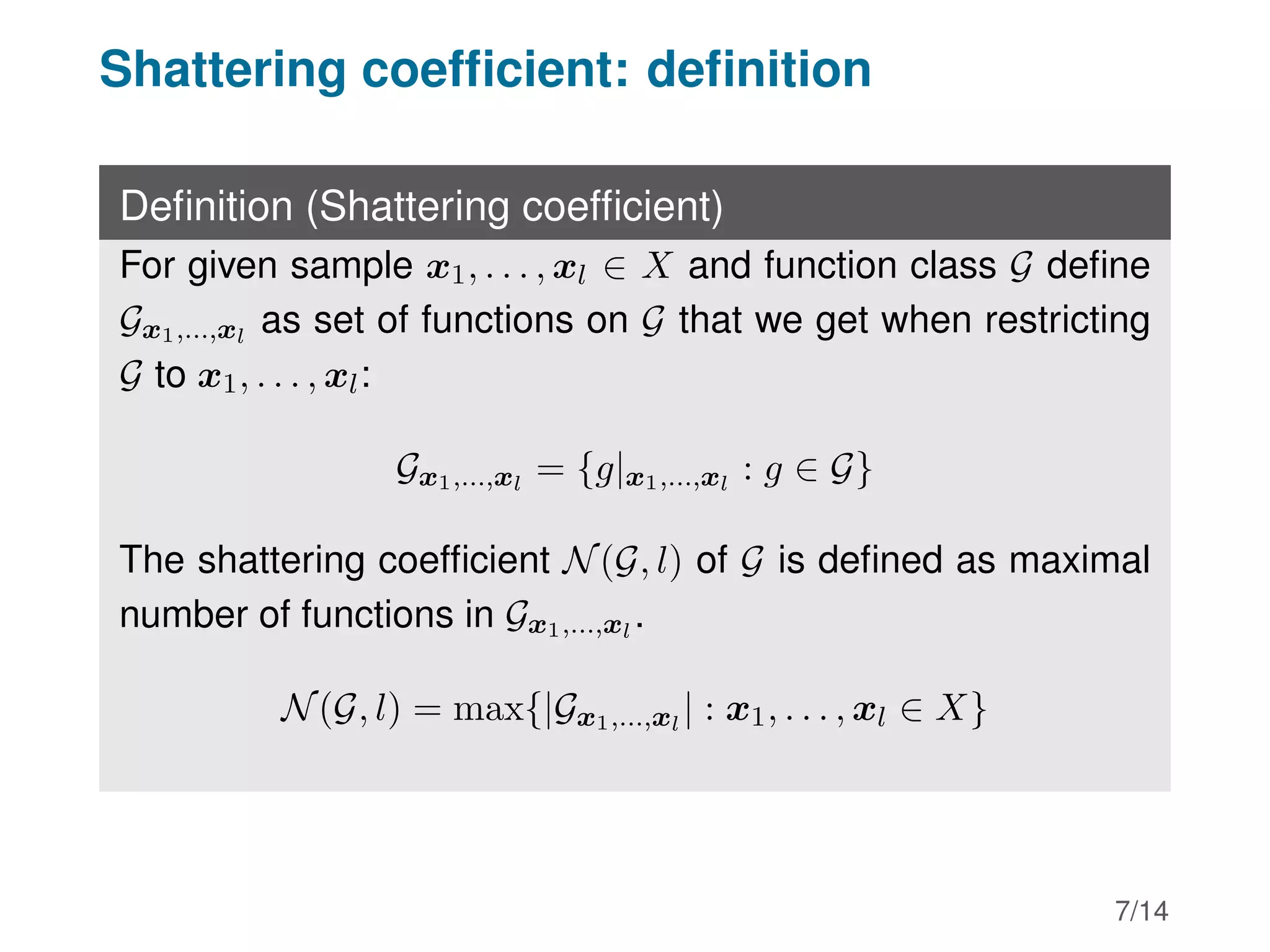
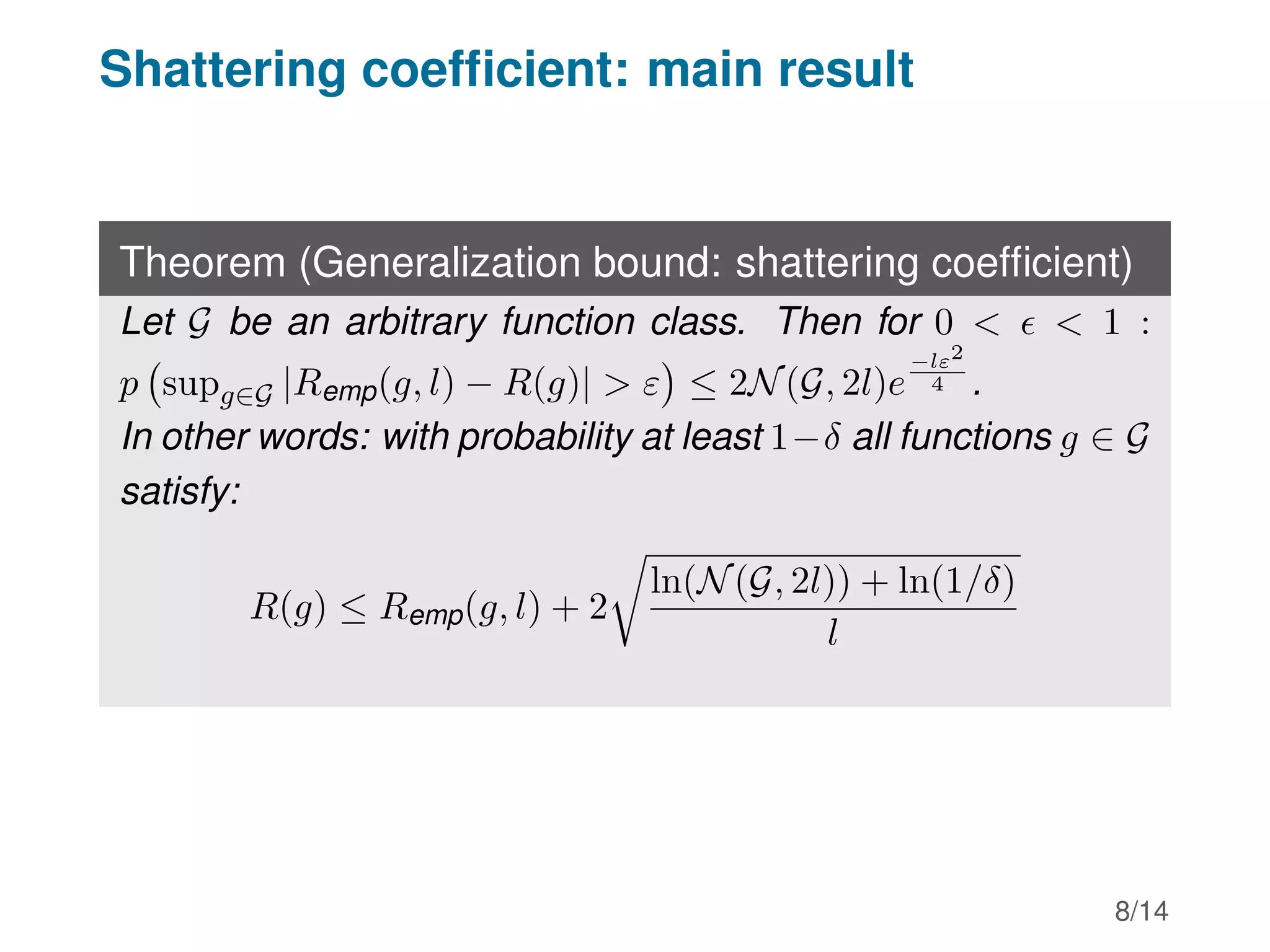
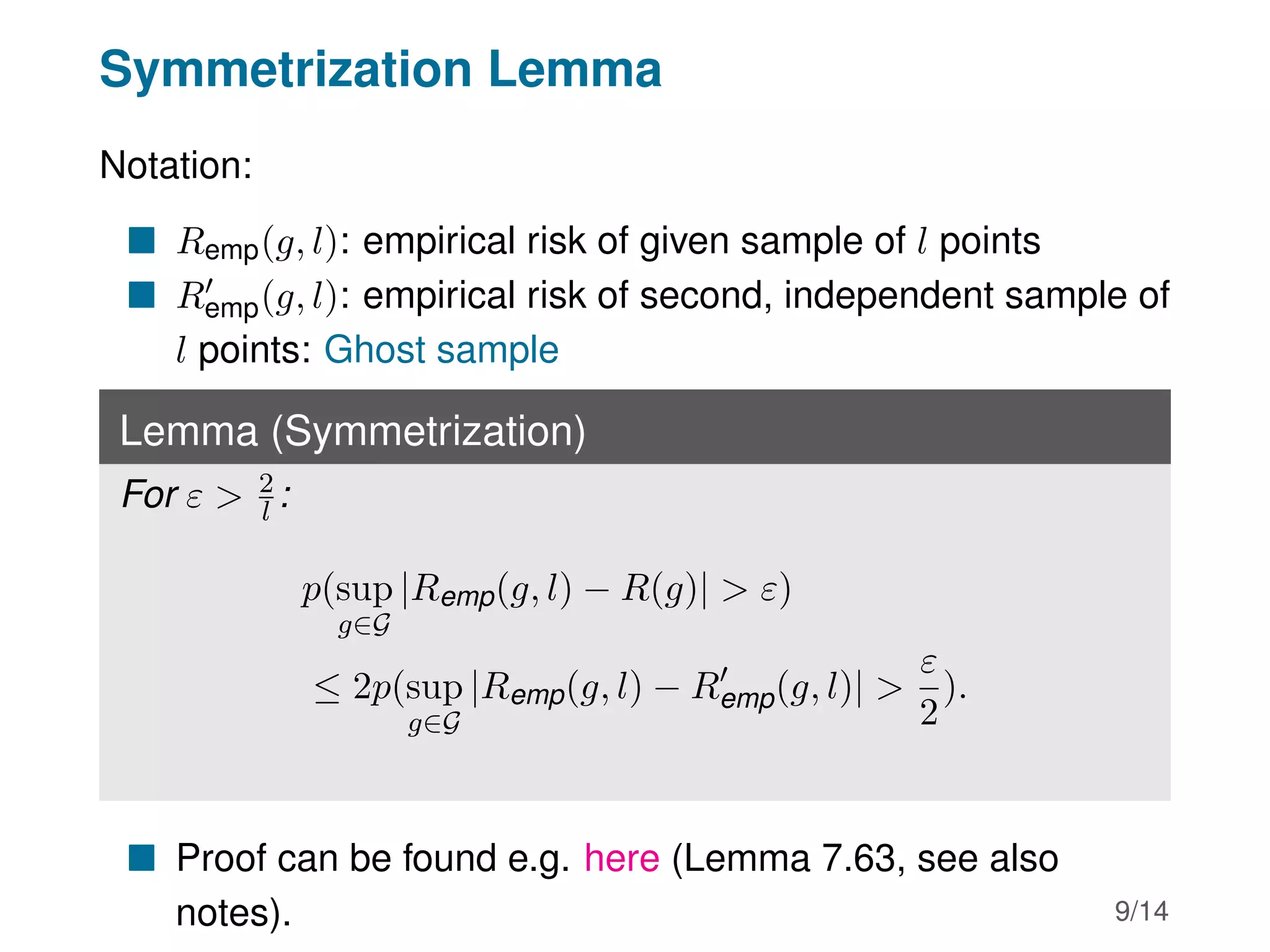
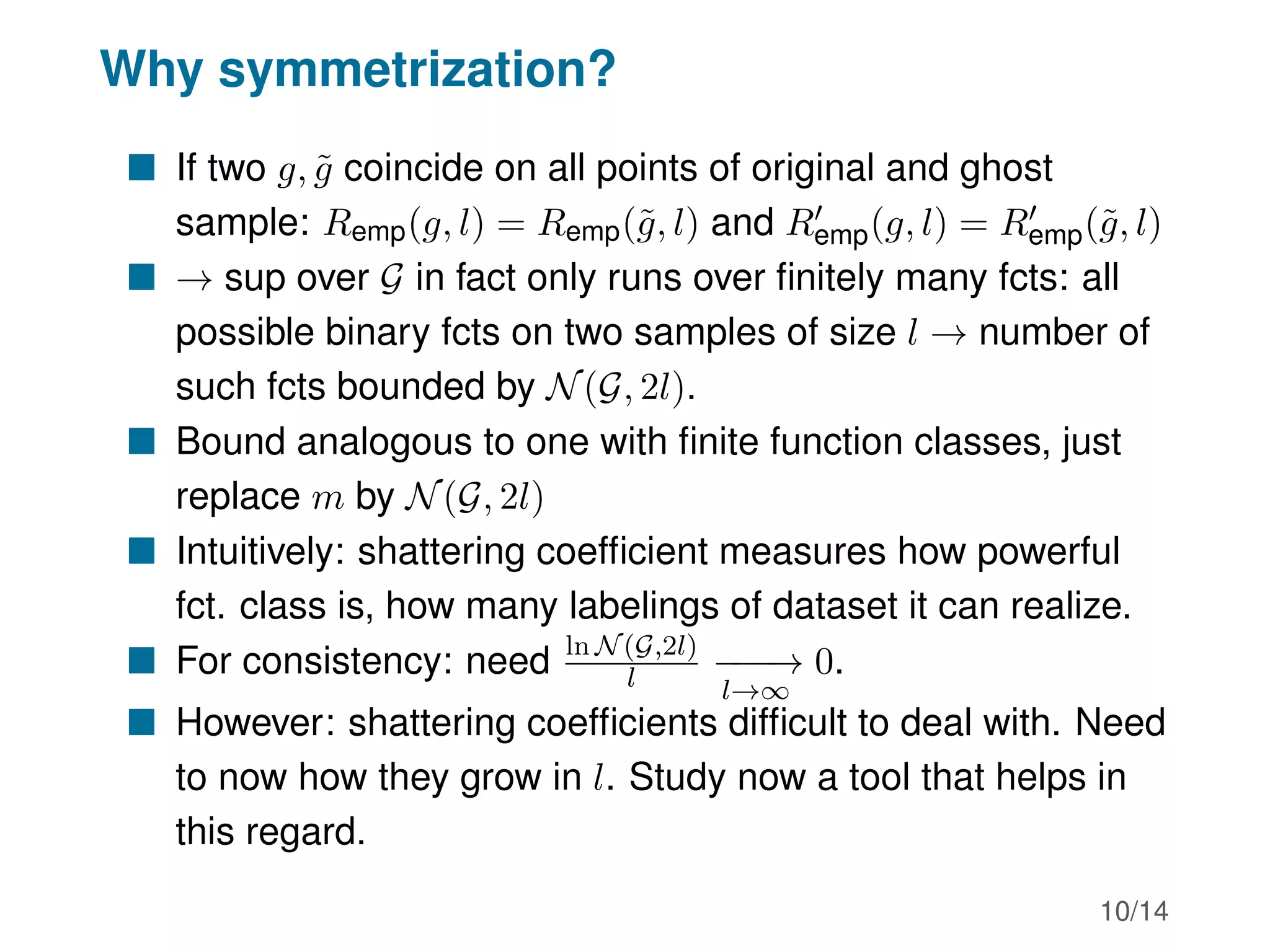
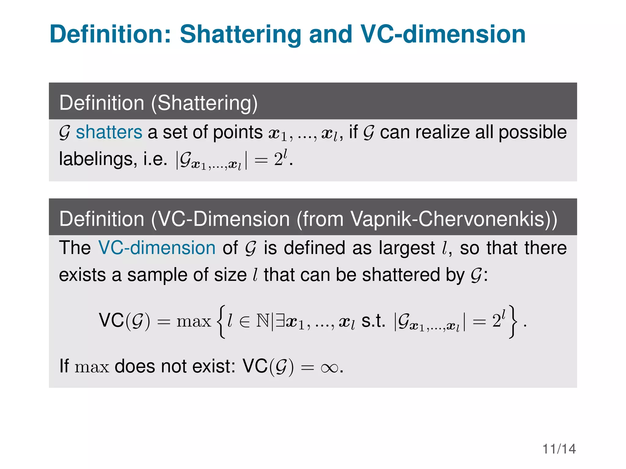
ASSIGNMENT 4:
VC DIMENSION
Institute for Machine Learning
Contact
Heads:
Markus Holzleitner,
Andreas Radler
————
Institute for Machine Learning
Johannes Kepler University
Altenberger Str. 69
A-4040 Linz
————
E-Mail: theoretical@ml.jku.at
Only mails to this list are answered!
Institute Homepage
1/14
Copyright statement:
This material, no matter whether in printed or electronic form,
may be used for personal and non-commercial educational use
only. Any reproduction of this material, no matter whether as a
whole or in parts, no matter whether in printed or in electronic
form, requires explicit prior acceptance of the authors.
2/14
Setting
 Data points Z = (xi, yi)l
i=1 are sampled iid. from p(x, y)
supported in X × {−1, 1}
 Want to learn g : X → {−1, 1} so that expected loss
(according to given loss function) is minimal. We will only
use Lzo in this chapter.
 Goal: minimize associated risk/generalization error:
R(g) =
R
X
P
y∈{±1} (L(y, g(x))p(x, y)) dx
 Also important: empirical risk:
Remp(g, Z) = Remp(g, l) = 1
l
l
P
i=1
L(yi, g(xi))
3/14
Hoeffding’s inequality
Lemma (Hoeffding)
Let X1, ..., Xl be independent random variables drawn accord-
ing to p. Assume further that Xi ∈ [mi, Mi]. Then for t ≥ 0:
p
l
X
i=1
(Xi − E(Xi)) ≥ t
!
≤ exp −
2t2
Pl
i=1(Mi − mi)2
!
4/14
Generalization bound: finite function
classes
 First step (one single model): Apply Hoeffding to
Xi = L(yi, g(xi)), E(Xi) = R(g) for fixed g ∈ G. Then
mi = 0, Mi = 1 (for all i = 1, ..., l) and for any ε  0:
p (|Remp(g, l) − R(g)| ≥ ε) = p |
l
X
i=1
(Xi − E(Xi))| ≥ lε
!
≤ 2 exp(−2lε2
).
Lemma (Generalization bound: finite model classes)
Let |G| = m. Choose failure probability 0  δ  1. Then with
probability at least 1 − δ for all g ∈ G:
R(g) ≤ Remp(g, l) +
r
ln(2m) + ln(1/δ)
2l
5/14
What does this result mean?
 Bound the true risk by empirical risk plus capacity term
 If function class increases, bound gets worse
 If m is small enough compared to l (so that ln m
l is small),
we get a tight bound
 The whole bound holds with probability 1 − δ. Decreasing δ
worsens the bound
 These arguments break down if |G| = ∞. For this case we
need new ideas.
6/14
Shattering coefficient: definition
Definition (Shattering coefficient)
For given sample x1, . . . , xl ∈ X and function class G define
Gx1,...,xl
as set of functions on G that we get when restricting
G to x1, . . . , xl:
Gx1,...,xl
= {g|x1,...,xl
: g ∈ G}
The shattering coefficient N(G, l) of G is defined as maximal
number of functions in Gx1,...,xl
.
N(G, l) = max{|Gx1,...,xl
| : x1, . . . , xl ∈ X}
7/14
Shattering coefficient: main result
Theorem (Generalization bound: shattering coefficient)
Let G be an arbitrary function class. Then for 0    1 :
p supg∈G |Remp(g, l) − R(g)|  ε

≤ 2N(G, 2l)e
−lε2
4 .
In other words: with probability at least 1−δ all functions g ∈ G
satisfy:
R(g) ≤ Remp(g, l) + 2
r
ln(N(G, 2l)) + ln(1/δ)
l
8/14
Symmetrization Lemma
Notation:
 Remp(g, l): empirical risk of given sample of l points
 R0
emp(g, l): empirical risk of second, independent sample of
l points: Ghost sample
Lemma (Symmetrization)
For ε  2
l :
p(sup
g∈G
|Remp(g, l) − R(g)|  ε)
≤ 2p(sup
g∈G
|Remp(g, l) − R0
emp(g, l)| 
ε
2
).
 Proof can be found e.g. here (Lemma 7.63, see also
notes). 9/14
Why symmetrization?
 If two g, g̃ coincide on all points of original and ghost
sample: Remp(g, l) = Remp(g̃, l) and R0
emp(g, l) = R0
emp(g̃, l)
 → sup over G in fact only runs over finitely many fcts: all
possible binary fcts on two samples of size l → number of
such fcts bounded by N(G, 2l).
 Bound analogous to one with finite function classes, just
replace m by N(G, 2l)
 Intuitively: shattering coefficient measures how powerful
fct. class is, how many labelings of dataset it can realize.
 For consistency: need ln N(G,2l)
l −
−
−
→
l→∞
0.
 However: shattering coefficients difficult to deal with. Need
to now how they grow in l. Study now a tool that helps in
this regard.
10/14
Definition: Shattering and VC-dimension
Definition (Shattering)
G shatters a set of points x1, ..., xl, if G can realize all possible
labelings, i.e. |Gx1,...,xl
| = 2l.
Definition (VC-Dimension (from Vapnik-Chervonenkis))
The VC-dimension of G is defined as largest l, so that there
exists a sample of size l that can be shattered by G:
VC(G) = max
n
l ∈ N|∃x1, ..., xl s.t. |Gx1,...,xl
| = 2l
o
.
If max does not exist: VC(G) = ∞.
11/14
VC-dimension: examples
 X = R, positive class=interior of closed interval, i.e.
G =

1[a,b] : a  b ∈ R .
 Positive class=interior of right triangles with sides adjacent
to right angle are parallel to aces. Right angle in lower left
corner. X = R2, G = {indicators of right triangles}.
 Positive class=interior of convex polygon, X = R2,
G = {indicators of convex polygons with d corners}
 X = R, G = {sgn (sin(tx)) : t ∈ R}. Then VC(G) = ∞
 X = Rr, G = {area above linear hyperplane}. Show in
exercises: VC(G) = r + 1
 X = Rr, ρ  0, G = {hyperplanes with margins at least γ}.
One can prove: if data are restricted to ball of radius R:
VC(G) = min

r, 2R2
γ2

+ 1.
12/14
Why VC-dimension? Sauer’s Lemma
Lemma (Vapnik, Chervonenkis, Sauer, Shelah)
Let G be a function class with VC(G) = d. Then:
 N(G, l) ≤
Pd
i=0
l
i

for all l ∈ N
 In particular, for all l ≥ d: N(G, l) ≤ el
d
d
.
 If fct. class has finite VC-dim → shattering coefficient only
grows polynomially.
 Infinite VC-dim → exponential growth
13/14
VC-dimension: main result
Theorem (Generalization bound: VC-dimension)
Let G a function class with VC(G) = d. Then with probability
at least 1 − δ all functions g ∈ G satisfy
R(g) ≤ Remp(g, l) + 2
s
d ln(2el
d ) + ln(1/δ)
l
14/14

Slides_A4.pdf

  • 1.
  • 2.
    Contact Heads: Markus Holzleitner, Andreas Radler ———— Institutefor Machine Learning Johannes Kepler University Altenberger Str. 69 A-4040 Linz ———— E-Mail: theoretical@ml.jku.at Only mails to this list are answered! Institute Homepage 1/14
  • 3.
    Copyright statement: This material,no matter whether in printed or electronic form, may be used for personal and non-commercial educational use only. Any reproduction of this material, no matter whether as a whole or in parts, no matter whether in printed or in electronic form, requires explicit prior acceptance of the authors. 2/14
  • 4.
    Setting Data pointsZ = (xi, yi)l i=1 are sampled iid. from p(x, y) supported in X × {−1, 1} Want to learn g : X → {−1, 1} so that expected loss (according to given loss function) is minimal. We will only use Lzo in this chapter. Goal: minimize associated risk/generalization error: R(g) = R X P y∈{±1} (L(y, g(x))p(x, y)) dx Also important: empirical risk: Remp(g, Z) = Remp(g, l) = 1 l l P i=1 L(yi, g(xi)) 3/14
  • 5.
    Hoeffding’s inequality Lemma (Hoeffding) LetX1, ..., Xl be independent random variables drawn accord- ing to p. Assume further that Xi ∈ [mi, Mi]. Then for t ≥ 0: p l X i=1 (Xi − E(Xi)) ≥ t ! ≤ exp − 2t2 Pl i=1(Mi − mi)2 ! 4/14
  • 6.
    Generalization bound: finitefunction classes First step (one single model): Apply Hoeffding to Xi = L(yi, g(xi)), E(Xi) = R(g) for fixed g ∈ G. Then mi = 0, Mi = 1 (for all i = 1, ..., l) and for any ε 0: p (|Remp(g, l) − R(g)| ≥ ε) = p | l X i=1 (Xi − E(Xi))| ≥ lε ! ≤ 2 exp(−2lε2 ). Lemma (Generalization bound: finite model classes) Let |G| = m. Choose failure probability 0 δ 1. Then with probability at least 1 − δ for all g ∈ G: R(g) ≤ Remp(g, l) + r ln(2m) + ln(1/δ) 2l 5/14
  • 7.
    What does thisresult mean? Bound the true risk by empirical risk plus capacity term If function class increases, bound gets worse If m is small enough compared to l (so that ln m l is small), we get a tight bound The whole bound holds with probability 1 − δ. Decreasing δ worsens the bound These arguments break down if |G| = ∞. For this case we need new ideas. 6/14
  • 8.
    Shattering coefficient: definition Definition(Shattering coefficient) For given sample x1, . . . , xl ∈ X and function class G define Gx1,...,xl as set of functions on G that we get when restricting G to x1, . . . , xl: Gx1,...,xl = {g|x1,...,xl : g ∈ G} The shattering coefficient N(G, l) of G is defined as maximal number of functions in Gx1,...,xl . N(G, l) = max{|Gx1,...,xl | : x1, . . . , xl ∈ X} 7/14
  • 9.
    Shattering coefficient: mainresult Theorem (Generalization bound: shattering coefficient) Let G be an arbitrary function class. Then for 0 1 : p supg∈G |Remp(g, l) − R(g)| ε ≤ 2N(G, 2l)e −lε2 4 . In other words: with probability at least 1−δ all functions g ∈ G satisfy: R(g) ≤ Remp(g, l) + 2 r ln(N(G, 2l)) + ln(1/δ) l 8/14
  • 10.
    Symmetrization Lemma Notation: Remp(g,l): empirical risk of given sample of l points R0 emp(g, l): empirical risk of second, independent sample of l points: Ghost sample Lemma (Symmetrization) For ε 2 l : p(sup g∈G |Remp(g, l) − R(g)| ε) ≤ 2p(sup g∈G |Remp(g, l) − R0 emp(g, l)| ε 2 ). Proof can be found e.g. here (Lemma 7.63, see also notes). 9/14
  • 11.
    Why symmetrization? Iftwo g, g̃ coincide on all points of original and ghost sample: Remp(g, l) = Remp(g̃, l) and R0 emp(g, l) = R0 emp(g̃, l) → sup over G in fact only runs over finitely many fcts: all possible binary fcts on two samples of size l → number of such fcts bounded by N(G, 2l). Bound analogous to one with finite function classes, just replace m by N(G, 2l) Intuitively: shattering coefficient measures how powerful fct. class is, how many labelings of dataset it can realize. For consistency: need ln N(G,2l) l − − − → l→∞ 0. However: shattering coefficients difficult to deal with. Need to now how they grow in l. Study now a tool that helps in this regard. 10/14
  • 12.
    Definition: Shattering andVC-dimension Definition (Shattering) G shatters a set of points x1, ..., xl, if G can realize all possible labelings, i.e. |Gx1,...,xl | = 2l. Definition (VC-Dimension (from Vapnik-Chervonenkis)) The VC-dimension of G is defined as largest l, so that there exists a sample of size l that can be shattered by G: VC(G) = max n l ∈ N|∃x1, ..., xl s.t. |Gx1,...,xl | = 2l o . If max does not exist: VC(G) = ∞. 11/14
  • 13.
    VC-dimension: examples X= R, positive class=interior of closed interval, i.e. G = 1[a,b] : a b ∈ R . Positive class=interior of right triangles with sides adjacent to right angle are parallel to aces. Right angle in lower left corner. X = R2, G = {indicators of right triangles}. Positive class=interior of convex polygon, X = R2, G = {indicators of convex polygons with d corners} X = R, G = {sgn (sin(tx)) : t ∈ R}. Then VC(G) = ∞ X = Rr, G = {area above linear hyperplane}. Show in exercises: VC(G) = r + 1 X = Rr, ρ 0, G = {hyperplanes with margins at least γ}. One can prove: if data are restricted to ball of radius R: VC(G) = min r, 2R2 γ2 + 1. 12/14
  • 14.
    Why VC-dimension? Sauer’sLemma Lemma (Vapnik, Chervonenkis, Sauer, Shelah) Let G be a function class with VC(G) = d. Then: N(G, l) ≤ Pd i=0 l i for all l ∈ N In particular, for all l ≥ d: N(G, l) ≤ el d d . If fct. class has finite VC-dim → shattering coefficient only grows polynomially. Infinite VC-dim → exponential growth 13/14
  • 15.
    VC-dimension: main result Theorem(Generalization bound: VC-dimension) Let G a function class with VC(G) = d. Then with probability at least 1 − δ all functions g ∈ G satisfy R(g) ≤ Remp(g, l) + 2 s d ln(2el d ) + ln(1/δ) l 14/14