Simple linear regression

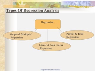
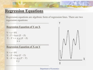
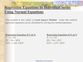
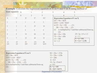
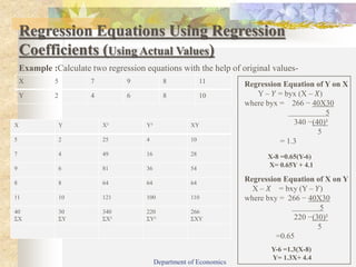
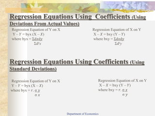
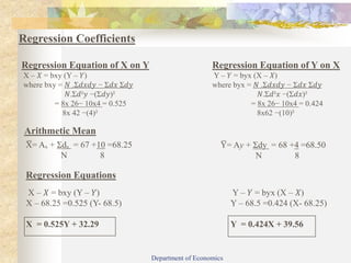
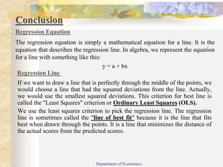
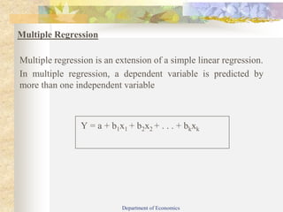
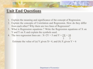
ECONOMICS
BASICSTATISTICS
Dr rekha choudhary
Department of Economics
Jai NarainVyas University,Jodhpur
Rajasthan

Introduction
The meaning of regression is “going back” or “returning”. The term
regression was first used in statistics by Sir Francis Galton a famous
scientist in 1877 in a study paper entitled, “ Regression towards Mediocrity
in Heredity Stature”
Wallin and Roberts have rightly said, “ It is often more important to find
out what the relation actually is, in order to estimate or predict one
variable (the dependent variable); and the statistical technique appropriate
to such a case is call regression analysis”
Regression analysis is very useful in economic and business world.

Objectives
After going through this unit, you will be able to:
 Understand the concept of Simple linear Regression;
 Define linear Regression , types of Regression, Regression coefficients
Merits and Demerits of Regression
Some particles problem of Regression in different series with different
methods.

Types Of Regression Analysis
Regression
Simple & Multiple
Regression
Linear & Non Linear
Regression
Partial & Total
Regression

Linear Regression
Definition
Generally, in two mutually related statistical series, the regression analysis is
based on graphic method. Under graphic method the values of X and Y
variables are plotted on a graph paper in the from of scatter diagram. When
two lines are drawn passing nearest to the dots, these are known as regression
lines. If these lines are straight, the regression is called as Linear
Simple Linear Regression
The study of linear regression between the values of X and Y variables is
called Simple linear regression. That variable, out of the two, which is
known is called independent variable, which is the base of prediction, and
that variable which is to be predicated is called dependent variable.

Regression
lines
Regression
Equations
Regression
coefficients
Simple Linear Regression

Regression Lines
Meaning
The regression line shows the average relationship between two variables. It
is also called Line of Best Fit.
If two variables X & Y are given, then there are two regression lines:
 Regression Line of X on Y
 Regression Line of Y on X
Nature of Regression Lines
 If r = ±1, then the two regression lines are coincident.
 If r = 0, then the two regression lines intersect each other at 90°.
 The nearer the regression lines are to each other, the greater will be the
degree of correlation.
 If regression lines rise from left to right upward, then correlation is
positive.

Functions of Regression Lines
1. The best Estimate
2. Degree and direction of
correlation
I. Positive
II. Negative
III. Perfect correlation one line
IV. Absence of correlation
V. Limited degree of correlation

Regression Equations
Regression equations are algebraic form of regression lines. There are two
regression equations:
Regression Equation of Y on X
Y = a + bX
Y – 𝑌 = 𝑏𝑦𝑥 (𝑋 − 𝑋)
Y – 𝑌 = 𝑟. σ 𝑦 (𝑋 − 𝑋)
σ 𝑥
Regression Equation of X on Y
X = a + bY
X – 𝑋 = 𝑏𝑥𝑦 (𝑌 − 𝑌)
X – 𝑋 = 𝑟. σ 𝑥 (𝑌 − 𝑌)
σ 𝑦

• Regression coefficient measures the average change in the
value of one variable for a unit change in the value of
another variable.
• These represent the slope of regression line
• There are two regression coefficients:
Regression Coefficients
Regression coefficient of Y on X:
byx = 𝑟. σ 𝑦
σ 𝑥
Regression coefficient of X on Y:
bxy = 𝑟. σ 𝑥
σ 𝑦

• Coefficient of correlation is the geometric mean of the regression
coefficients. i.e. r = √𝑏 𝑥𝑦 . 𝑏𝑦𝑥
• Both the regression coefficients must have the same algebraic sign.
• Coefficient of correlation must have the same sign as that of the
regression coefficients.
• Both the regression coefficients cannot be greater than unity.
• Regression coefficient is independent of change of origin but not of scale
Properties Of Regression Coefficients

Difference Between Correlation & Regression
Degree & Nature of Relationship
 Correlation is a measure of degree of relationship between X & Y
 Regression studies the nature of relationship between the variables so that one
may be able to predict the value of one variable on the basis of another.
Cause & Effect Relationship
 Correlation does not always assume cause and effect relationship between two
variables.
 Regression clearly expresses the cause and effect relationship between two
variables. The independent variable is the cause and dependent variable is effect.
Independent and Dependent Relationship
 In correlation analysis, there is no importance of independent and dependent
variables.
 In case of regression, there are two coefficients.
Non- sense Correlation
 Sometimes may be non-sense correlation between X and Y series, but regression
is never non-sense.

This method is also called as Least Square Method. Under this method,
regression equations can be calculated by solving two normal equations:
Regression Equations In Individual Series
Using Normal Equations
Y = a + bX
ƩY = Na + bƩX
ƩXY = a ƩX +bƩX²
X = a + bY
ƩX = Na + bƩY
ƩXY = a ƩY +bƩY²

Example: Calculate the regression equation of X on Y and Y on X using method of
least squares: X 1 2 3 4 5
Y 2 5 3 8 7
X Y X² Y² XY
1 2 1 4 2
2 5 4 25 10
3 3 9 9 9
4 8 16 64 32
5 7 25 49 35
15
ƩX
25
ƩY
55
ƩX²
151
ƩY²
88
ƩXY
ƩX = Na + bƩY
ƩXY = a ƩY +bƩY²
or 15 = 5a + 25b ……(1)
88 = 25a + 151b …..(2)
(i) is multiplied by 5 and then subtracted from eq.
(ii)
ƩY = Na + bƩX
ƩXY = a ƩX +bƩX²
or 25 = 5a + 15b ……(1)
88 = 15a + 55b …..(2)
(i) is multiplied by 3 and then subtracted from eq.
(ii)
88 = 15a + 55b
75 = 15a + 45b
13 = 10b
b = 1.3
25= 5a +15 x 1.3
a = 1.1
Y = a + bX
Y = 1.1 + 1.3X
88 = 25a + 151b
75 = 25a + 125b
13 = 26b
b = 0.5
15= 5a +25x0.5
a = 0.5
X = a + bY
X = 0.5 + 0.5 Y

Y – 𝑌 = byx (X – 𝑋)
where byx = 266 − 40X30
5
340 −(40)²
5
= 1.3
X – 𝑋 = bxy (Y – 𝑌)
where bxy = 266 − 40X30
5
220 −(30)²
5
=0.65
Regression Equations Using Regression
Coefficients (Using Actual Values)
Example :Calculate two regression equations with the help of original values-
X 5 7 9 8 11
Y 2 4 6 8 10
X Y X² Y² XY
5 2 25 4 10
7 4 49 16 28
9 6 81 36 54
8 8 64 64 64
11 10 121 100 110
40
ƩX
30
ƩY
340
ƩX²
220
ƩY²
266
ƩXY
X-8 =0.65(Y-6)
X= 0.65Y + 4.1
Y-6 =1.3(X-8)
Y= 1.3X+ 4.4

Y – 𝑌 = byx (X – 𝑋)
where byx = Σd𝑥d𝑦
Σd²x
Regression Equations Using Coefficients (Using
Deviations From Actual Values)
Y – 𝑌 = byx (X – 𝑋)
where byx = 𝑟. σ 𝑦
σ 𝑥
X – 𝑋 = bxy (Y – 𝑌)
where bxy = Σd𝑥d𝑦
Σd²y
Standard Deviations)
X – 𝑋 = bxy (Y – 𝑌)
where bxy = 𝑟. σ 𝑥
σ 𝑦

Deviations From Assumed Mean)
Height of Father 65 66 67 67 68 69 71 73
Height of Sons 67 68 64 68 72 70 69 70
Example: Calculate regression equations by calculating both regression coefficients by
assumed mean method
Height of Father X Height of Son Y Product of dₓ & dy
H in inches Deviation from
67
Square of
Deviation
H in inches Deviation
from 68
Square of
Deviation
X dₓ d²ₓ Y dy d²y dₓdy
65 -2 4 67 -1 1 2
66 -1 1 68 0 0 0
67 0 0 64 -4 16 0
67 0 0 68 0 0 0
68 1 1 72 4 16 4
69 2 4 70 2 4 4
71 4 16 69 1 1 4
73 6 36 70 2 4 12
N= 8 Σ𝑑𝑥 =10 Σ𝑑²𝑥 =62 Σ𝑑𝑦 =4 Σ𝑑²y =42 Σ𝑑𝑥𝑑𝑦=26

X – 𝑋 = bxy (Y – 𝑌)
where bxy = 𝑁 .Σ𝑑𝑥𝑑𝑦 − Σ𝑑𝑥 Σ𝑑𝑦
𝑁.Σ𝑑²𝑦 −(Σ𝑑𝑦)²
= 8x 26− 10x4 = 0.525
8x 42 −(4)²
Regression Coefficients
Y – 𝑌 = byx (X – 𝑋)
where byx = 𝑁 .Σ𝑑𝑥𝑑𝑦 − Σ𝑑𝑥 Σ𝑑𝑦
𝑁.Σ𝑑²𝑥 −(Σ𝑑𝑥)²
= 8x 26− 10x4 = 0.424
8x62 −(10)²
Arithmetic Mean
X̅ = Aₓ + Ʃdₓ = 67 +10 =68.25
N 8
Y̅ = Ay + Ʃdy = 68 +4 =68.50
N 8
Regression Equations
X – 𝑋 = bxy (Y – 𝑌)
X – 68.25 =0.525 (Y- 68.5)
X = 0.525Y + 32.29
Y – 𝑌 = byx (X – 𝑋)
Y – 68.5 =0.424 (X- 68.25)
Y = 0.424X + 39.56

The regression equation is simply a mathematical equation for a line. It is the
equation that describes the regression line. In algebra, we represent the equation
for a line with something like this:
y = a + bx
If we want to draw a line that is perfectly through the middle of the points, we
would choose a line that had the squared deviations from the line. Actually,
we would use the smallest squared deviations. This criterion for best line is
called the "Least Squares" criterion or Ordinary Least Squares (OLS).
We use the least squares criterion to pick the regression line. The regression
line is sometimes called the "line of best fit" because it is the line that fits
best when drawn through the points. It is a line that minimizes the distance of
the actual scores from the predicted scores.
Regression Line
Conclusion
Regression Equation

Multiple Regression
Multiple regression is an extension of a simple linear regression.
In multiple regression, a dependent variable is predicted by
more than one independent variable
Y = a + b1x1 + b2x2 + . . . + bkxk

Unit End Questions
1. Explain the meaning and significance of the concept of Regression.
2. Explain the concepts of Correlation and Regression. How do they differ
from each other? Why there are two lines of Regression?
3. What is Regression equations ? Write the Regression equations of X on
Y and Y on X and explain the symbols used.
4. The two regression lines are : X=2Y + 5 and Y = 2X + 10
3 3
Estimate the value of (a) Y given X= 4, and (b) X given Y = 6

Required Readings
B.L.Aggrawal (2009). Basic Statistics. New Age International Publisher, Delhi.
Gupta, S.C.(1990) Fundamentals of Statistics. Himalaya Publishing House, Mumbai
Elhance, D.N: Fundamental of Statistics
Singhal, M.L: Elements of Statistics
Nagar, A.L. and Das, R.K.: Basic Statistics
Croxton Cowden: Applied General Statistics
Nagar, K.N.: Sankhyiki ke mool tatva
Gupta, BN : Sankhyiki
https://www.bmj.com/about-bmj/resources-readers/publications/statistics-square-
one/11-correlation-and-regression

THANKS………

Simple linear regression

More Related Content

What's hot

Similar to Simple linear regression

More from RekhaChoudhary24

Recently uploaded

Simple linear regression