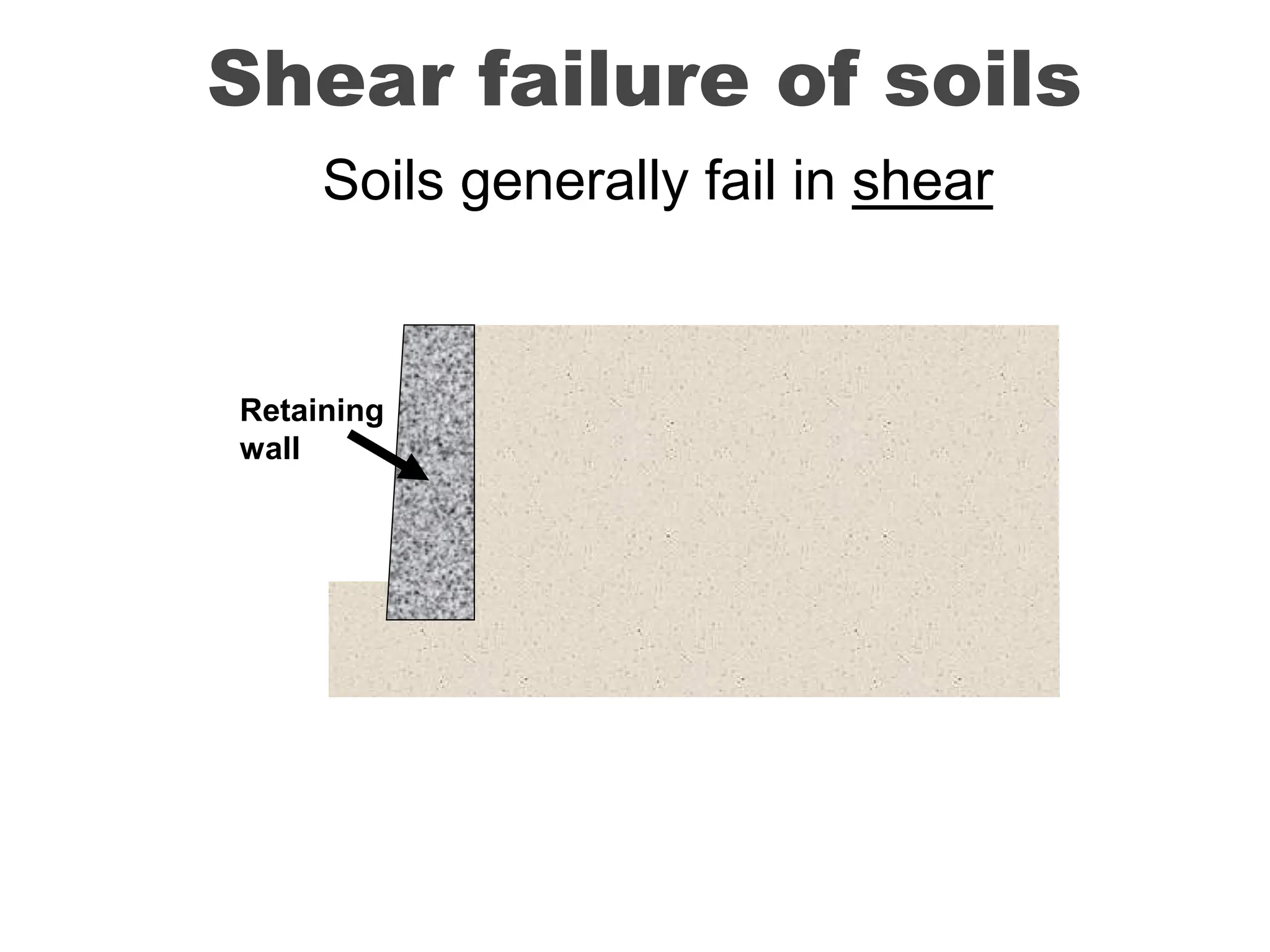
Retaining
wall
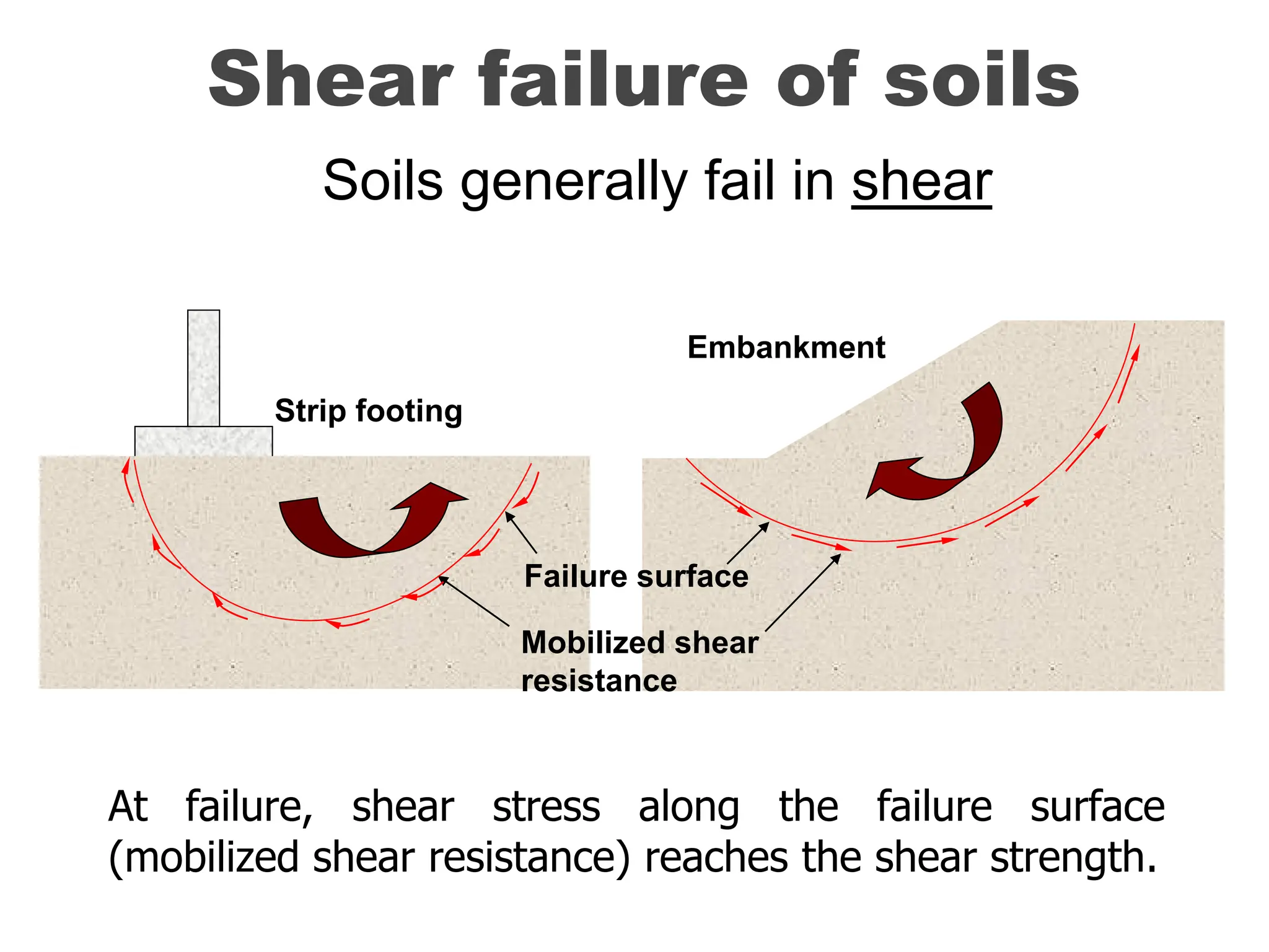
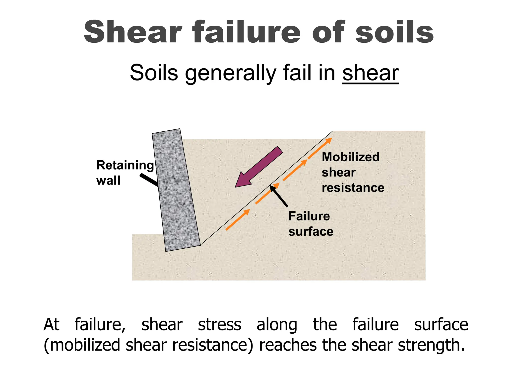
Shear failure ofsoils
At failure, shear stress along the failure surface
(mobilized shear resistance) reaches the shear strength.
Failure
surface
Mobilized
shear
resistance
Soils generally fail in shear
6.
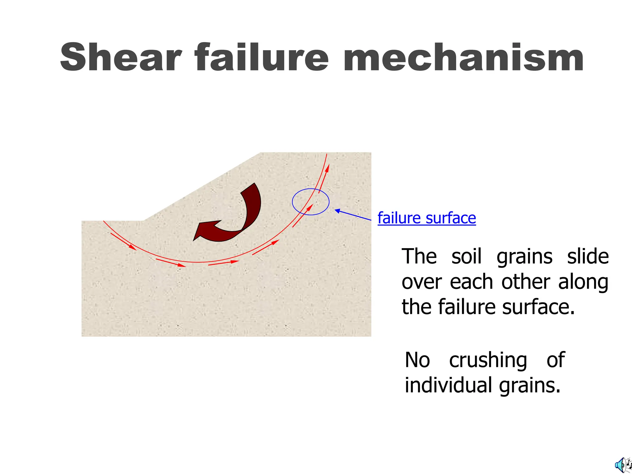
Shear failure mechanism
Thesoil grains slide
over each other along
the failure surface.
No crushing of
individual grains.
failure surface
7.
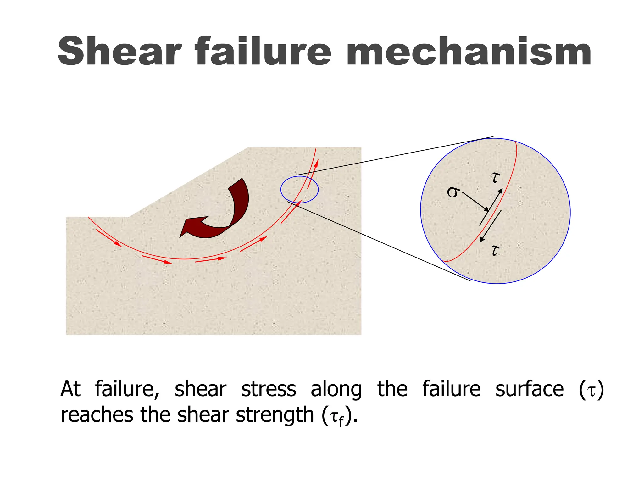
Shear failure mechanism
Atfailure, shear stress along the failure surface ()
reaches the shear strength (f).
8.
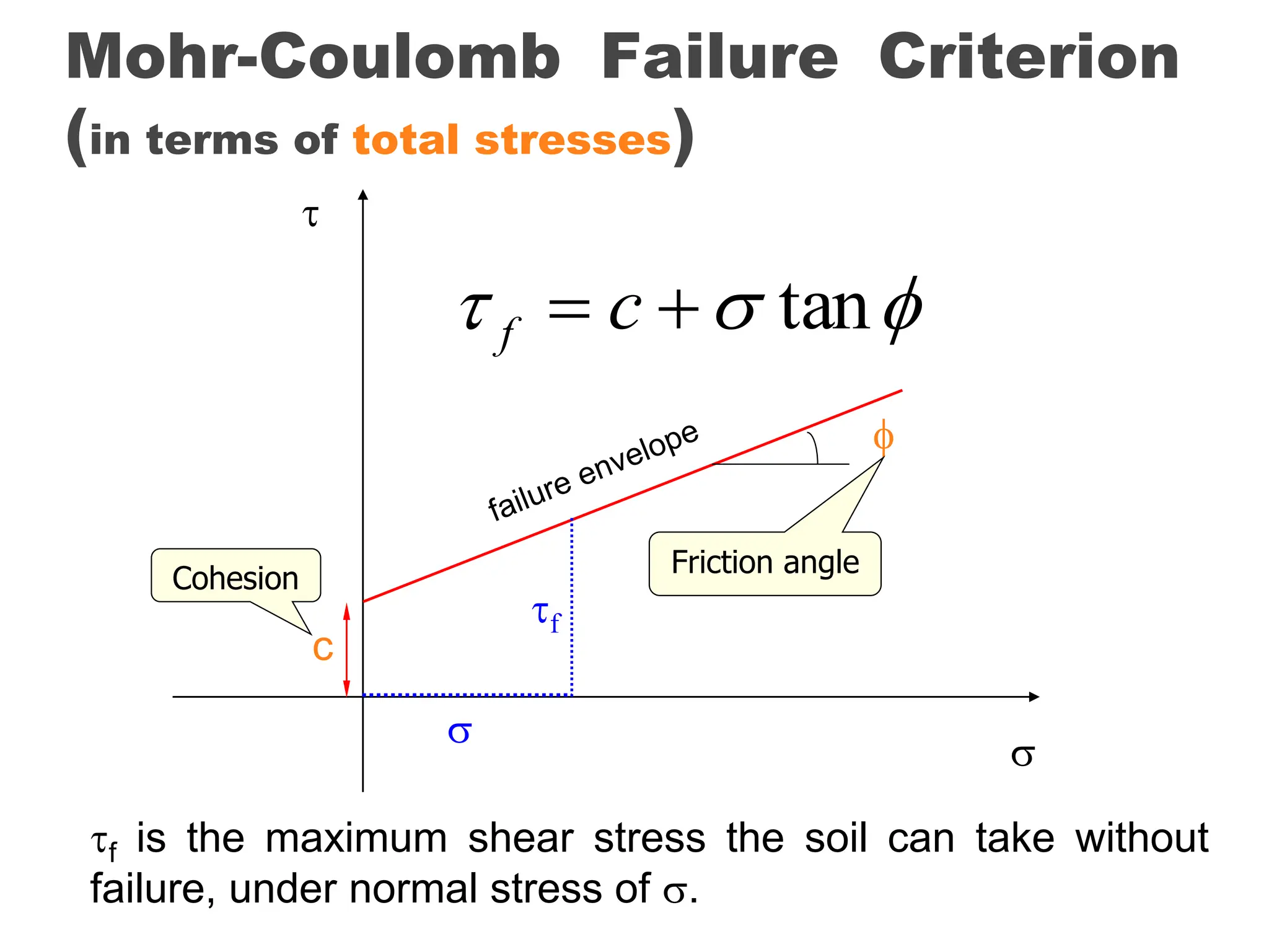
Mohr-Coulomb Failure Criterion
(interms of total stresses)
f is the maximum shear stress the soil can take without
failure, under normal stress of .
tan
c
f
c
Cohesion
Friction angle
f
9.
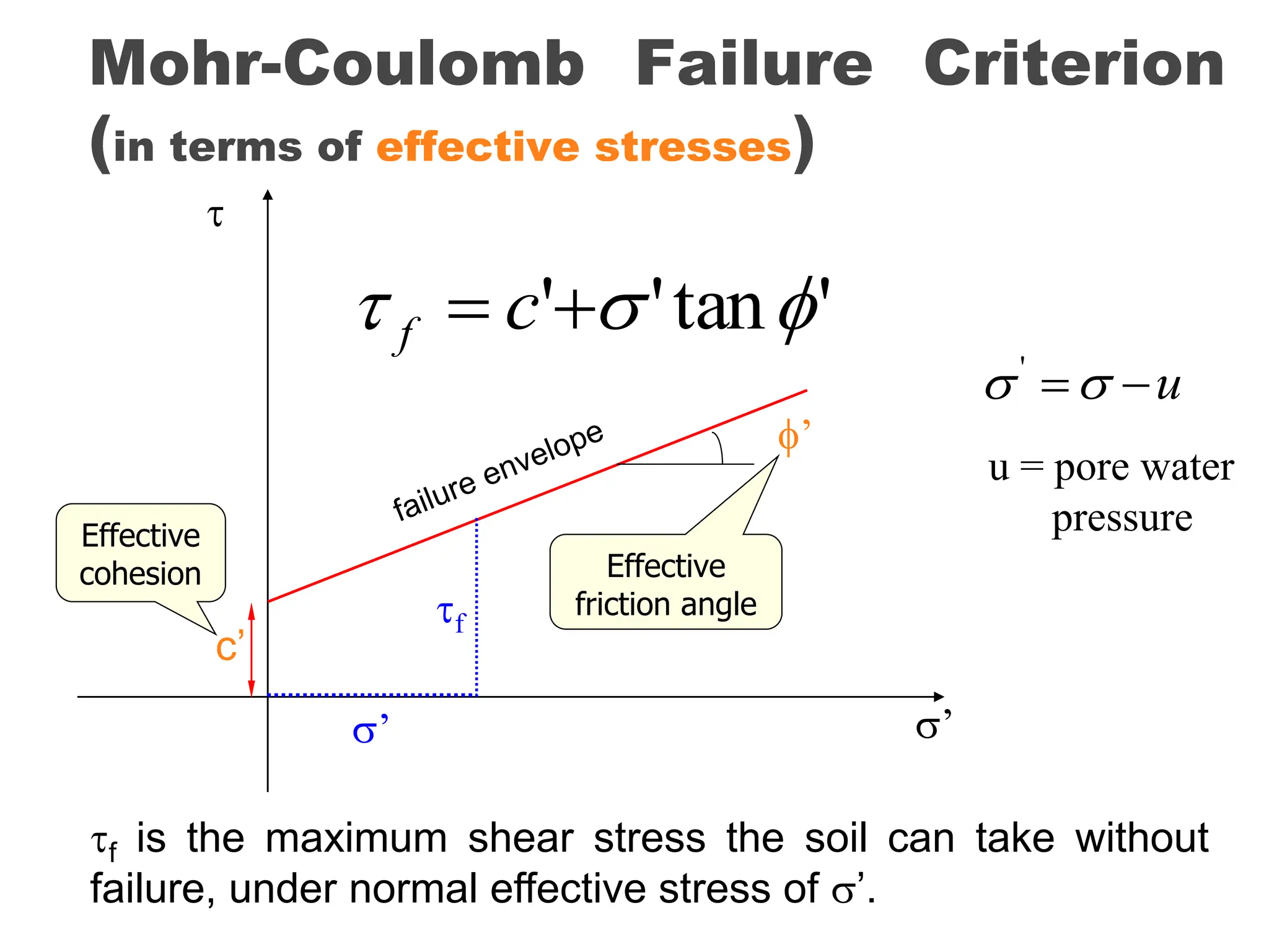
Mohr-Coulomb Failure Criterion
(interms of effective stresses)
f is the maximum shear stress the soil can take without
failure, under normal effective stress of ’.
’
'
tan
'
'
c
f
c’
’
Effective
cohesion Effective
friction angle
f
’
u
'
u = pore water
pressure
10.
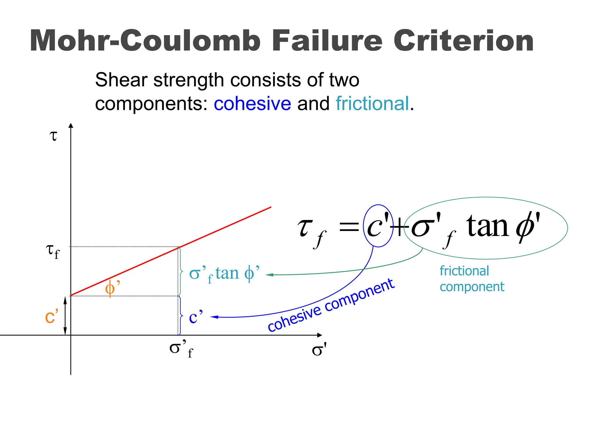
Mohr-Coulomb Failure Criterion
'
tan
'
'
f
f c
Shear strength consists of two
components: cohesive and frictional.
’f
f
’
'
c’ c’
’f tan ’ frictional
component
11.
c and are measures of shear strength.
Higher the values, higher the shear strength.
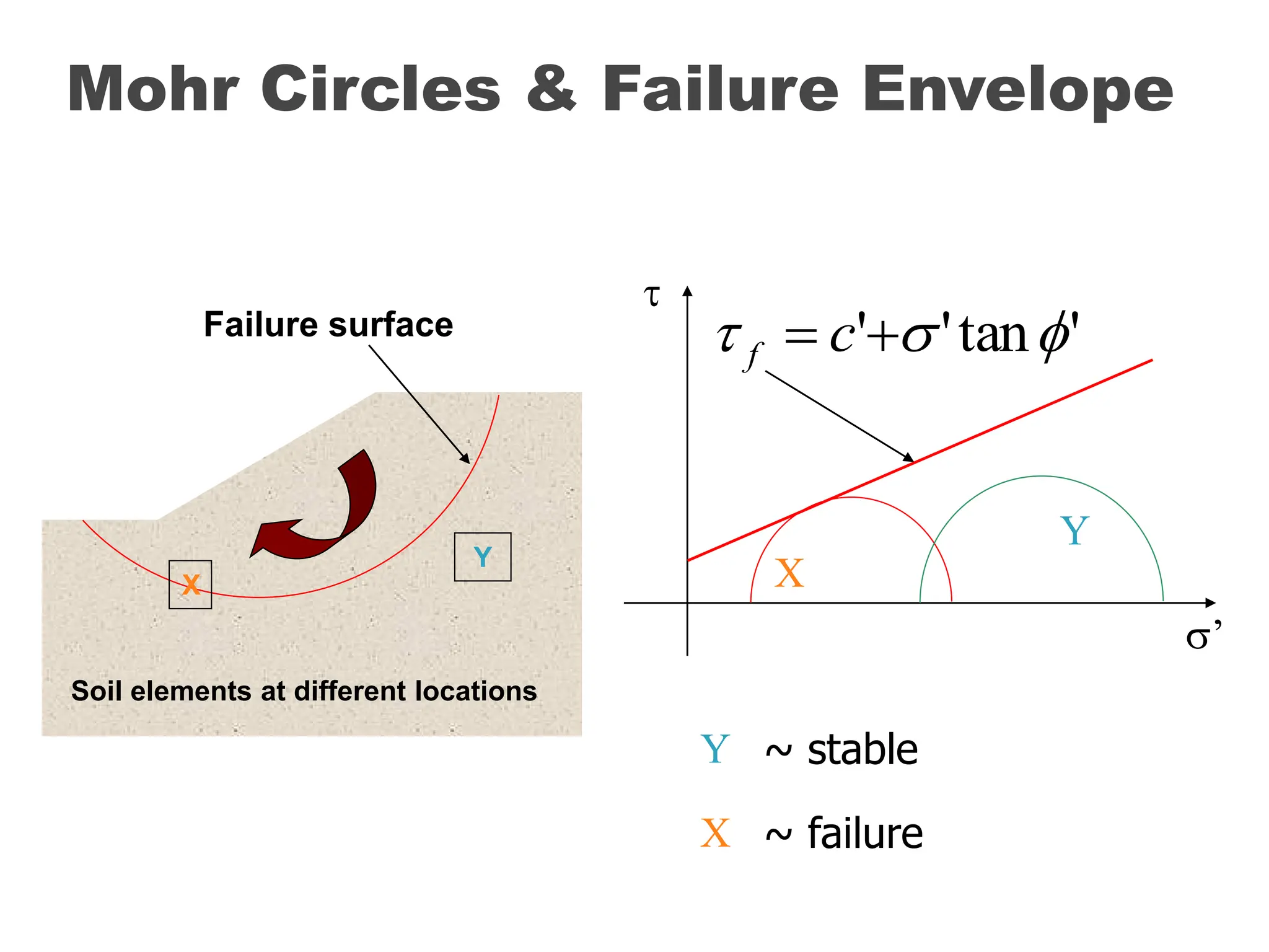
Soil elements atdifferent locations
Failure surface
Mohr Circles & Failure Envelope
X X
X ~ failure
Y
Y
Y ~ stable
’
'
tan
'
'
c
f
16.
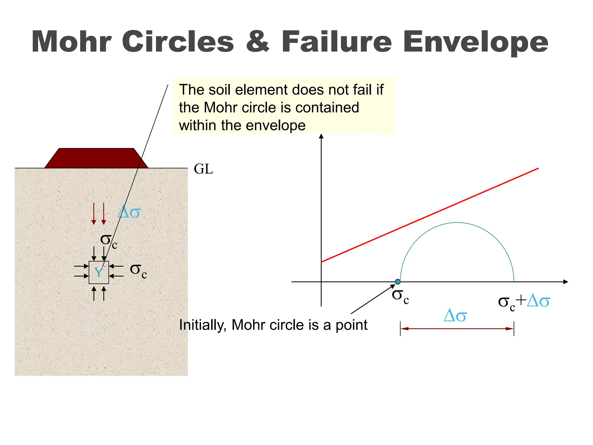
Mohr Circles &Failure Envelope
Y
c
c
c
Initially, Mohr circle is a point
c+
The soil element does not fail if
the Mohr circle is contained
within the envelope
GL
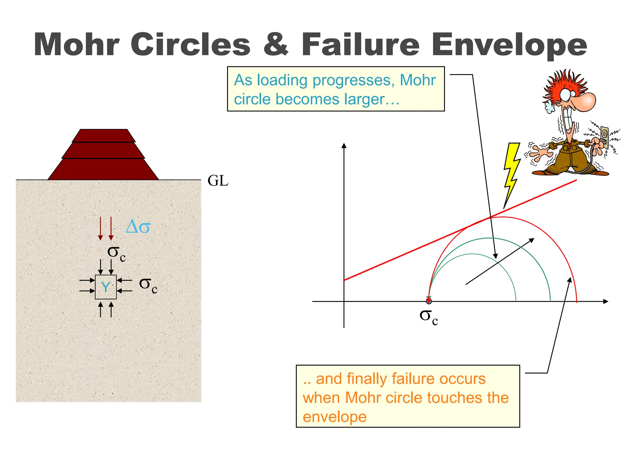
17.
Mohr Circles &Failure Envelope
Y
c
c
c
GL
As loading progresses, Mohr
circle becomes larger…
.. and finally failure occurs
when Mohr circle touches the
envelope
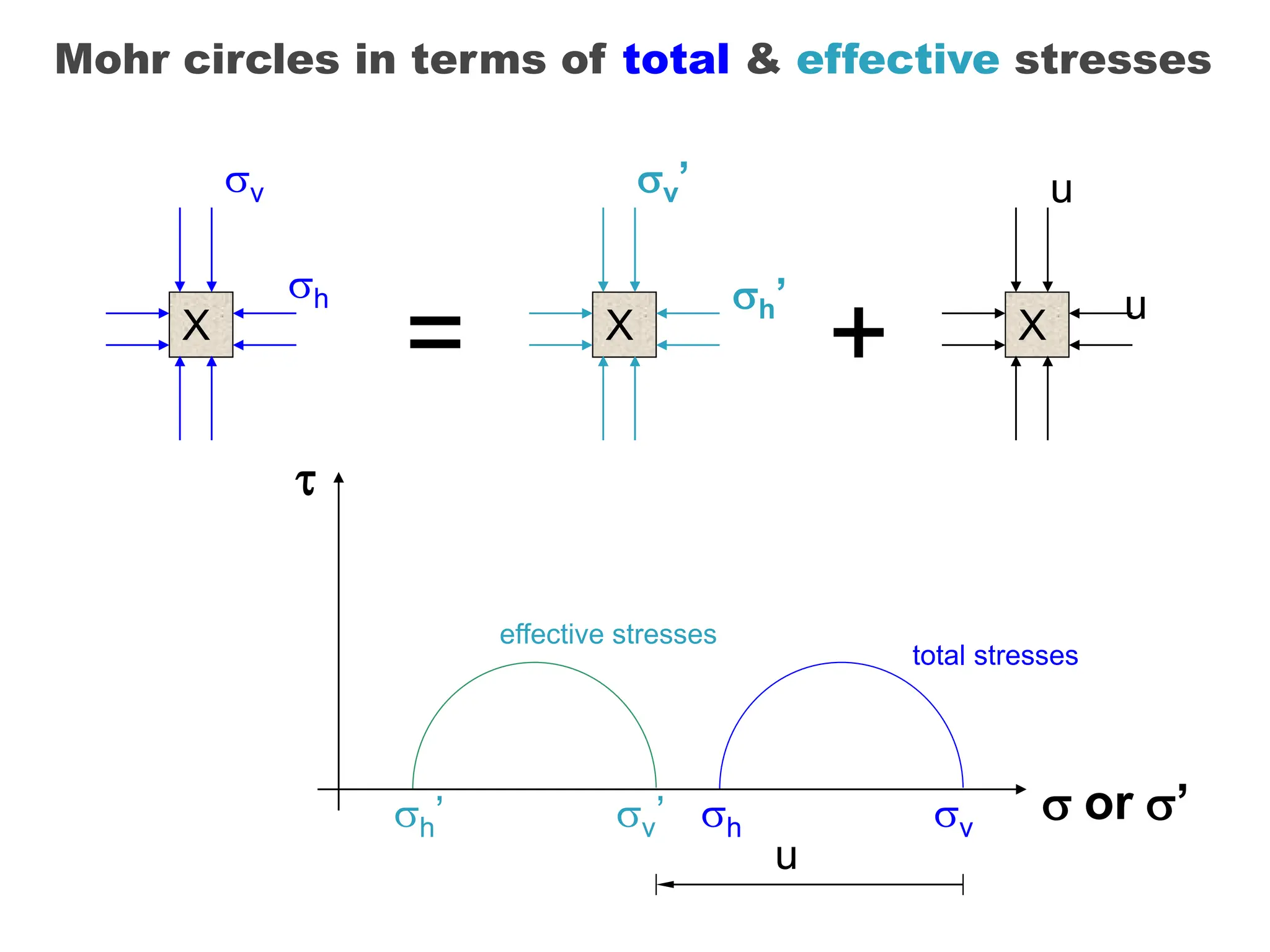
Mohr circles interms of total & effective stresses
= X
v’
h’
X
u
u
+
v’
h’
effective stresses
u
v
h
X
v
h
total stresses
or ’
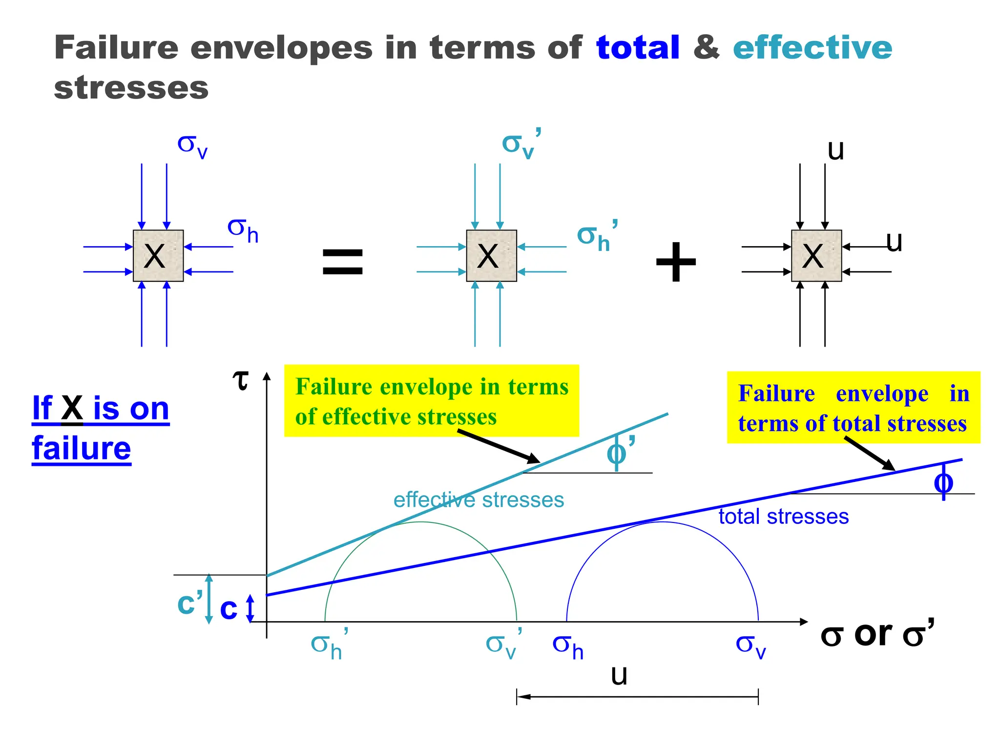
20.
Failure envelopes interms of total & effective
stresses
= X
v’
h’
X
u
u
+
v’
h’
effective stresses
u
v
h
X
v
h
total stresses
or ’
If X is on
failure
c
Failure envelope in
terms of total stresses
’
c’
Failure envelope in terms
of effective stresses
21.
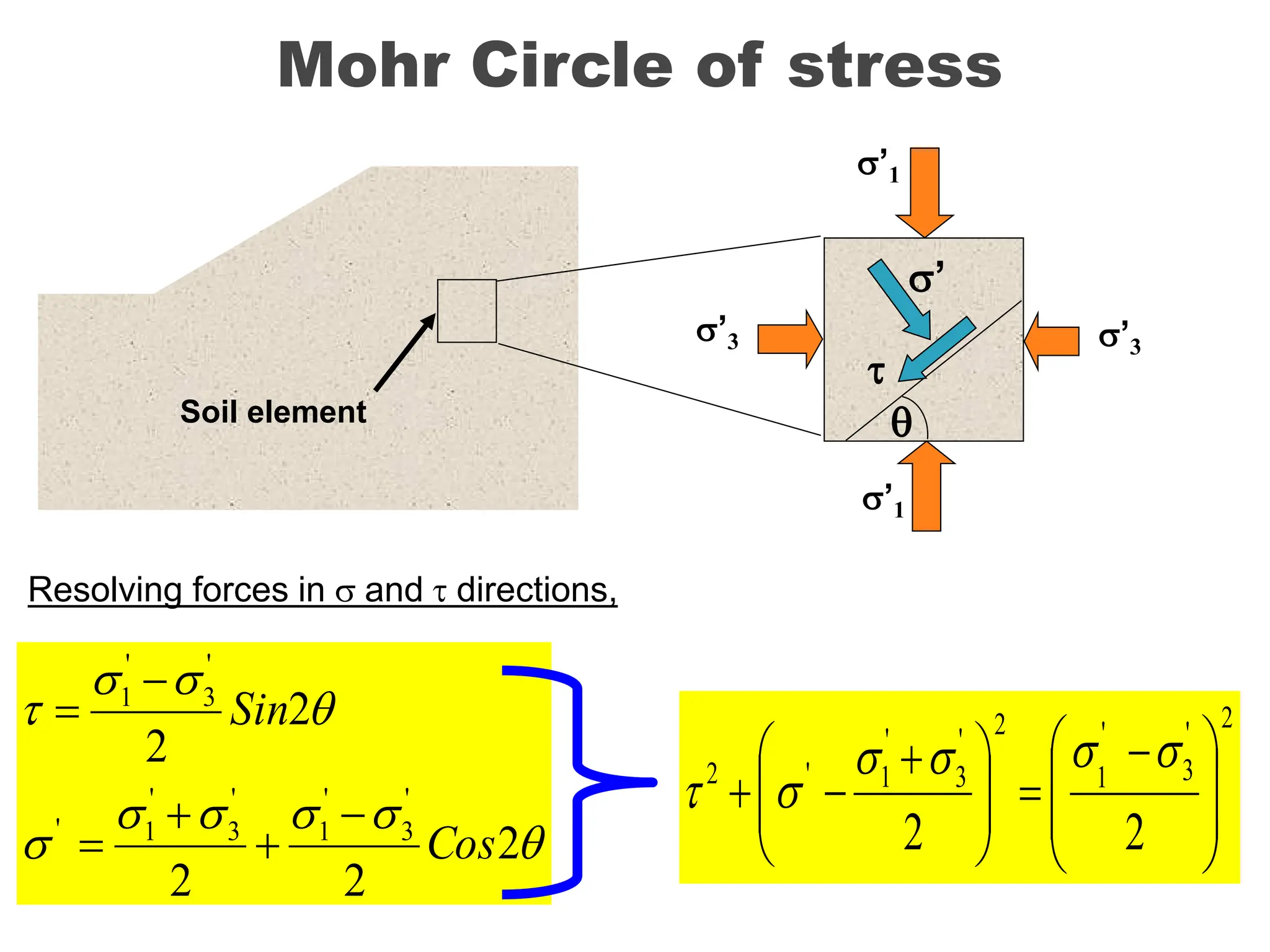
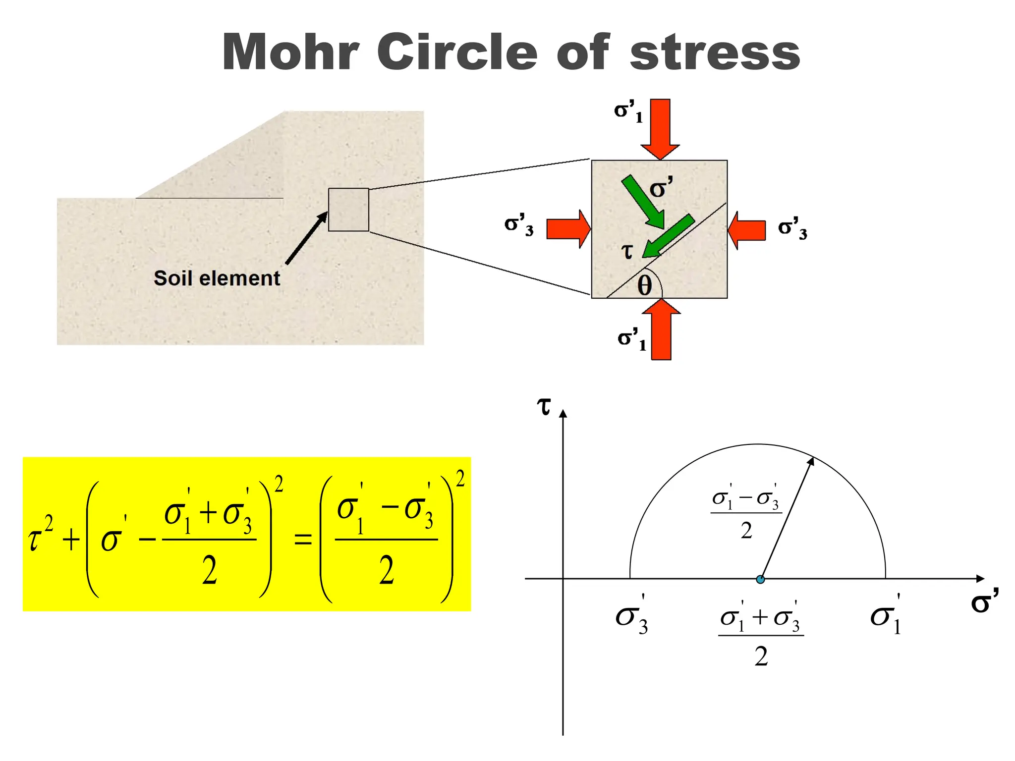
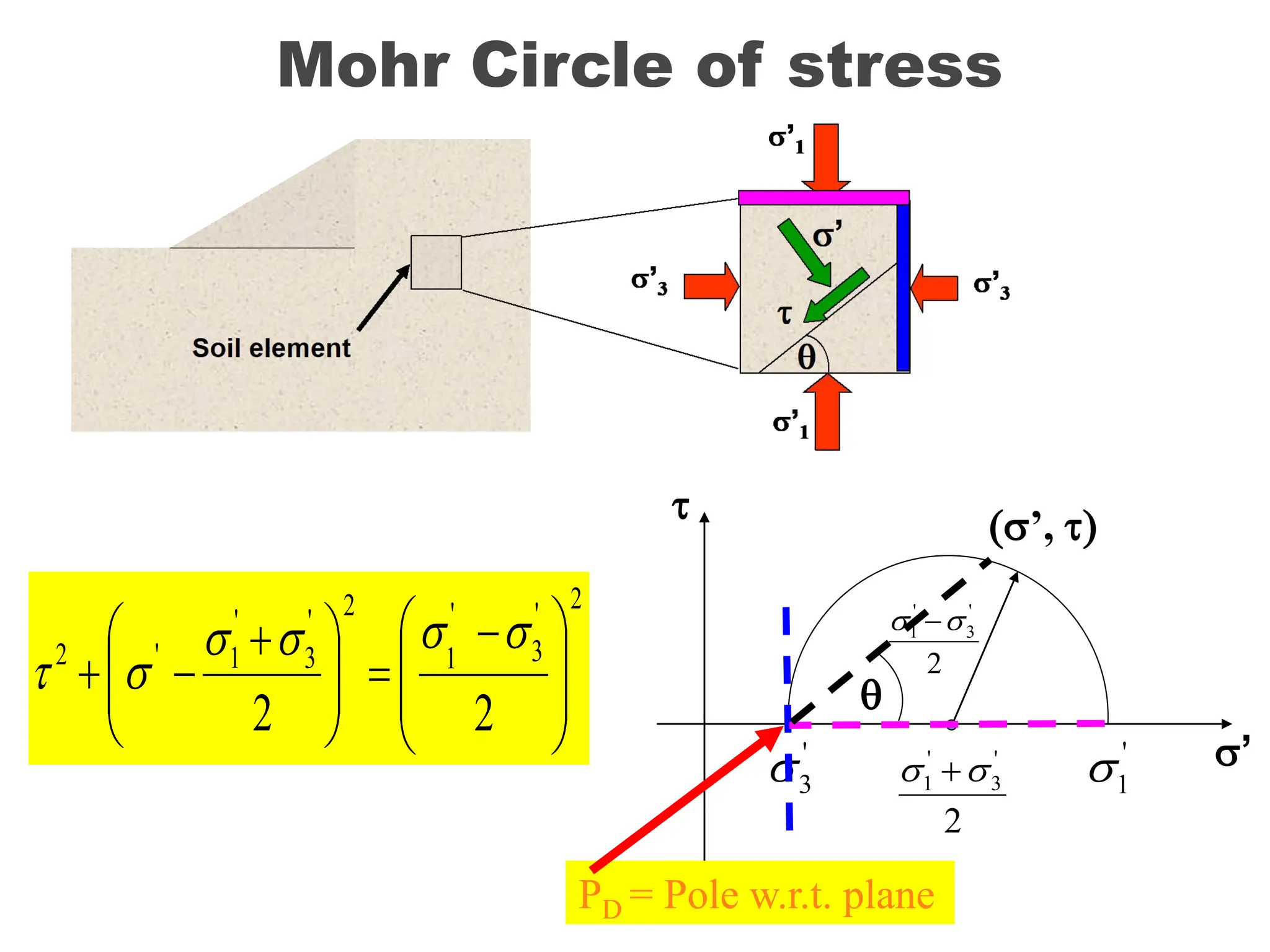
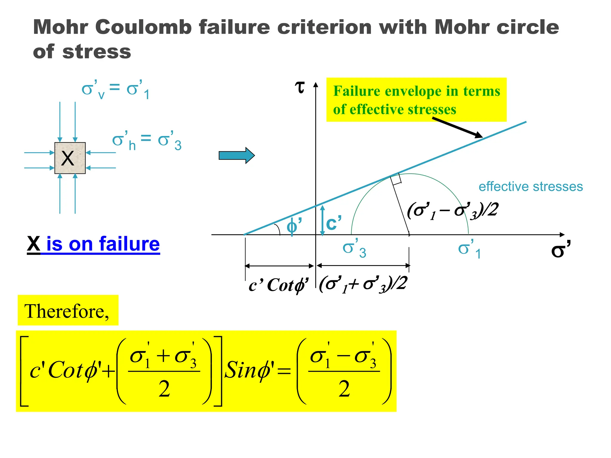
Mohr Coulomb failurecriterion with Mohr circle
of stress
X
’v = ’1
’h = ’3
X is on failure ’1
’3
effective stresses
’
’ c’
Failure envelope in terms
of effective stresses
c’ Cot’ (’1 ’3)/2
(’1 ’3)/2
2
'
2
'
'
'
3
'
1
'
3
'
1
Sin
Cot
c
Therefore,
22.
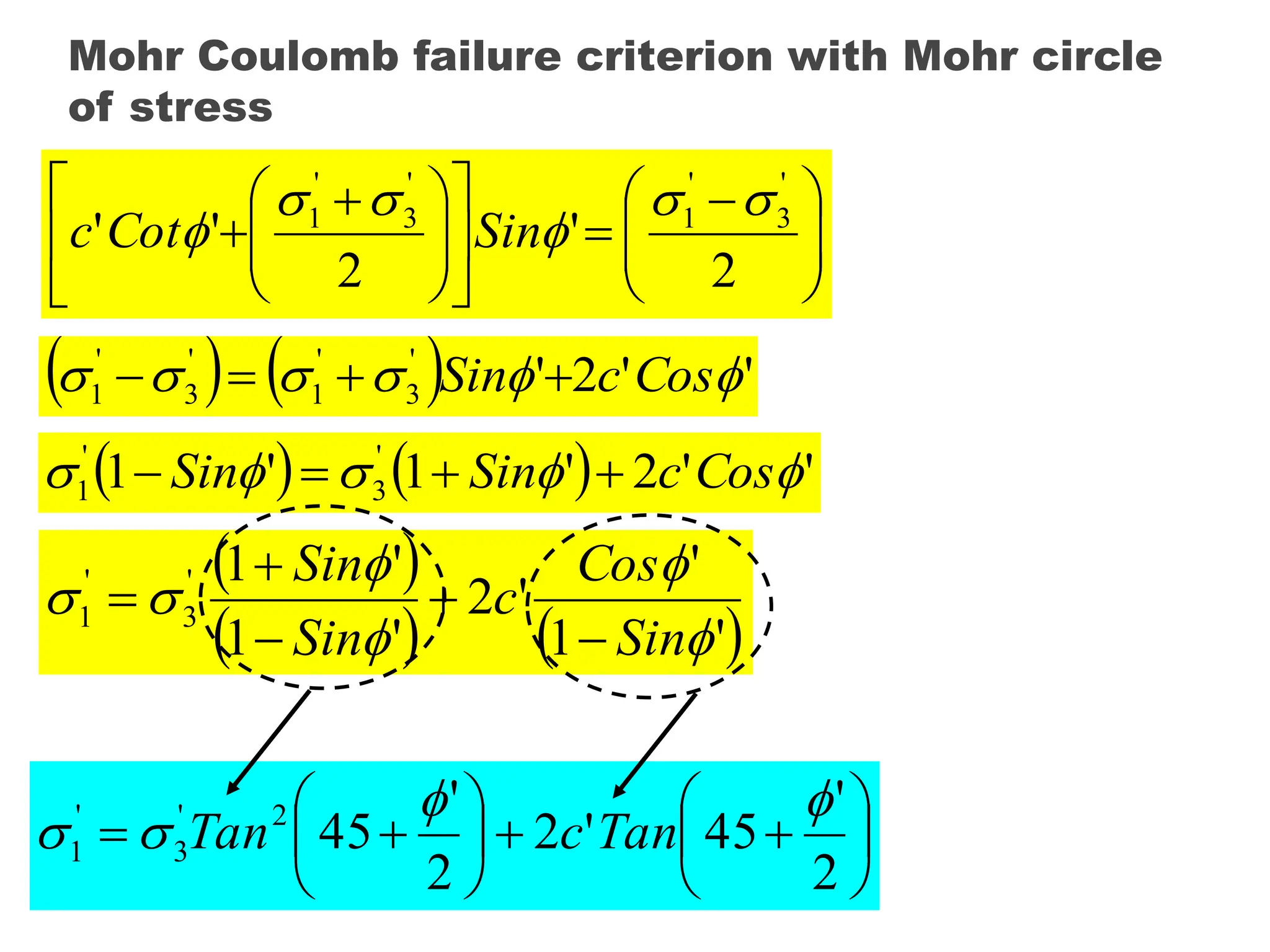
Mohr Coulomb failurecriterion with Mohr circle
of stress
2
'
2
'
'
'
3
'
1
'
3
'
1
Sin
Cot
c
( ) ( ) '
'
2
'
'
3
'
1
'
3
'
1
Cos
c
Sin
( ) ( ) '
'
2
'
1
'
1 '
3
'
1
Cos
c
Sin
Sin
( )
( ) ( )
'
1
'
'
2
'
1
'
1
'
3
'
1
Sin
Cos
c
Sin
Sin
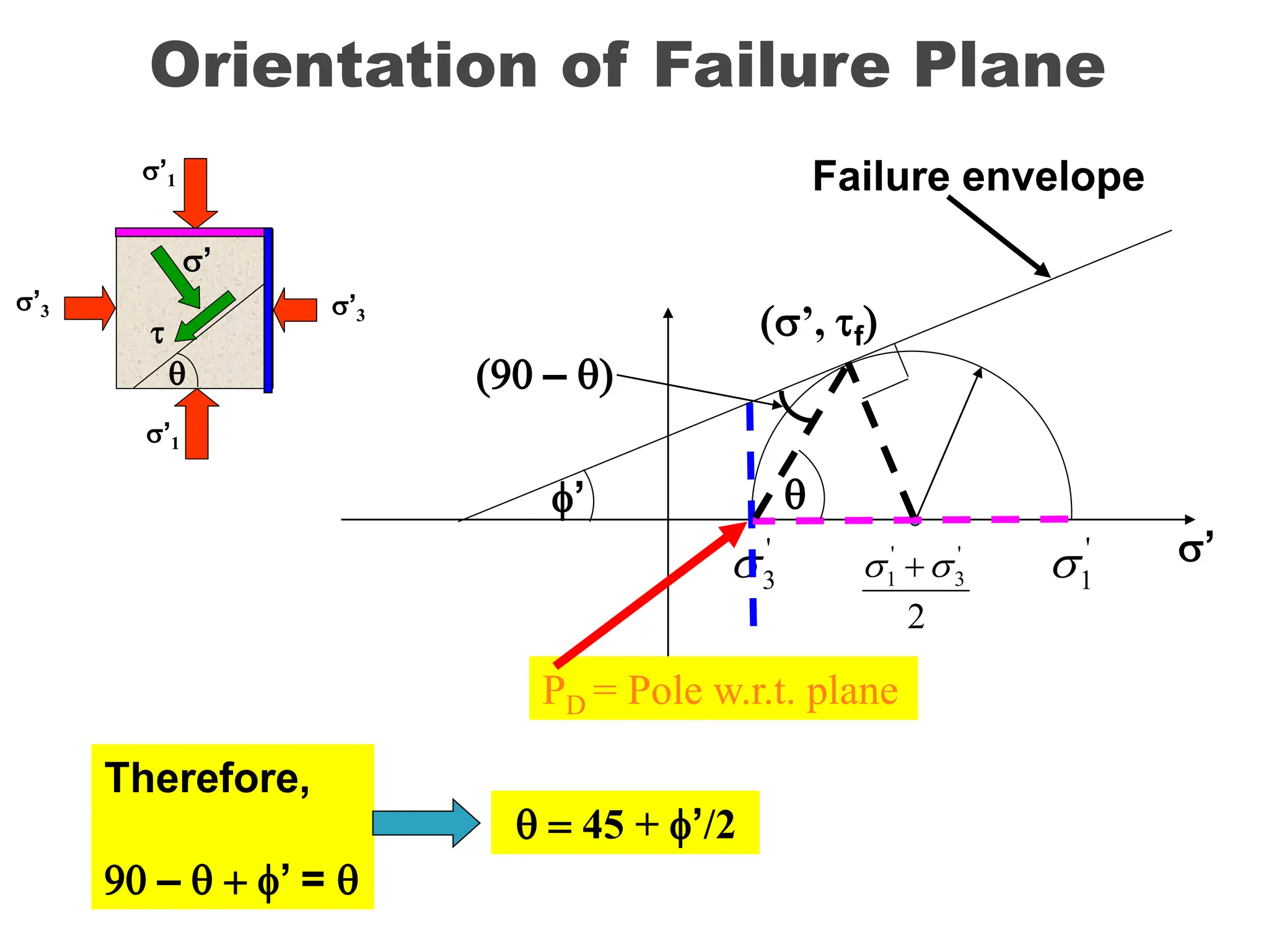
2
'
45
'
2
2
'
45
2
'
3
'
1
Tan
c
Tan
23.
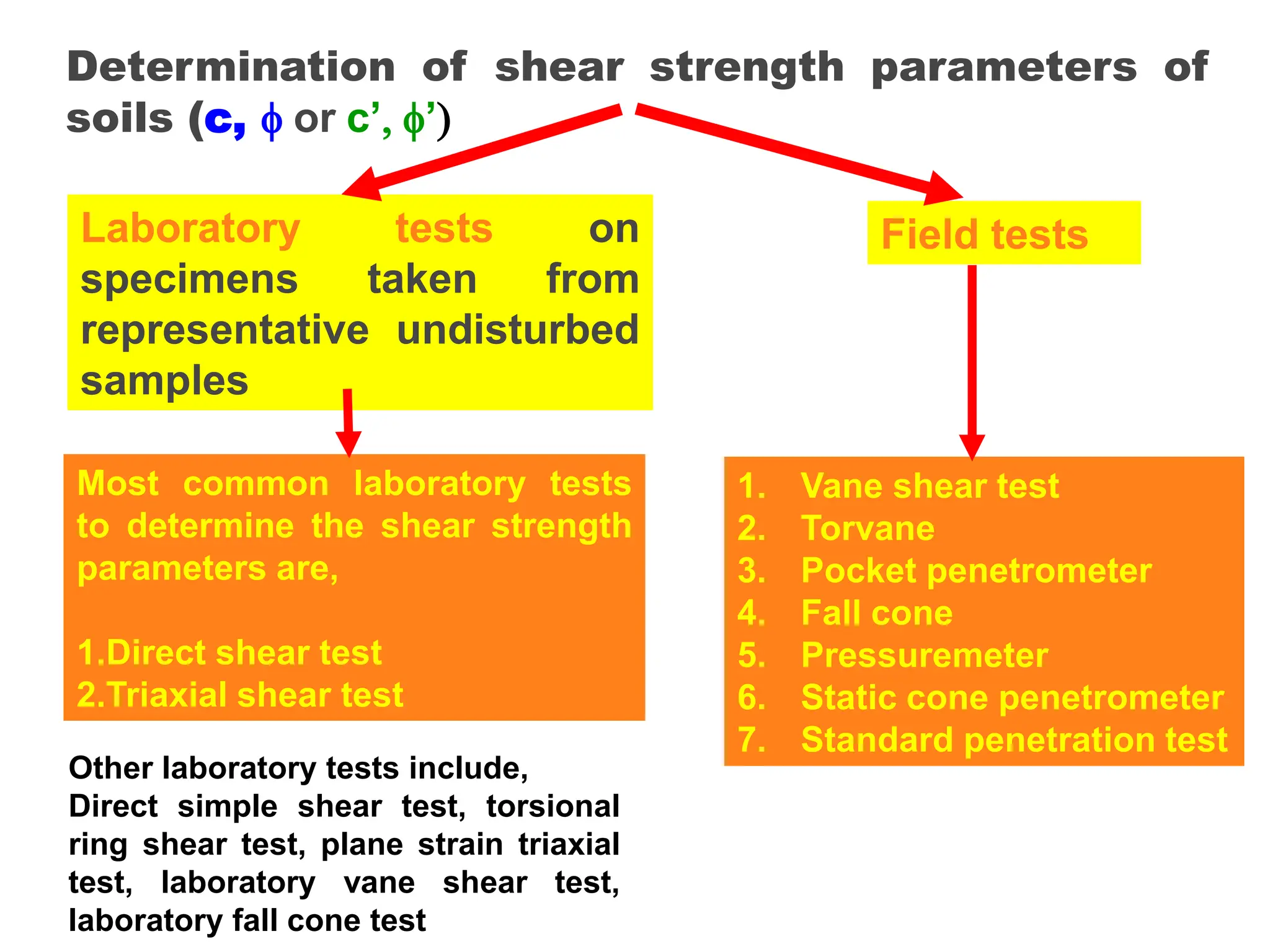
Other laboratory testsinclude,
Direct simple shear test, torsional
ring shear test, plane strain triaxial
test, laboratory vane shear test,
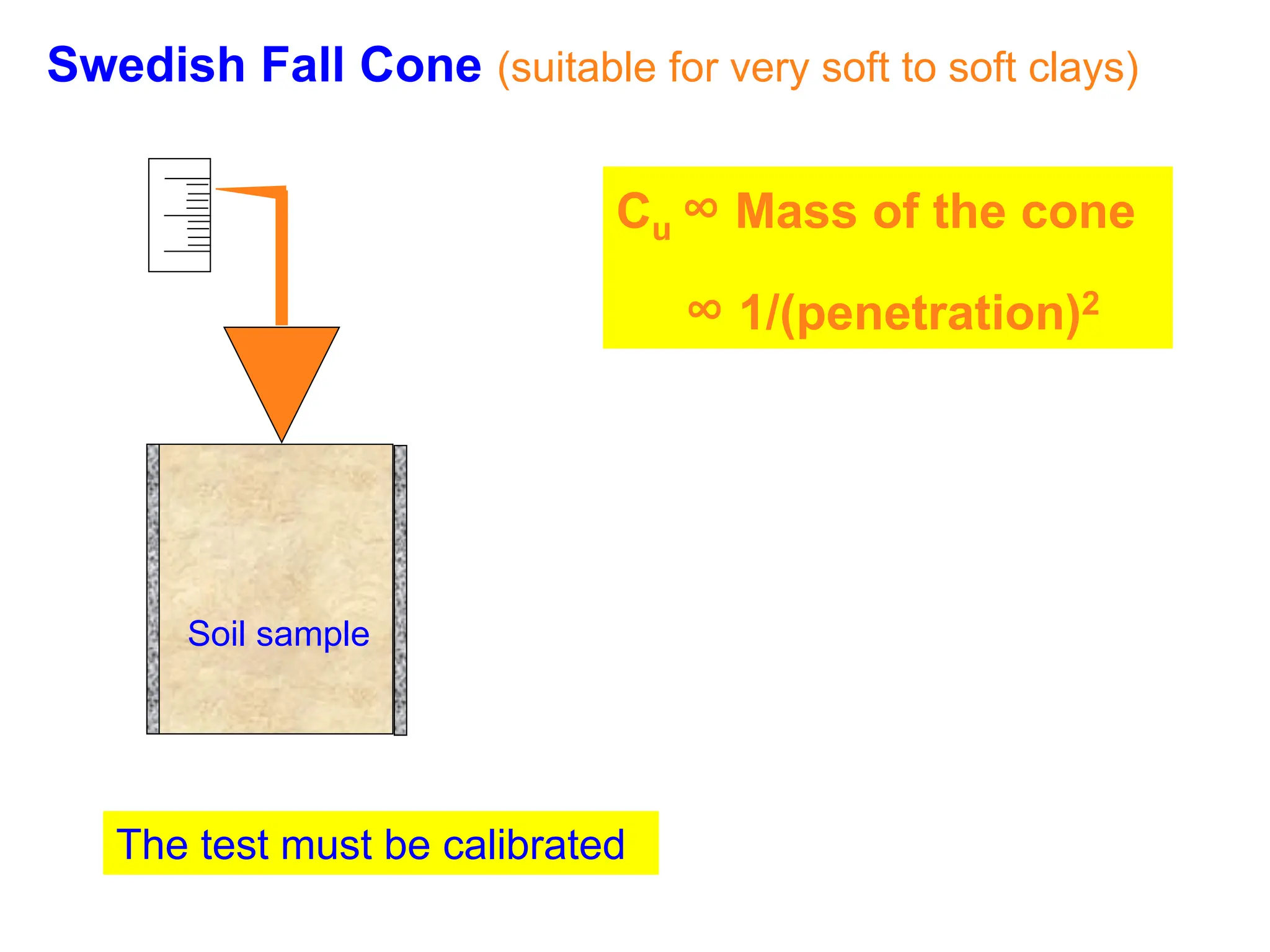
laboratory fall cone test
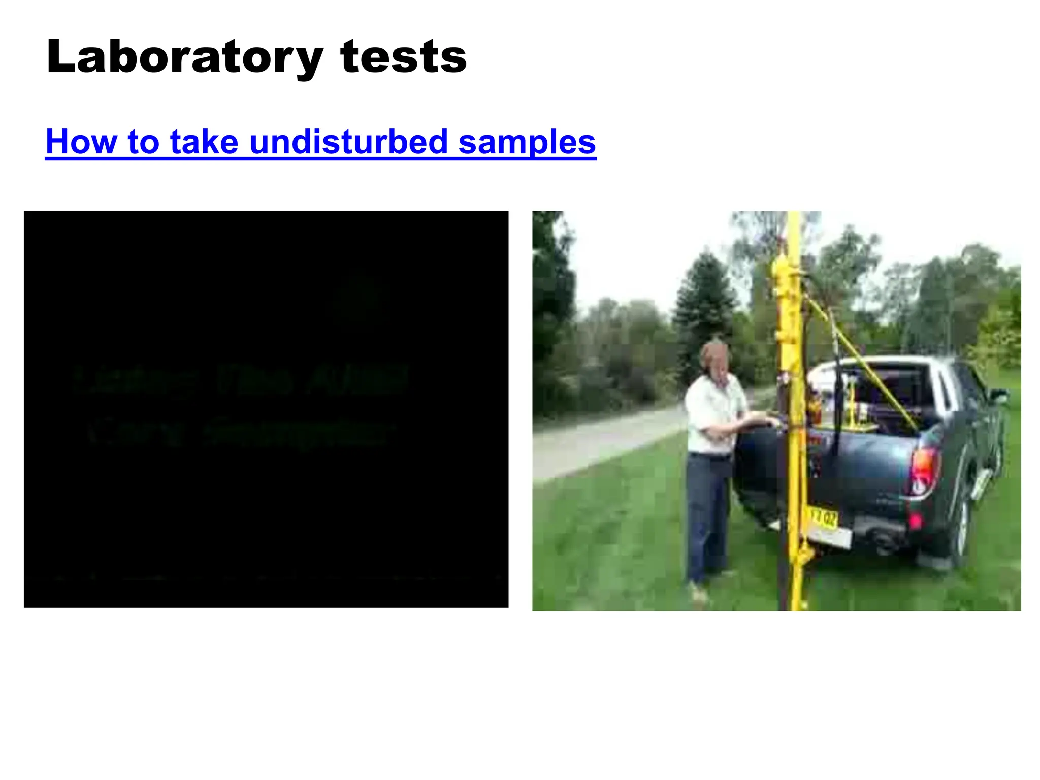
Determination of shear strength parameters of
soils (c, or c’, ’)
Laboratory tests on
specimens taken from
representative undisturbed
samples
Field tests
Most common laboratory tests
to determine the shear strength
parameters are,
1.Direct shear test
2.Triaxial shear test
1. Vane shear test
2. Torvane
3. Pocket penetrometer
4. Fall cone
5. Pressuremeter
6. Static cone penetrometer
7. Standard penetration test
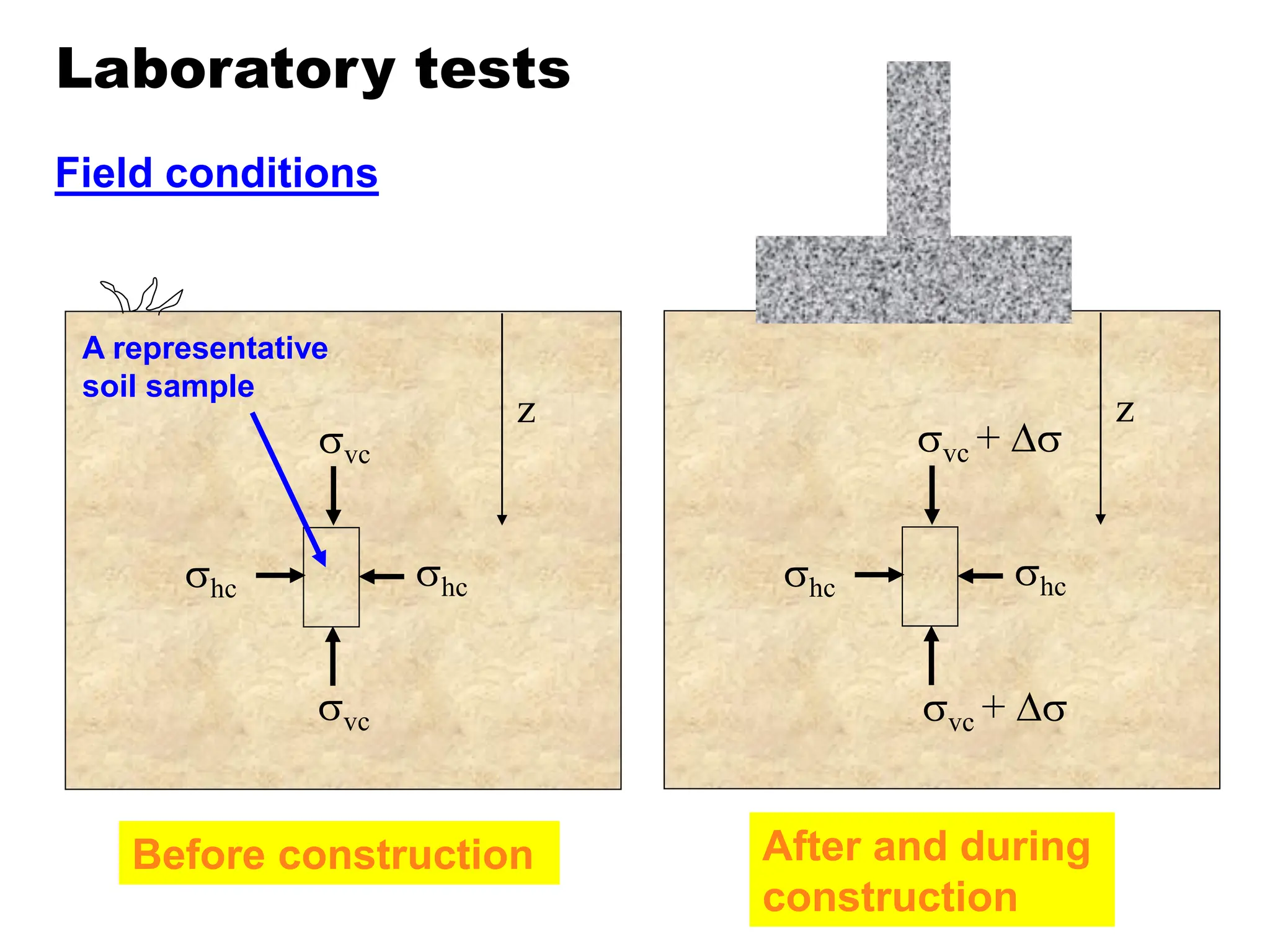
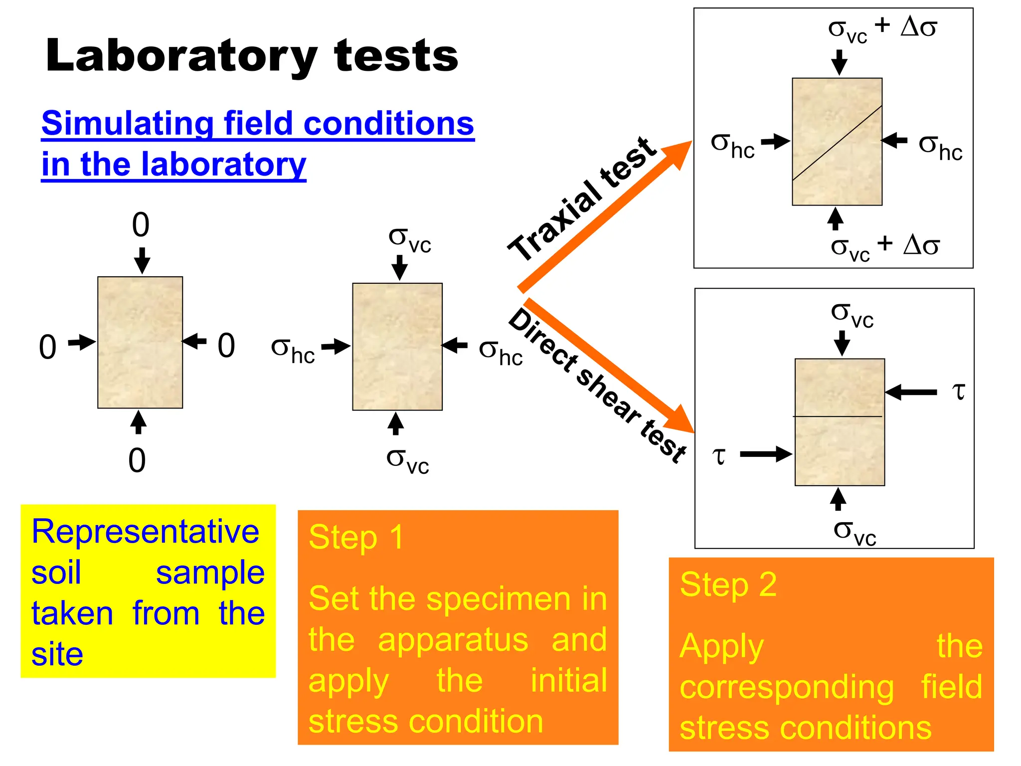
Laboratory tests
Simulating fieldconditions
in the laboratory
Step 1
Set the specimen in
the apparatus and
apply the initial
stress condition
vc
vc
hc
hc
Representative
soil sample
taken from the
site
0
0
0
0
Step 2
Apply the
corresponding field
stress conditions
vc +
hc
hc
vc +
vc
vc
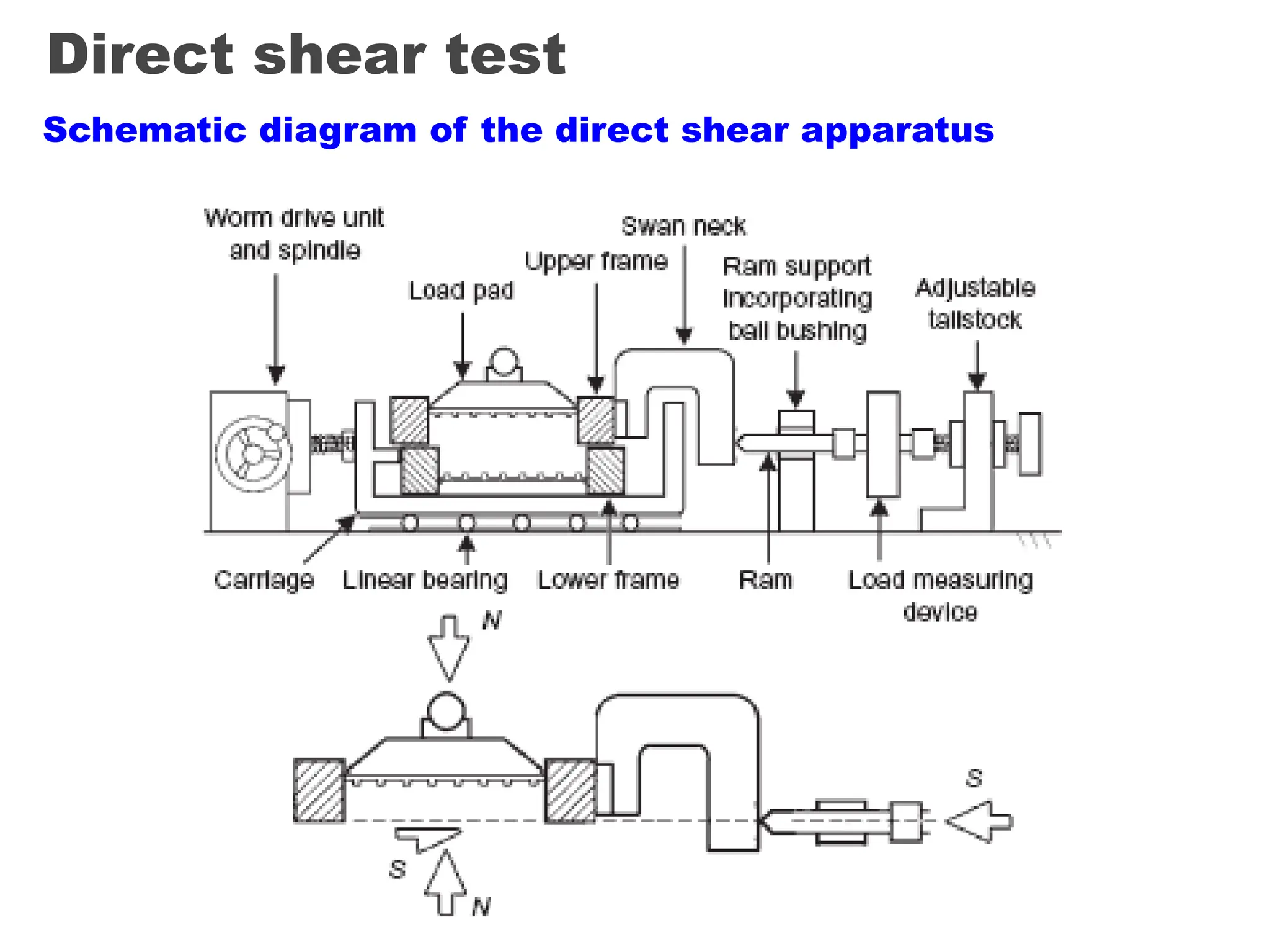
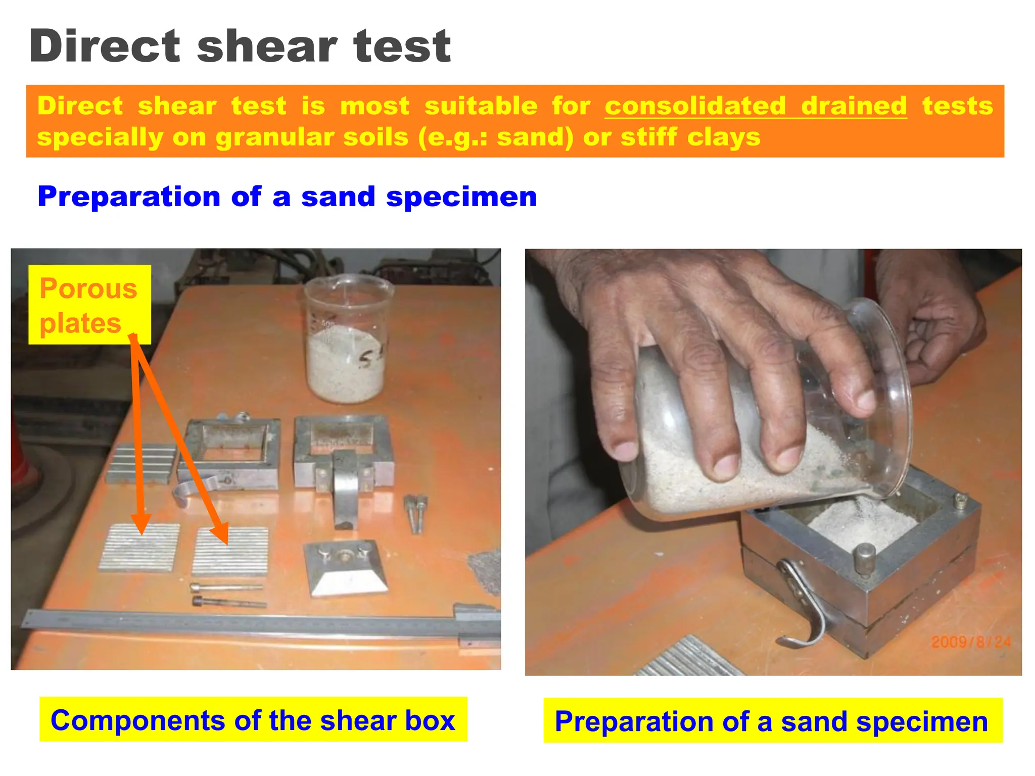
Direct shear test
Preparationof a sand specimen
Components of the shear box Preparation of a sand specimen
Porous
plates
Direct shear test is most suitable for consolidated drained tests
specially on granular soils (e.g.: sand) or stiff clays
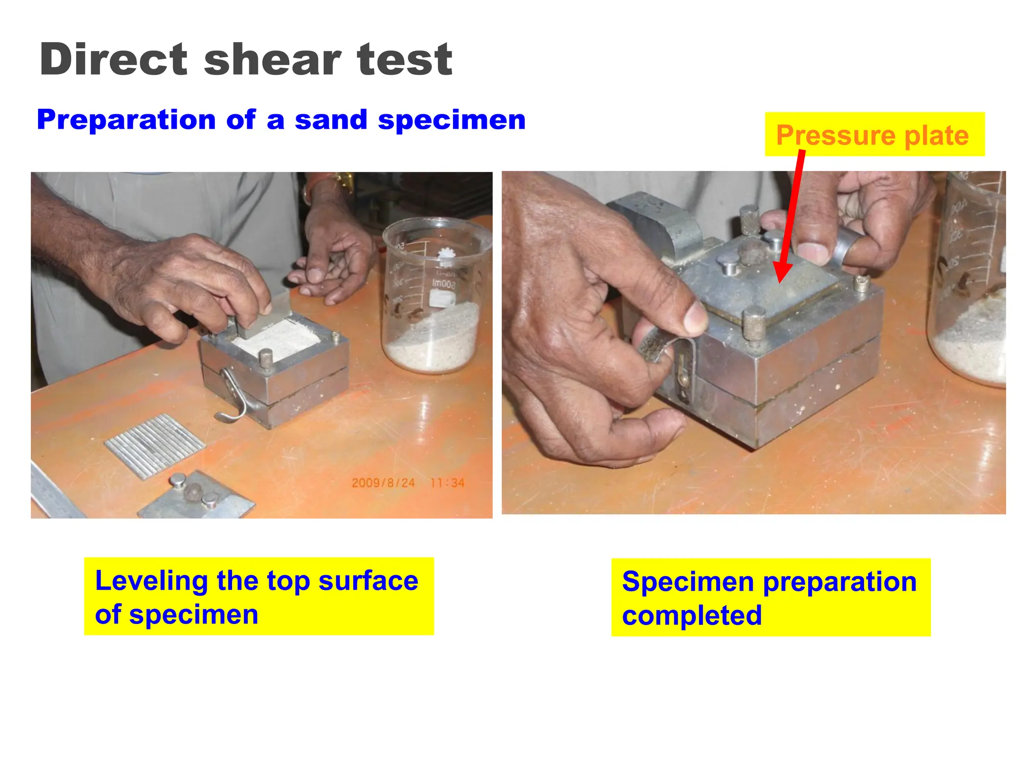
29.
Direct shear test
Levelingthe top surface
of specimen
Preparation of a sand specimen
Specimen preparation
completed
Pressure plate
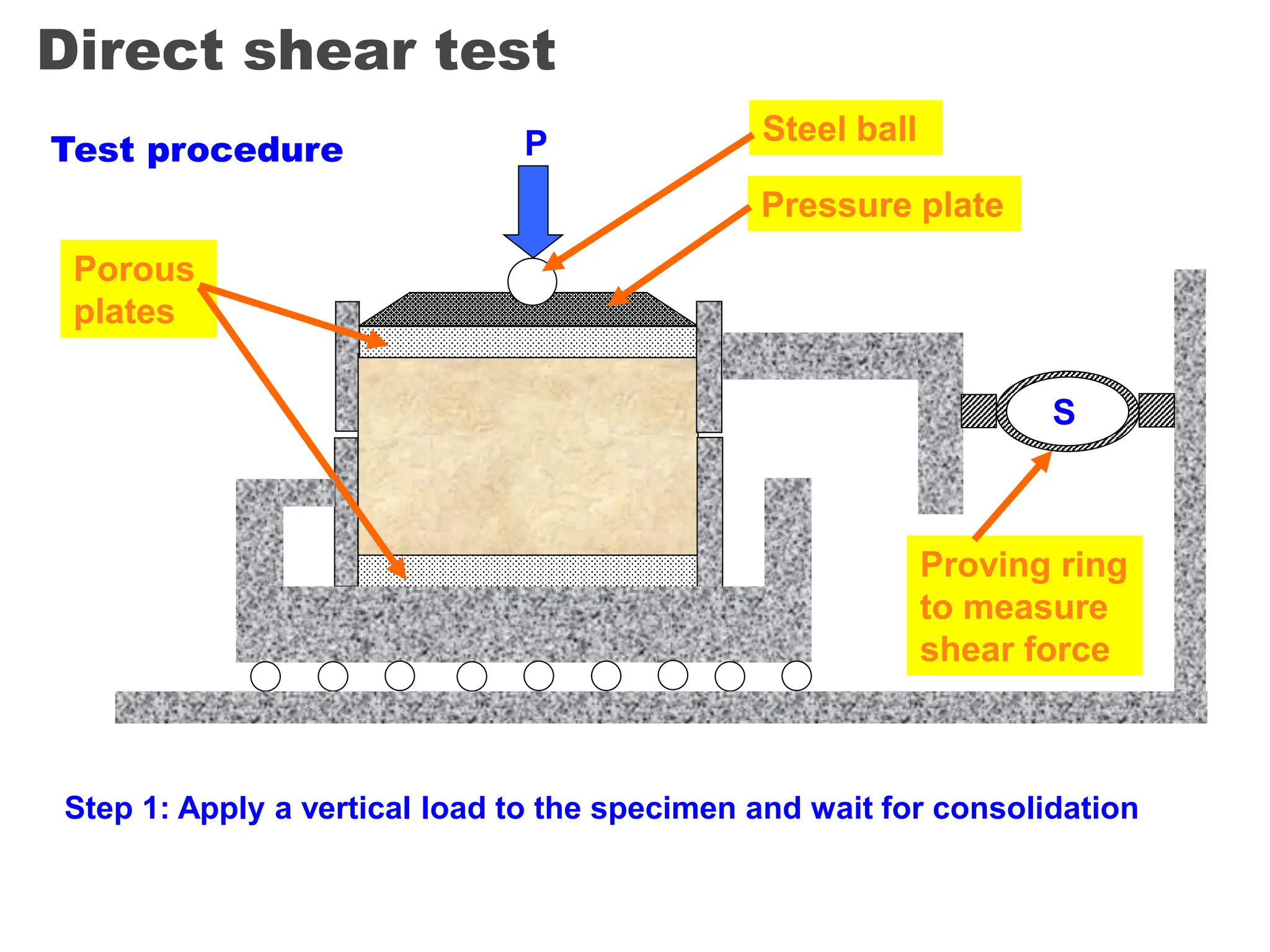
30.
Direct shear test
Testprocedure
Porous
plates
Pressure plate
Steel ball
Step 1: Apply a vertical load to the specimen and wait for consolidation
P
Proving ring
to measure
shear force
S
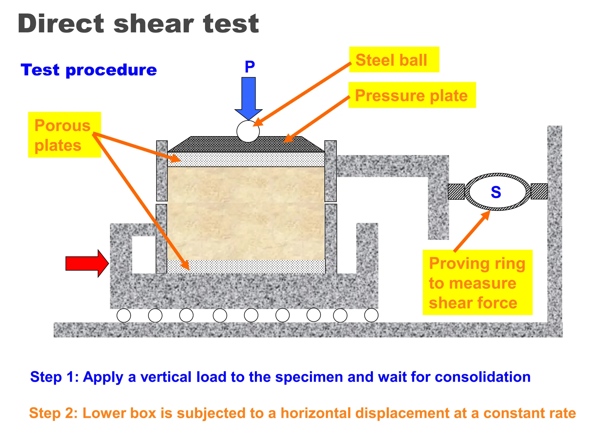
31.
Direct shear test
Step2: Lower box is subjected to a horizontal displacement at a constant rate
Step 1: Apply a vertical load to the specimen and wait for consolidation
P
Test procedure
Pressure plate
Steel ball
Proving ring
to measure
shear force
S
Porous
plates
32.
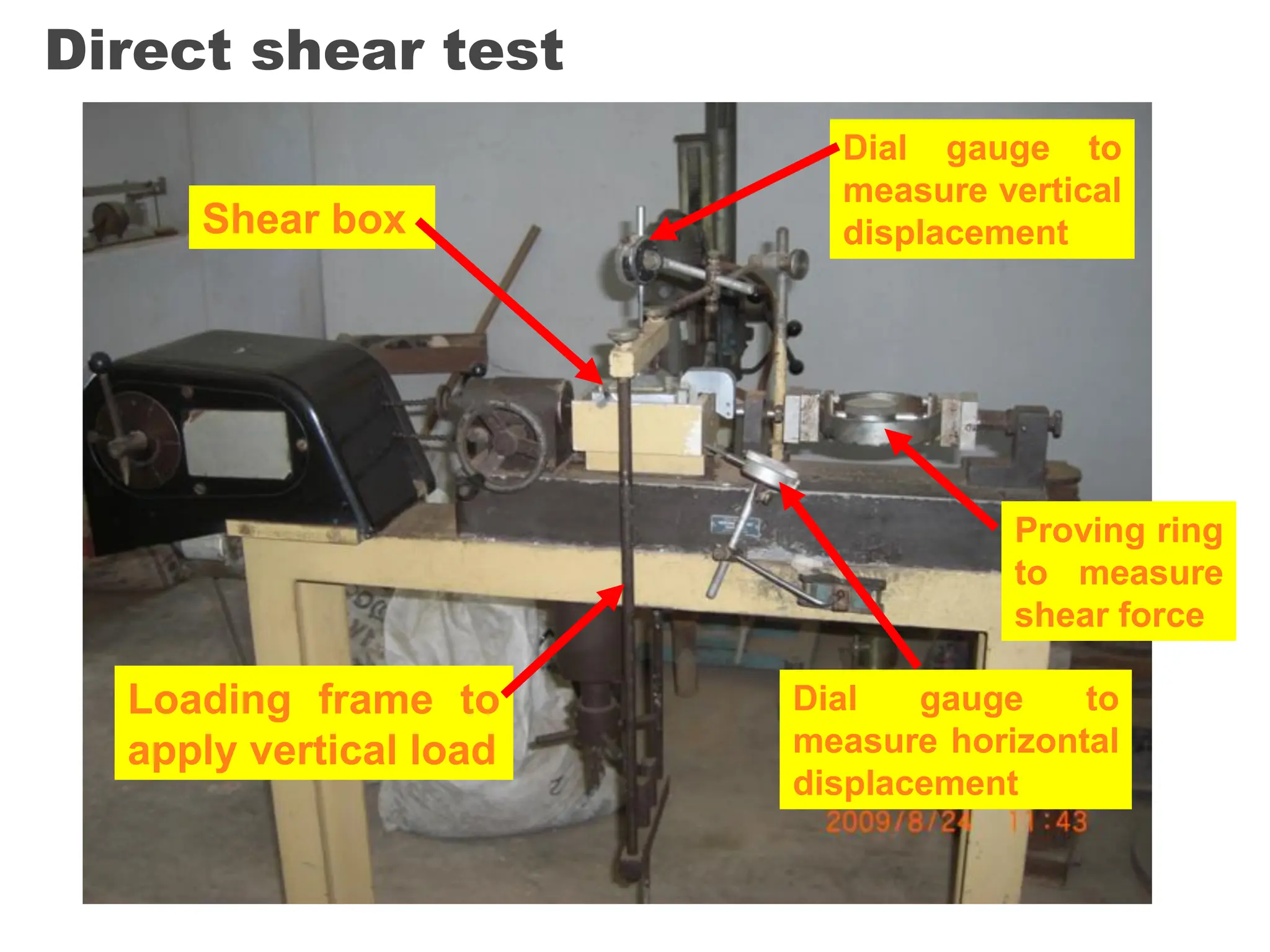
Direct shear test
Shearbox
Loading frame to
apply vertical load
Dial gauge to
measure vertical
displacement
Dial gauge to
measure horizontal
displacement
Proving ring
to measure
shear force
33.
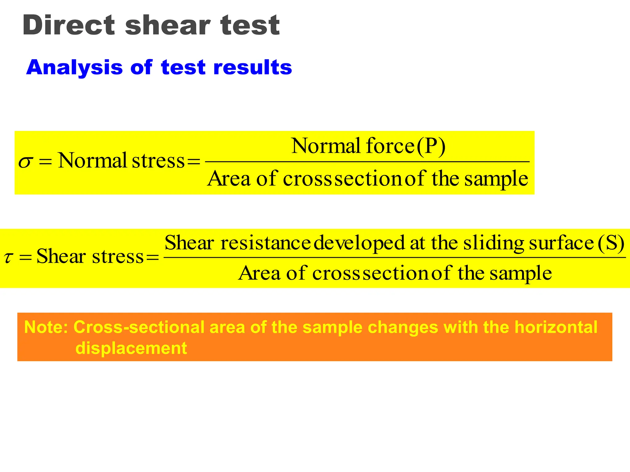
Direct shear test
Analysisof test results
sample
the
of
section
cross
of
Area
(P)
force
Normal
stress
Normal
sample
the
of
section
cross
of
Area
(S)
surface
sliding
at the
developed
resistance
Shear
stress
Shear
Note: Cross-sectional area of the sample changes with the horizontal
displacement
34.
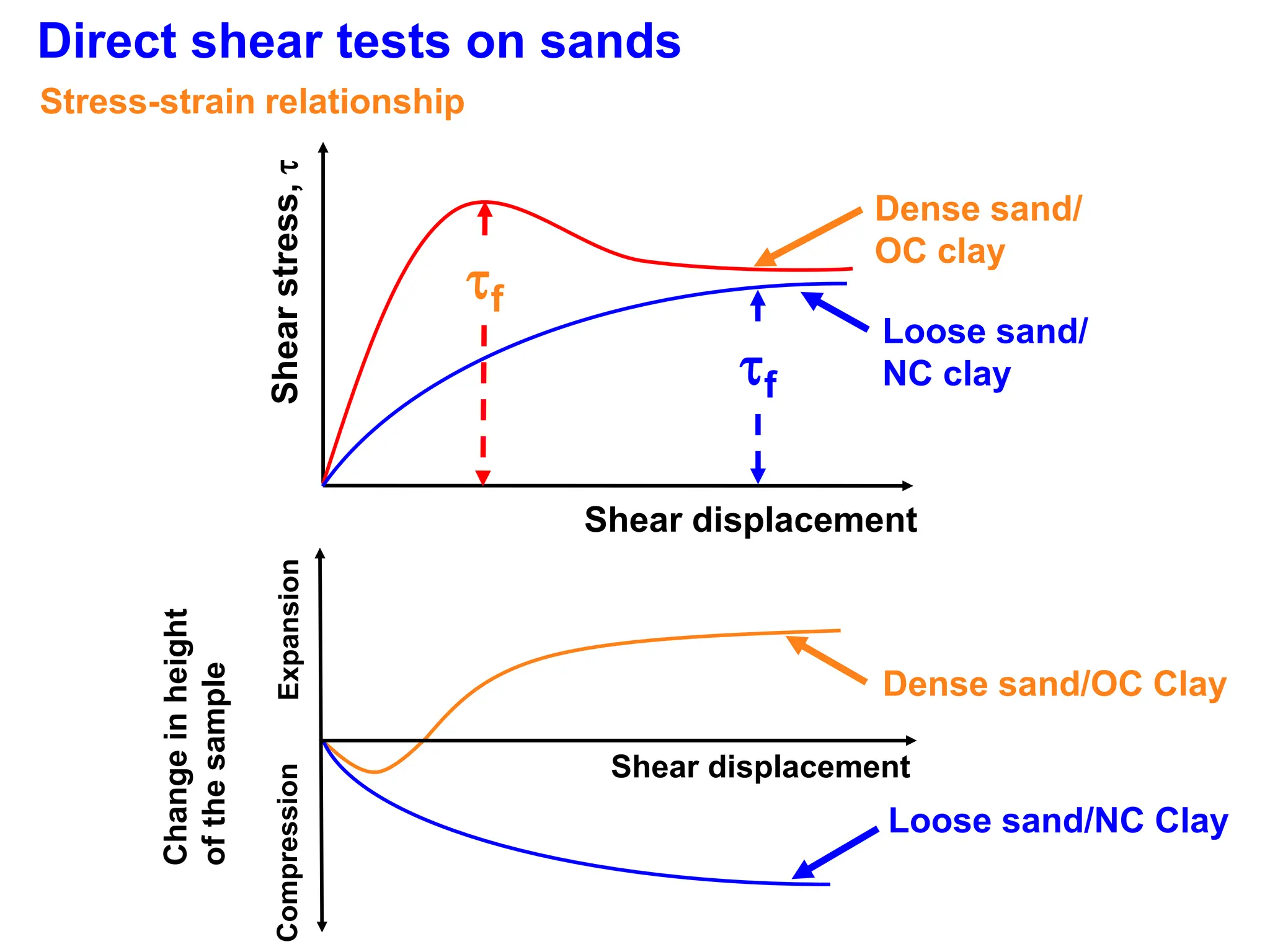
Direct shear testson sands
Shear
stress,
Shear displacement
Dense sand/
OC clay
f
Loose sand/
NC clay
f
Dense sand/OC Clay
Loose sand/NC Clay
Change
in
height
of
the
sample
Expansion
Compression
Shear displacement
Stress-strain relationship
35.
f1
Normal stress =1
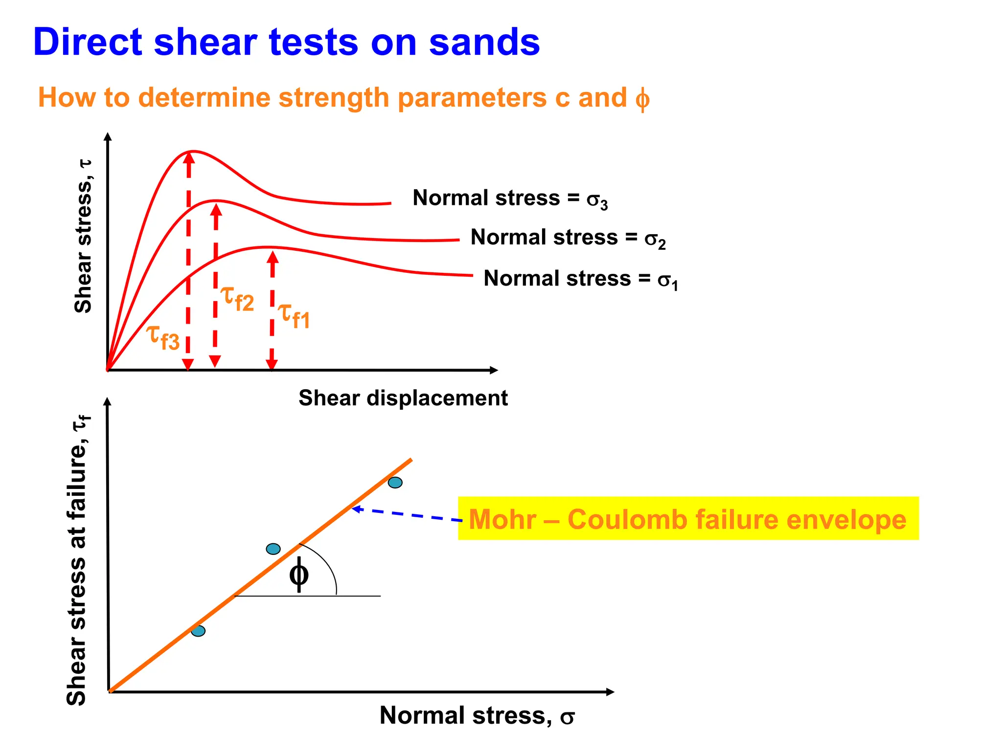
Direct shear tests on sands
How to determine strength parameters c and
Shear
stress,
Shear displacement
f2
Normal stress = 2
f3
Normal stress = 3
Shear
stress
at
failure,
f
Normal stress,
Mohr – Coulomb failure envelope
36.
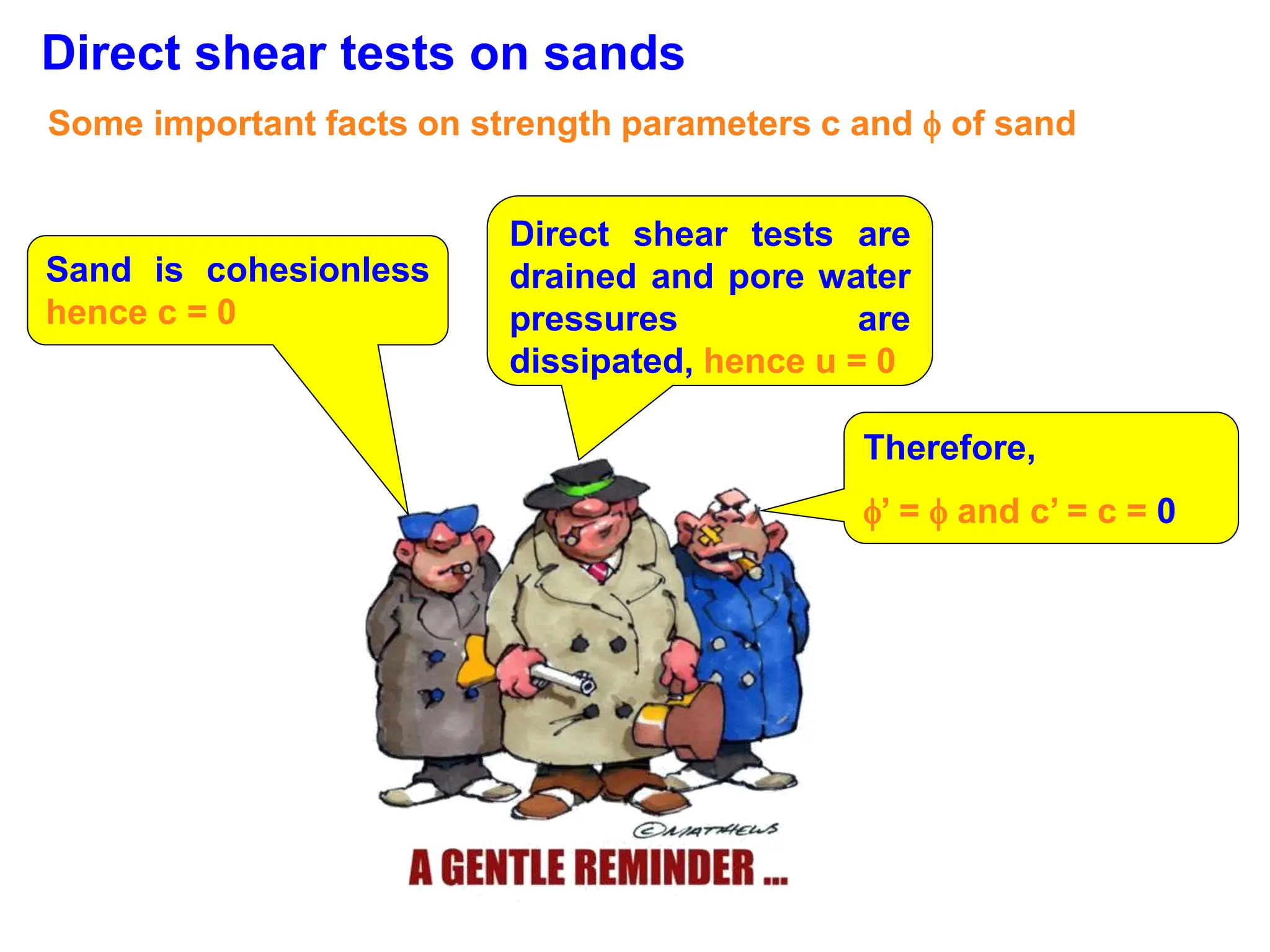
Direct shear testson sands
Some important facts on strength parameters c and of sand
Sand is cohesionless
hence c = 0
Direct shear tests are
drained and pore water
pressures are
dissipated, hence u = 0
Therefore,
’ = and c’ = c = 0
37.
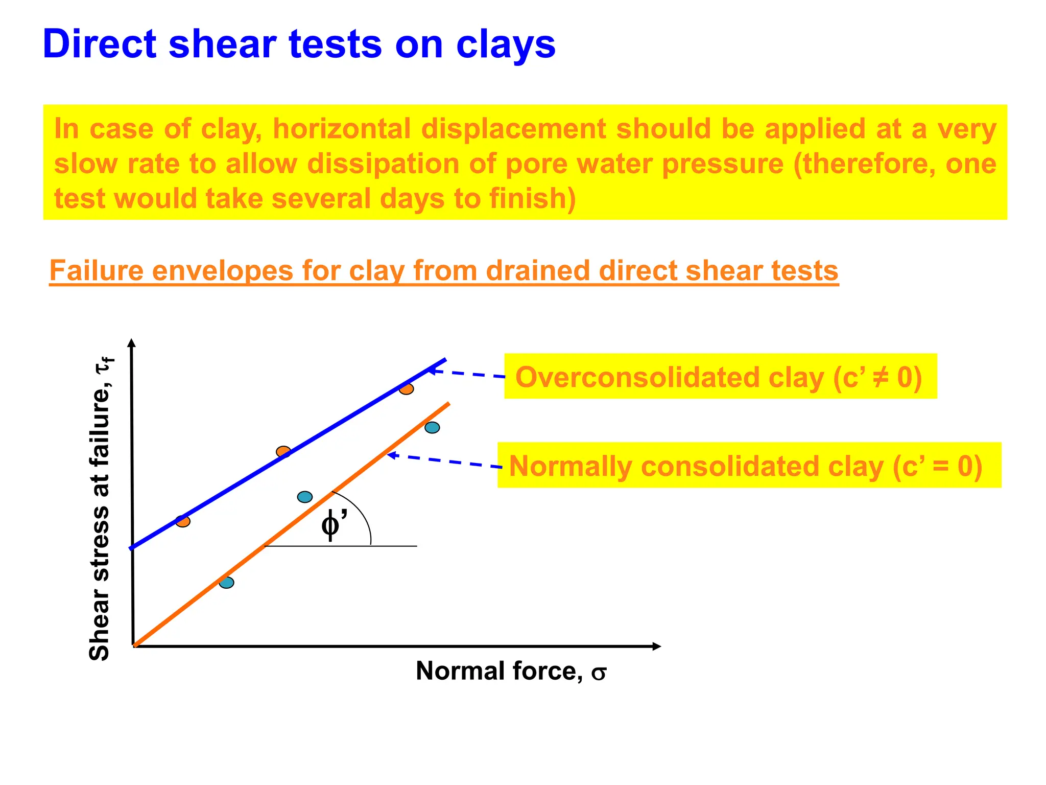
Direct shear testson clays
Failure envelopes for clay from drained direct shear tests
Shear
stress
at
failure,
f
Normal force,
’
Normally consolidated clay (c’ = 0)
In case of clay, horizontal displacement should be applied at a very
slow rate to allow dissipation of pore water pressure (therefore, one
test would take several days to finish)
Overconsolidated clay (c’ ≠ 0)
38.
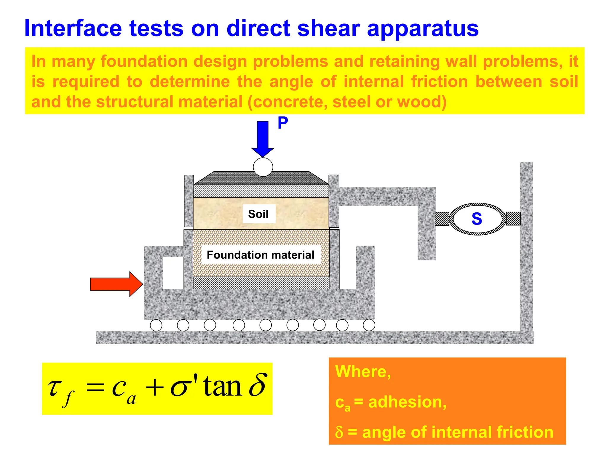
Interface tests ondirect shear apparatus
In many foundation design problems and retaining wall problems, it
is required to determine the angle of internal friction between soil
and the structural material (concrete, steel or wood)
tan
'
a
f c
Where,
ca = adhesion,
= angle of internal friction
Foundation material
Soil
P
S
Foundation material
Soil
P
S
39.
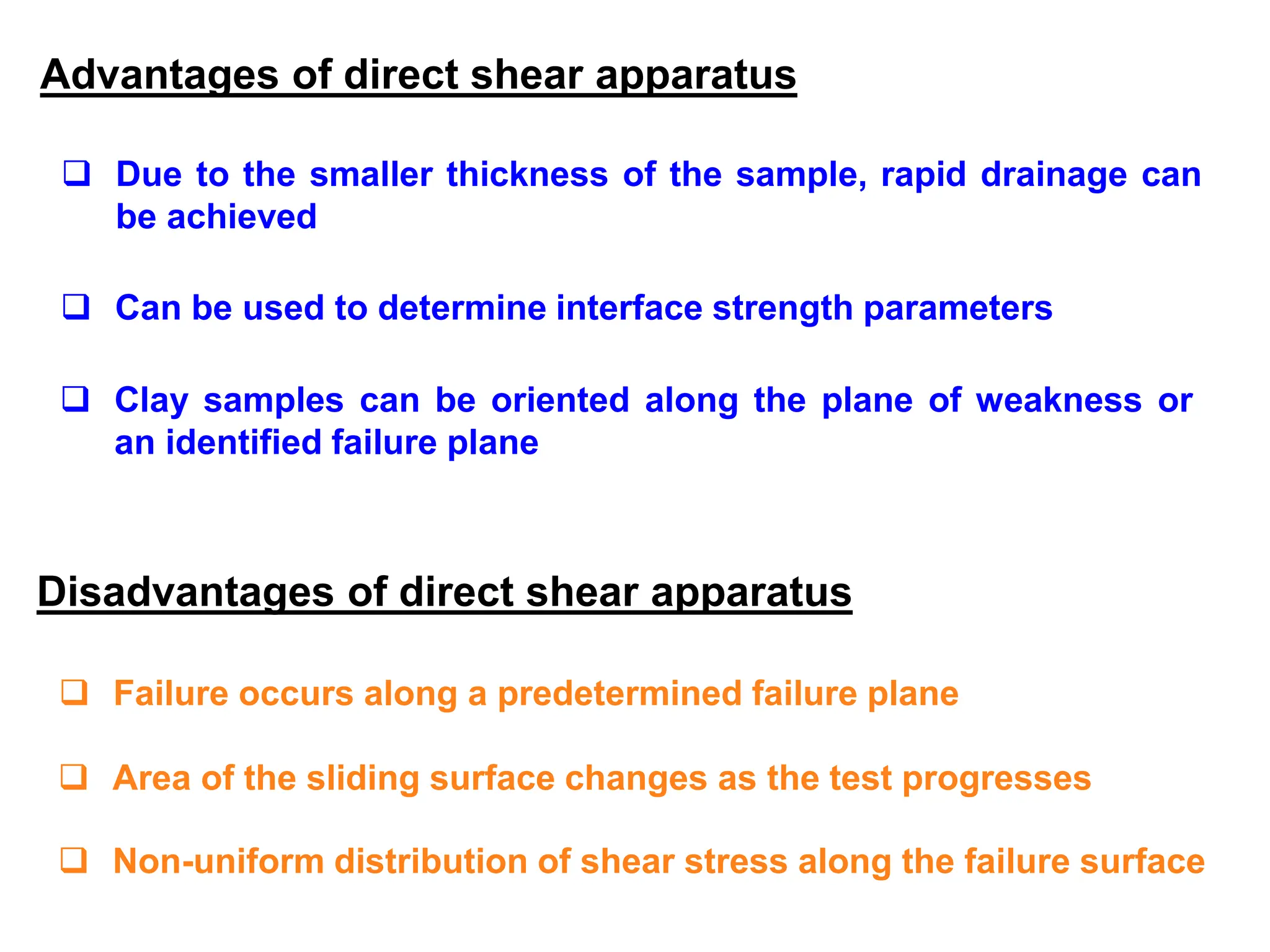
Advantages of directshear apparatus
Due to the smaller thickness of the sample, rapid drainage can
be achieved
Can be used to determine interface strength parameters
Clay samples can be oriented along the plane of weakness or
an identified failure plane
Disadvantages of direct shear apparatus
Failure occurs along a predetermined failure plane
Area of the sliding surface changes as the test progresses
Non-uniform distribution of shear stress along the failure surface
41.
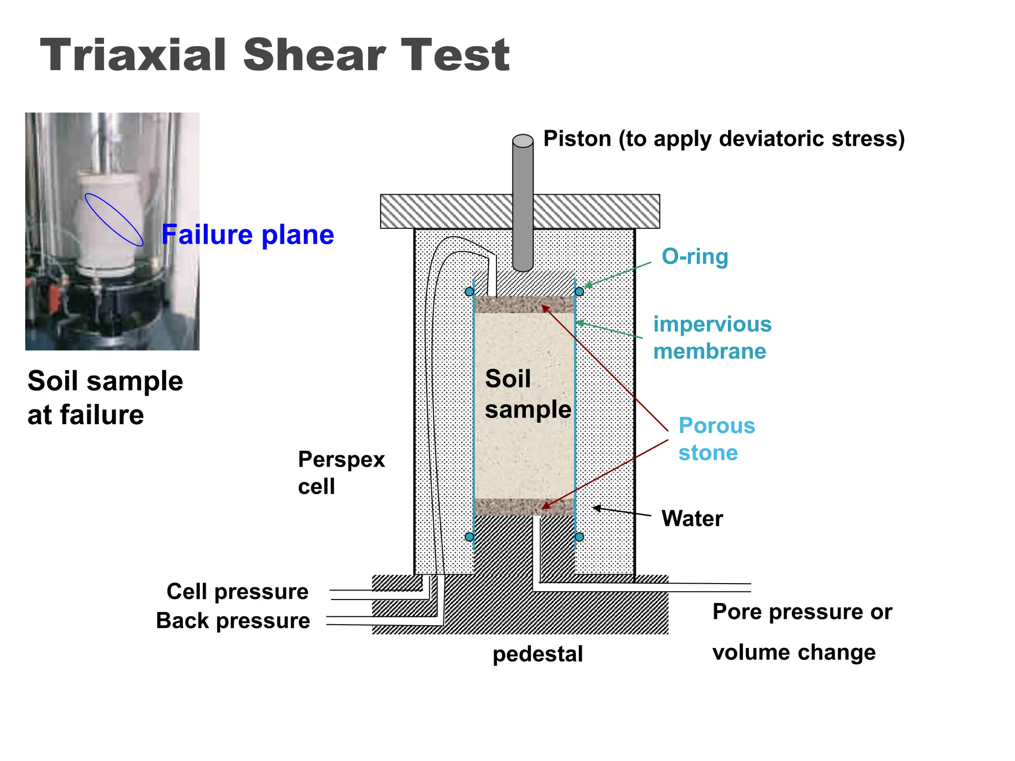
Triaxial Shear Test
Soilsample
at failure
Failure plane
Porous
stone
impervious
membrane
Piston (to apply deviatoric stress)
O-ring
pedestal
Perspex
cell
Cell pressure
Back pressure Pore pressure or
volume change
Water
Soil
sample
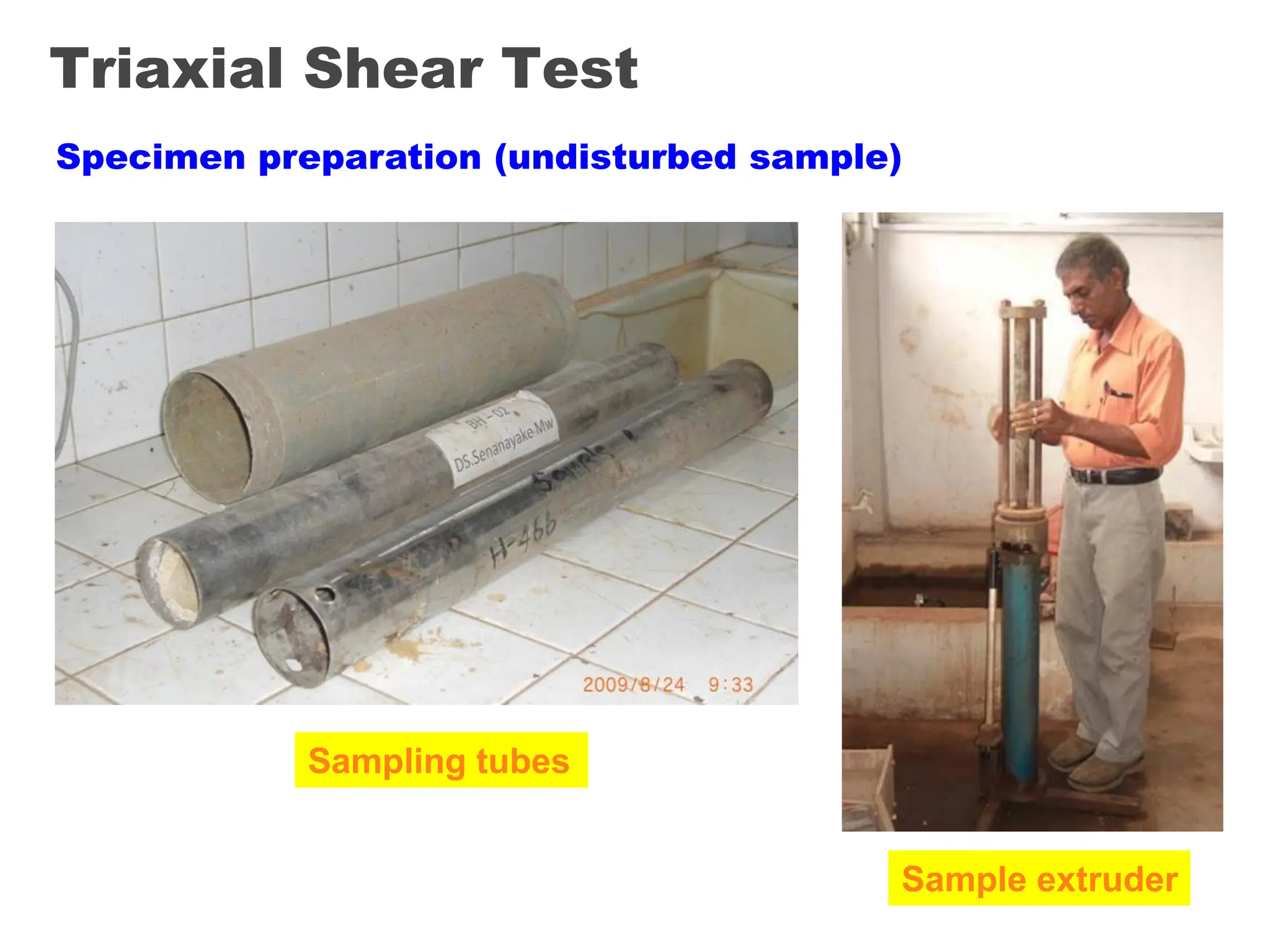
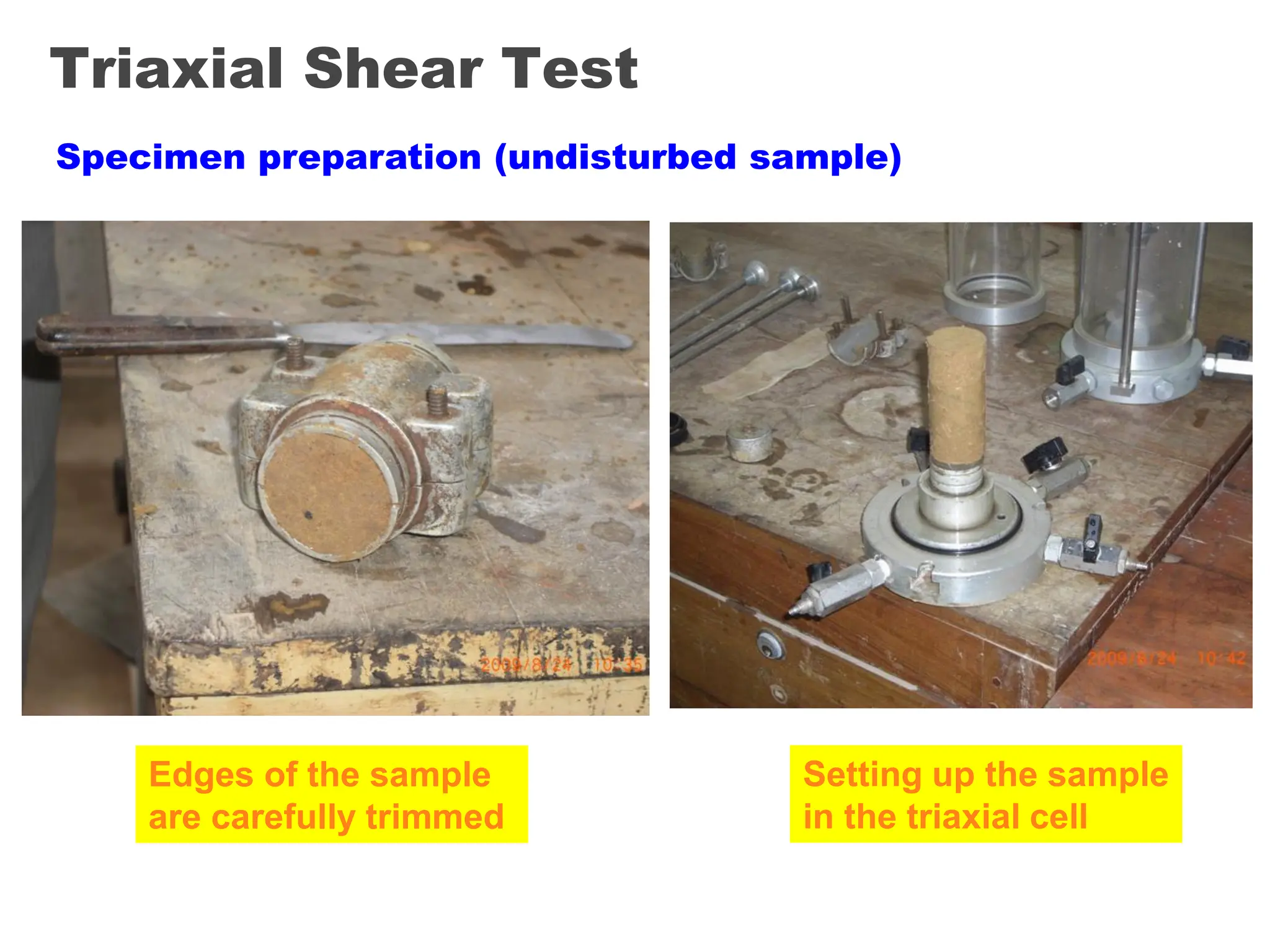
Triaxial Shear Test
Specimenpreparation (undisturbed sample)
Edges of the sample
are carefully trimmed
Setting up the sample
in the triaxial cell
44.
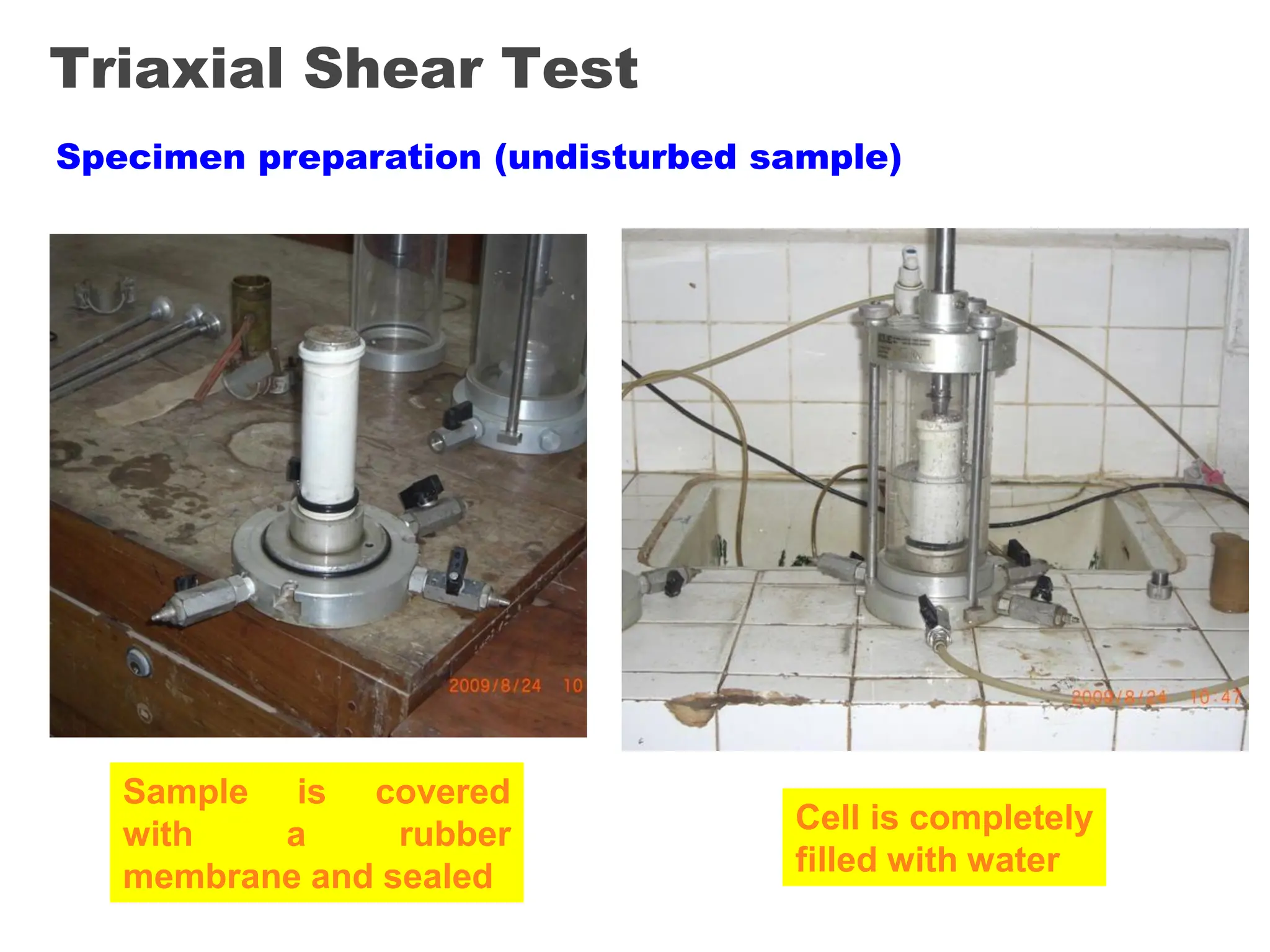
Triaxial Shear Test
Sampleis covered
with a rubber
membrane and sealed
Cell is completely
filled with water
Specimen preparation (undisturbed sample)
45.
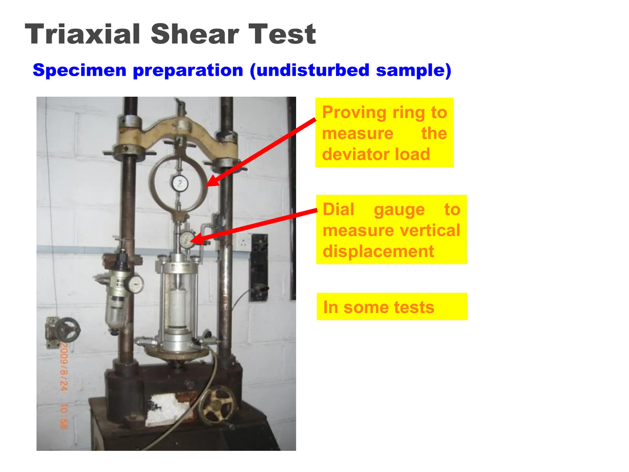
Triaxial Shear Test
Specimenpreparation (undisturbed sample)
Proving ring to
measure the
deviator load
Dial gauge to
measure vertical
displacement
In some tests
46.
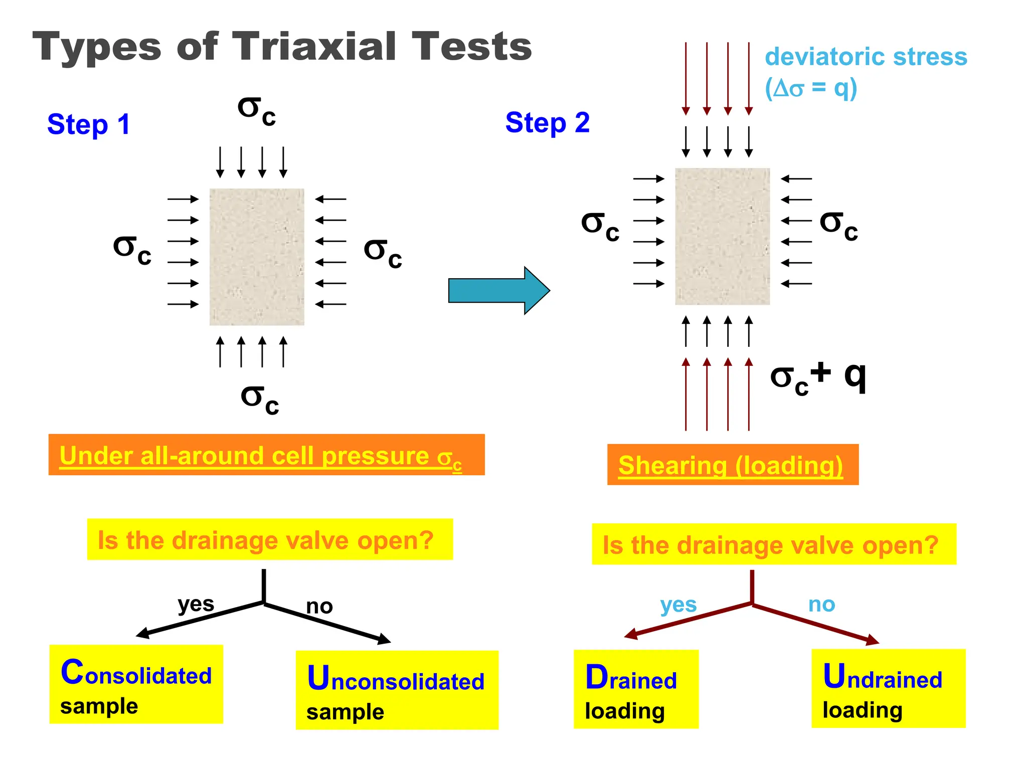
Types of TriaxialTests
Is the drainage valve open?
yes no
Consolidated
sample
Unconsolidated
sample
Is the drainage valve open?
yes no
Drained
loading
Undrained
loading
Under all-around cell pressure c
c
c
c
c
Step 1
deviatoric stress
( = q)
Shearing (loading)
Step 2
c c
c+ q
47.
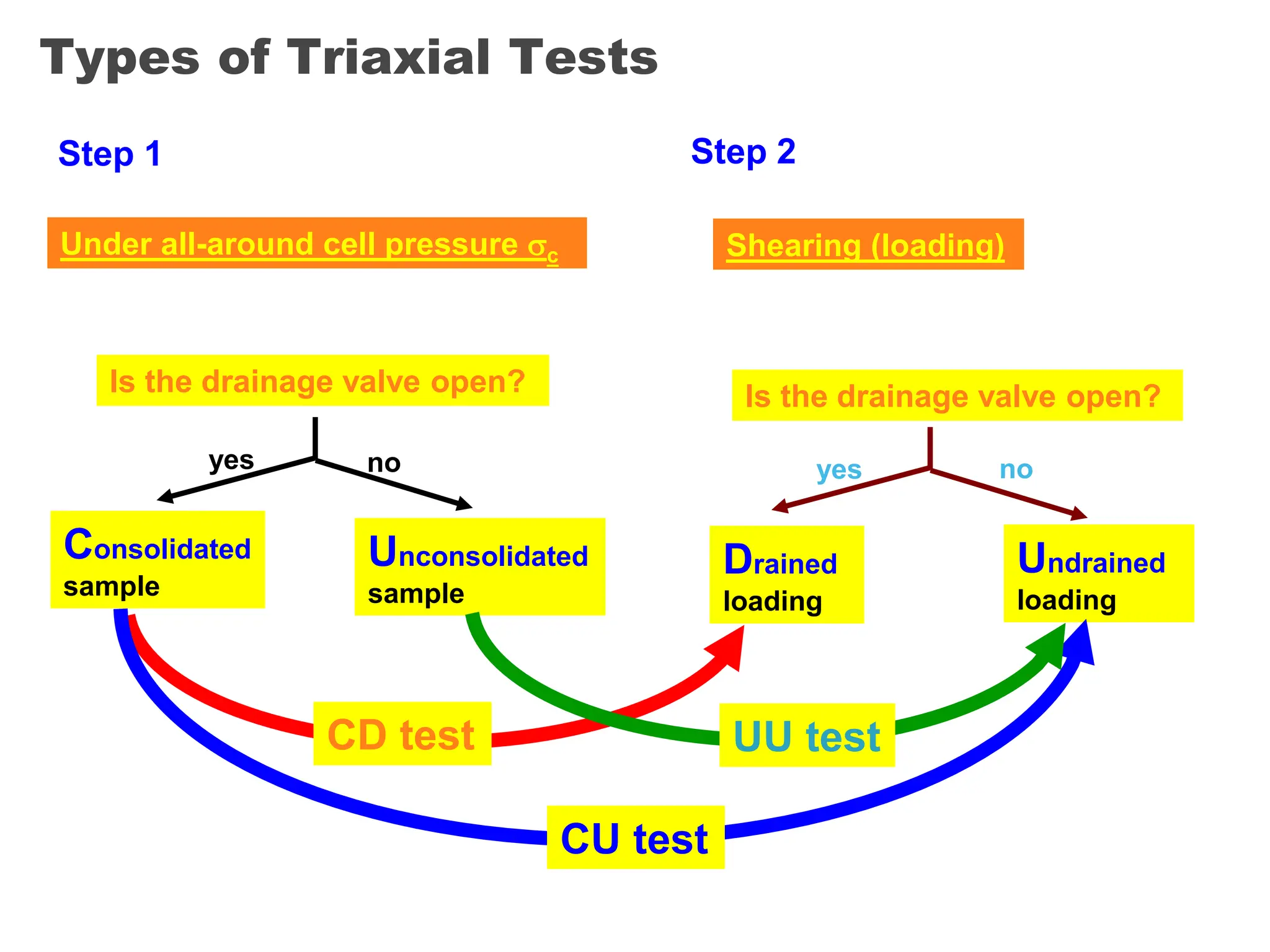
Types of TriaxialTests
Is the drainage valve open?
yes no
Consolidated
sample
Unconsolidated
sample
Under all-around cell pressure c
Step 1
Is the drainage valve open?
yes no
Drained
loading
Undrained
loading
Shearing (loading)
Step 2
CD test
CU test
UU test
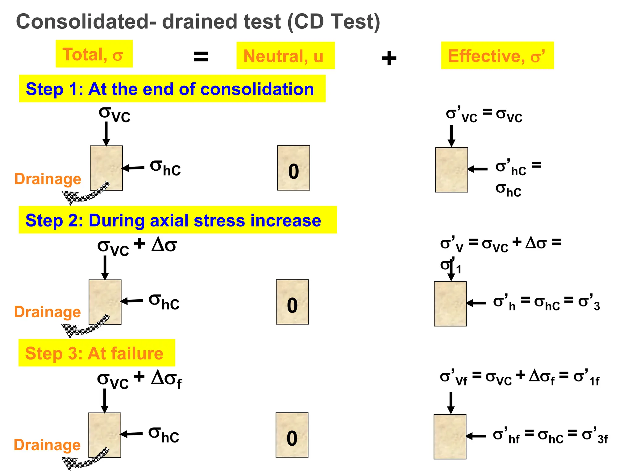
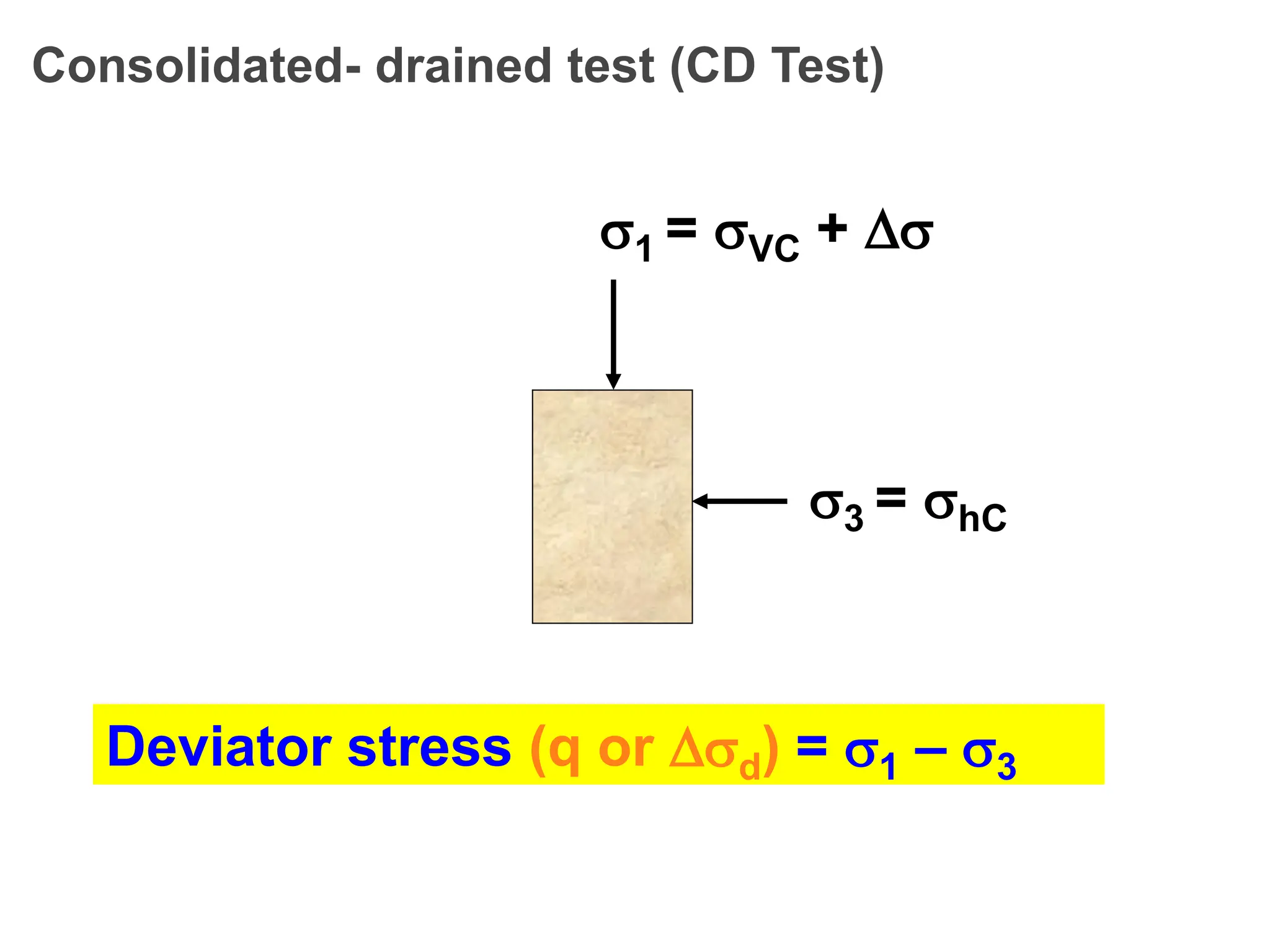
CD tests
Strength parametersc and obtained from CD tests
Since u = 0 in CD
tests, = ’
Therefore, c = c’
and = ’
cd and d are used
to denote them
54.
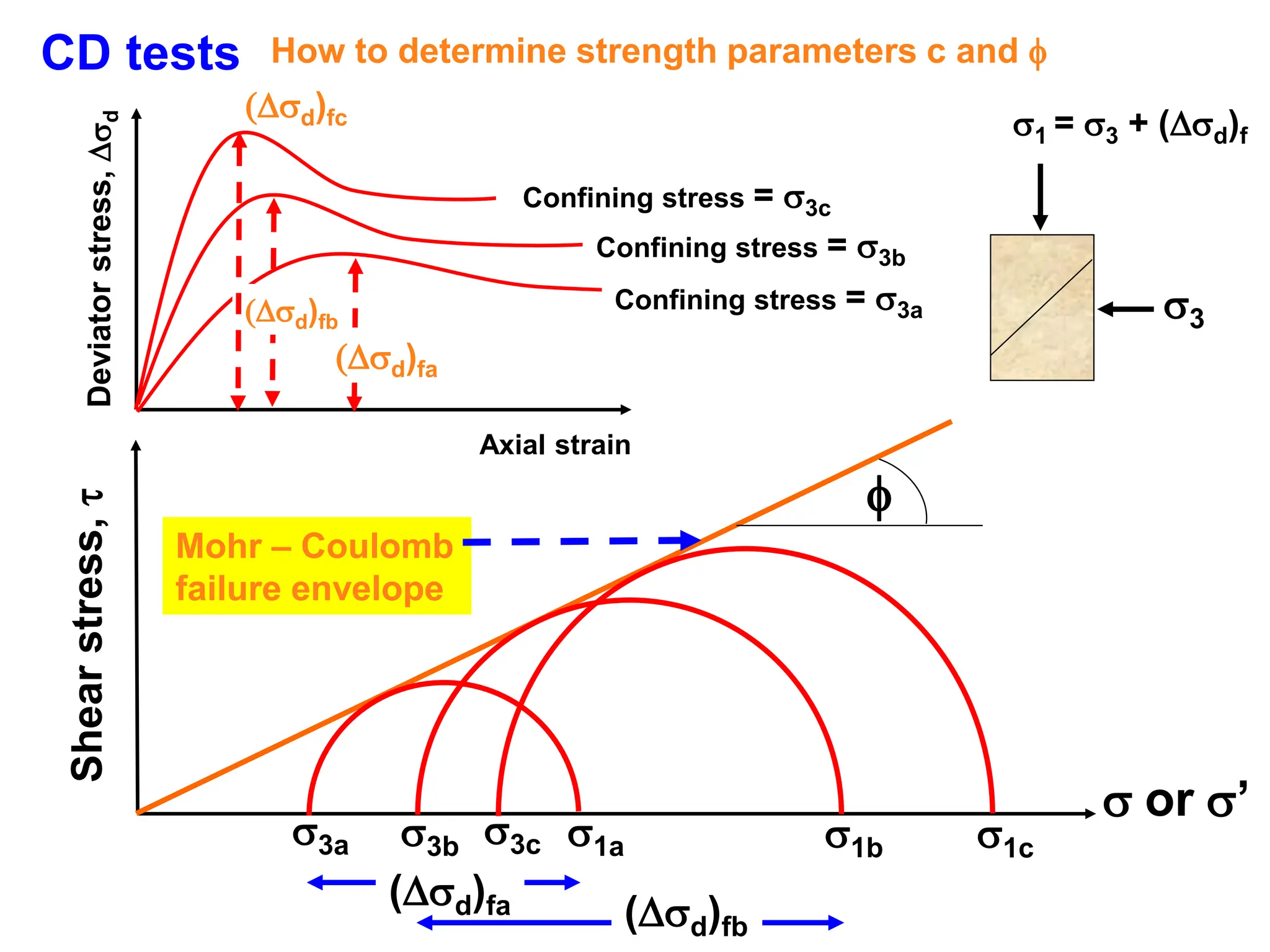
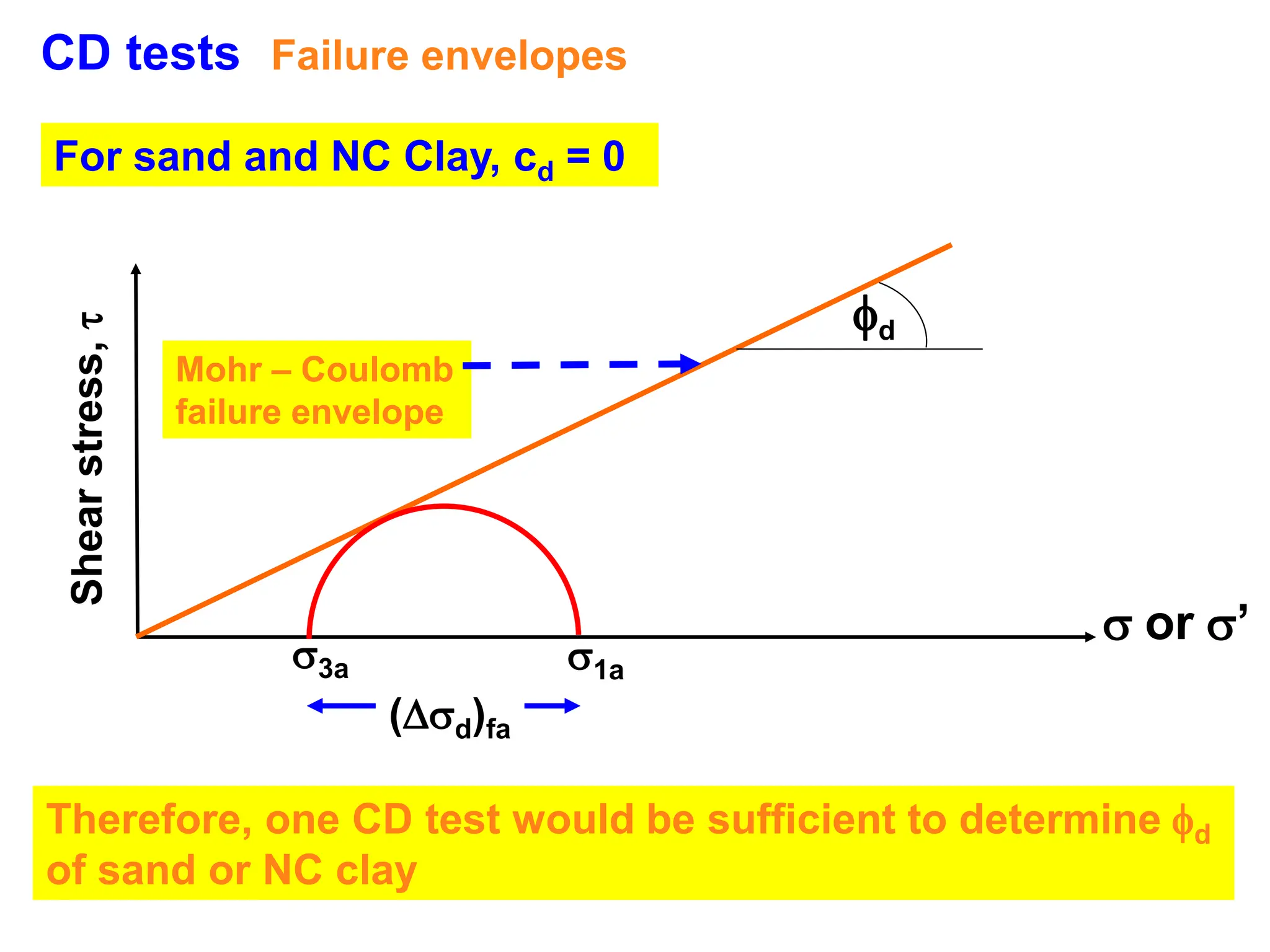
CD tests Failureenvelopes
Shear
stress,
or ’
d
Mohr – Coulomb
failure envelope
3a 1a
(d)fa
For sand and NC Clay, cd = 0
Therefore, one CD test would be sufficient to determine d
of sand or NC clay
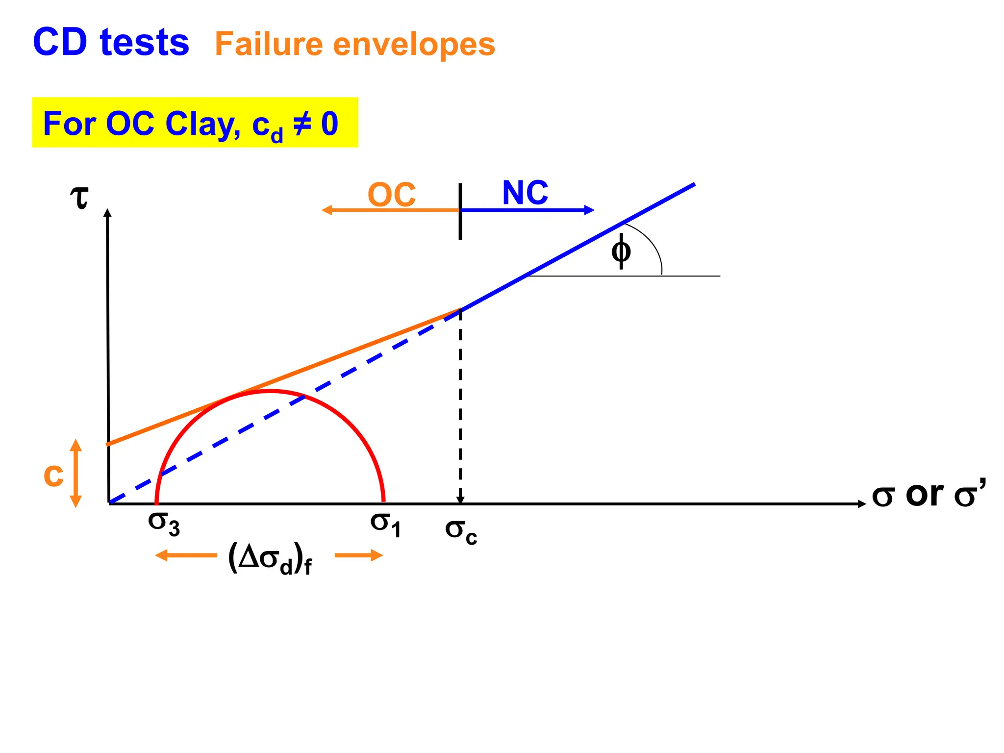
55.
CD tests Failureenvelopes
For OC Clay, cd ≠ 0
or ’
3 1
(d)f
c
c
OC NC
56.
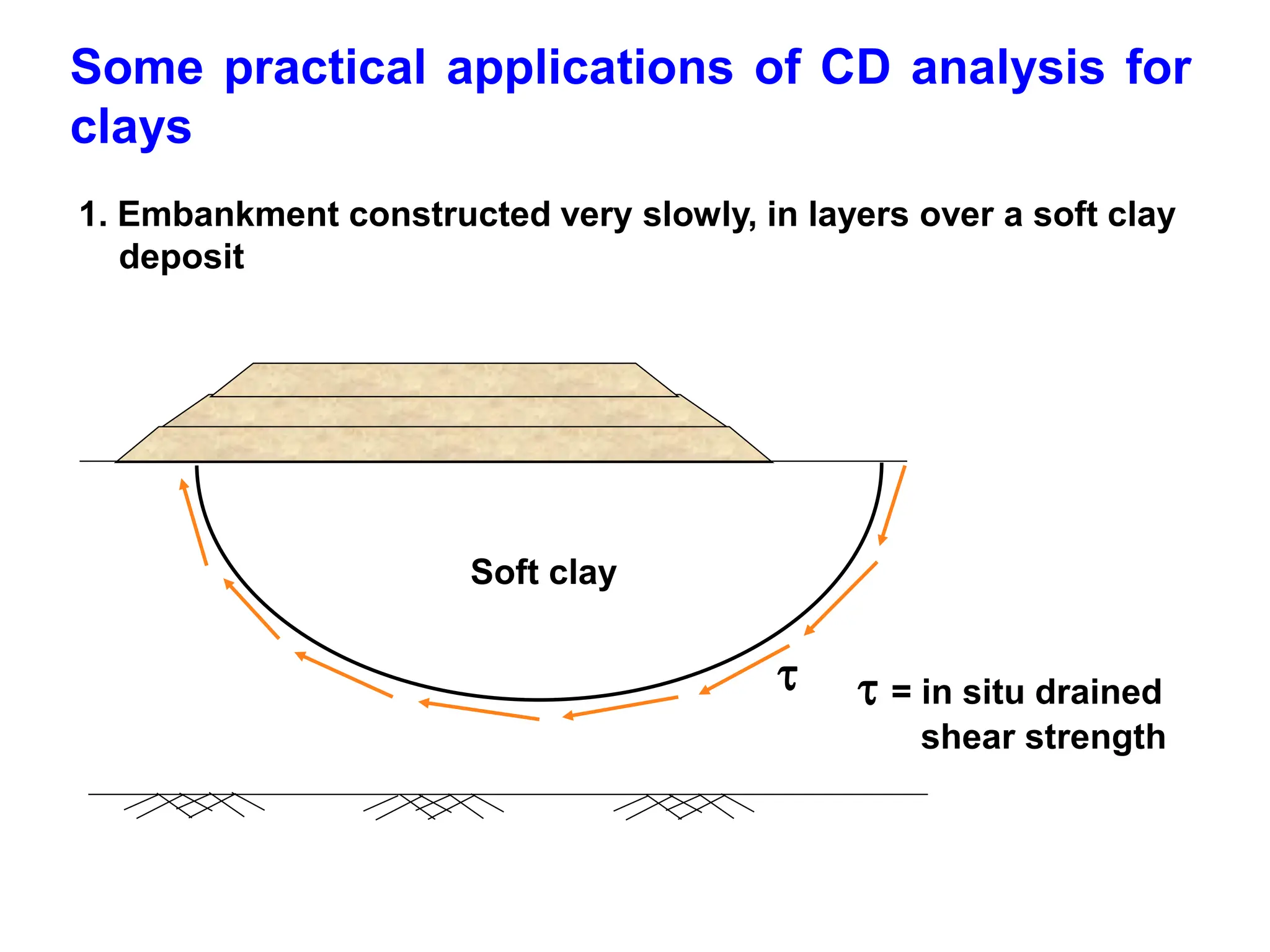
Some practical applicationsof CD analysis for
clays
= in situ drained
shear strength
Soft clay
1. Embankment constructed very slowly, in layers over a soft clay
deposit
57.
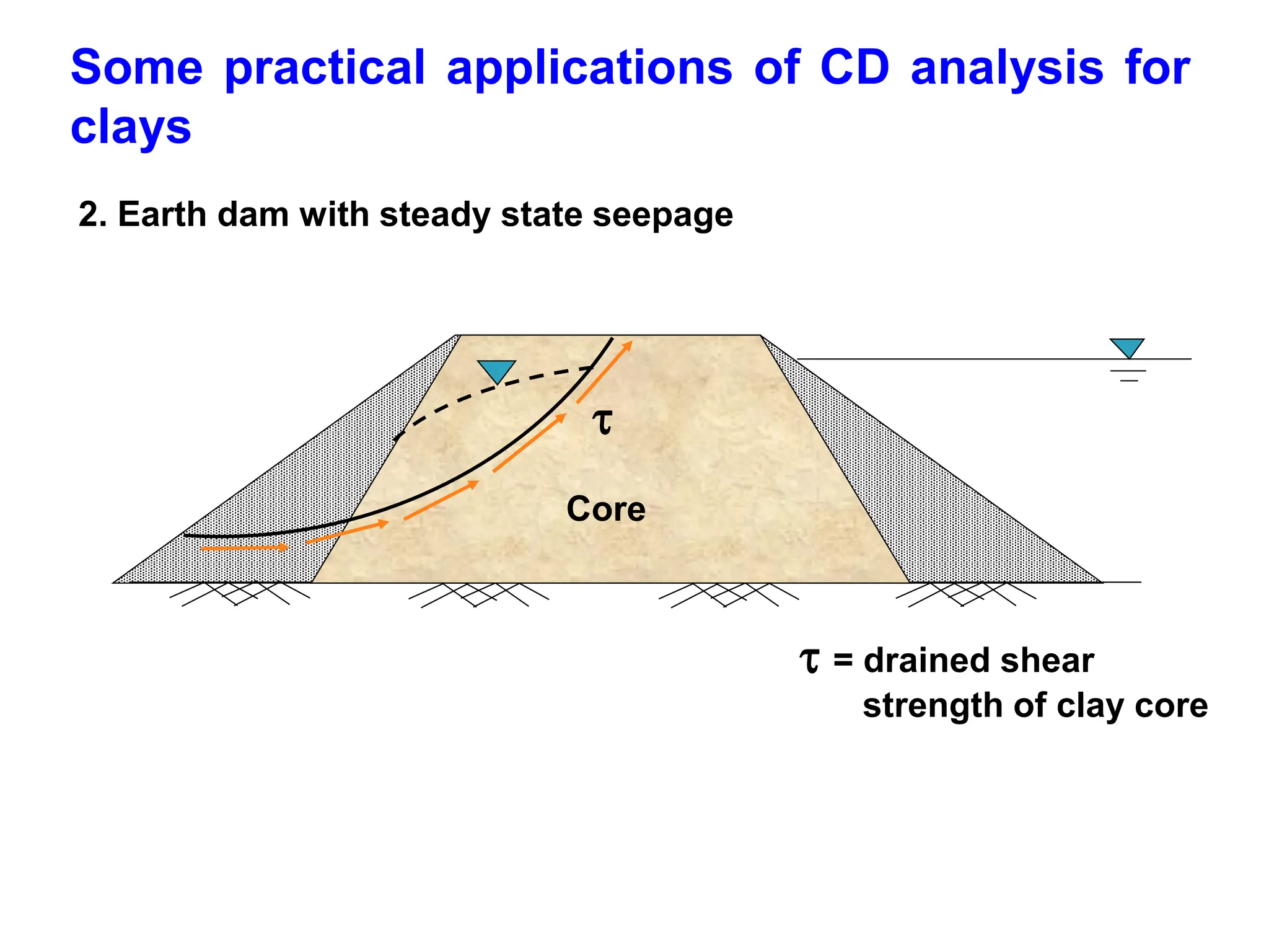
Some practical applicationsof CD analysis for
clays
2. Earth dam with steady state seepage
= drained shear
strength of clay core
Core
58.
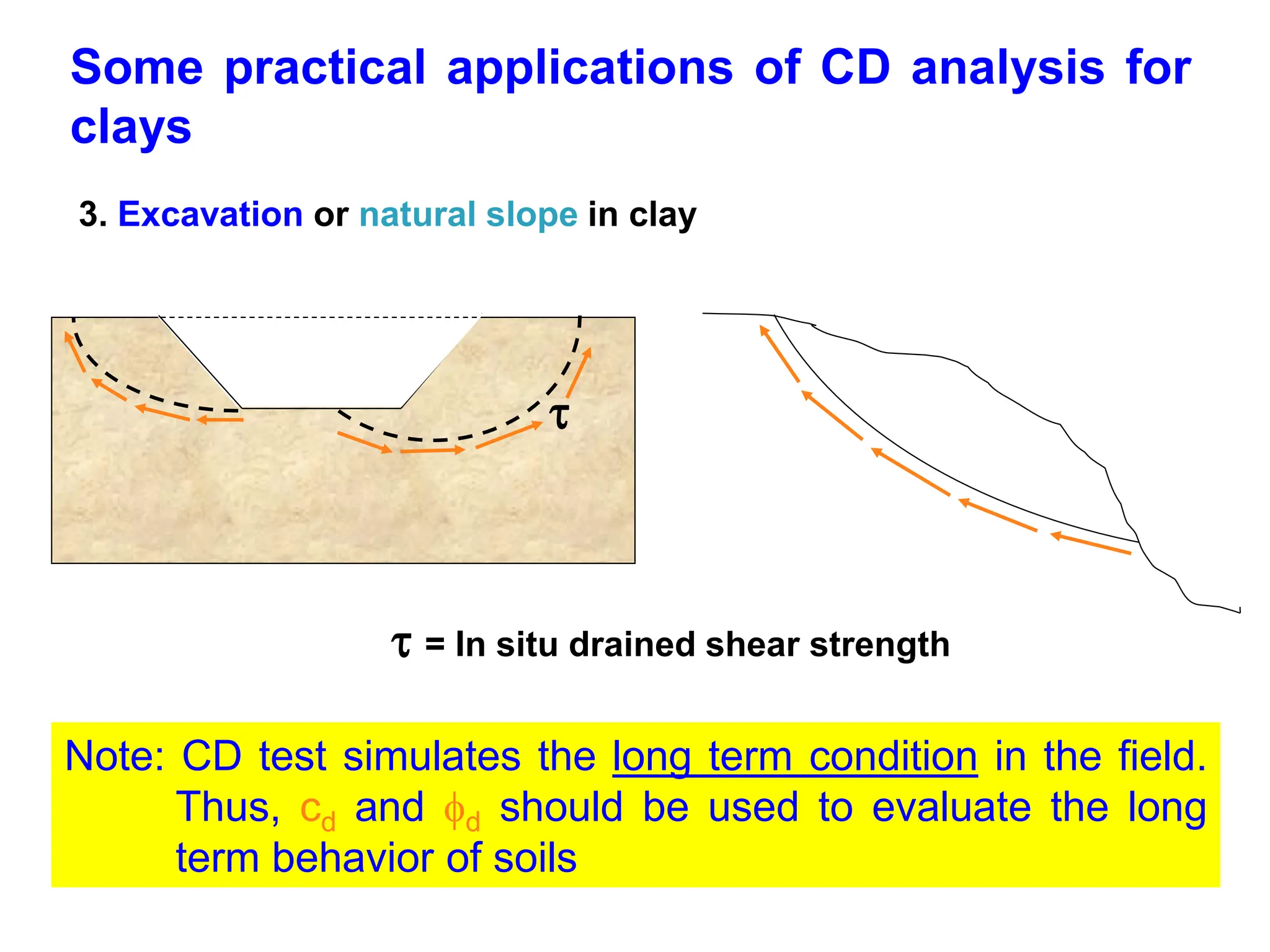
Some practical applicationsof CD analysis for
clays
3. Excavation or natural slope in clay
= In situ drained shear strength
Note: CD test simulates the long term condition in the field.
Thus, cd and d should be used to evaluate the long
term behavior of soils
59.
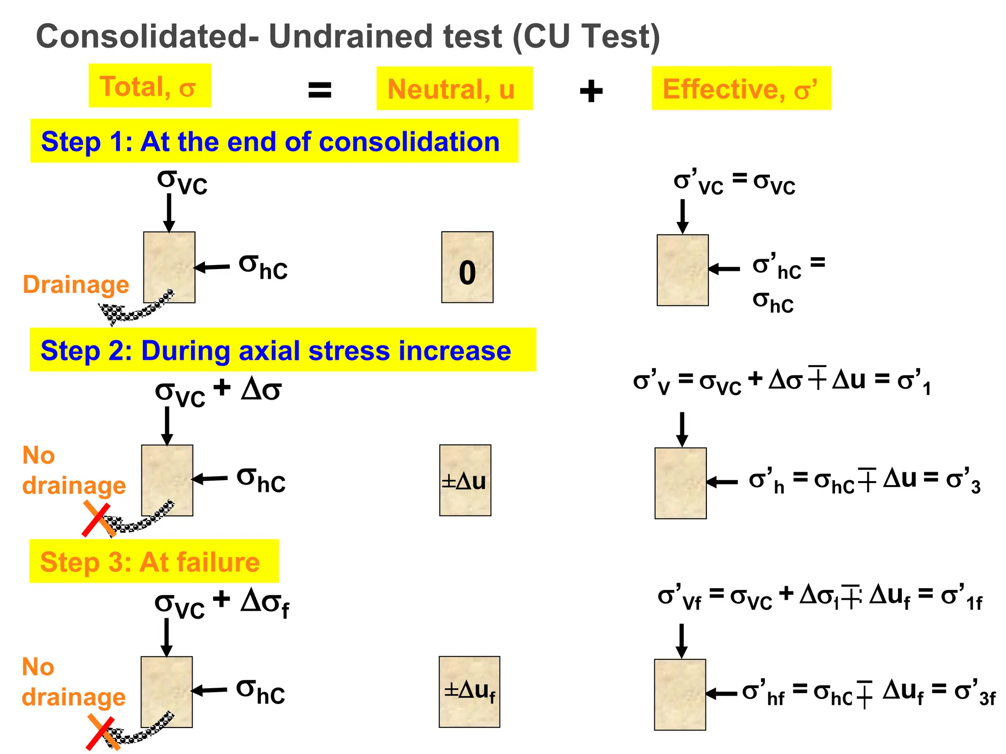
Consolidated- Undrained test(CU Test)
Step 1: At the end of consolidation
VC
hC
Total, = Neutral, u Effective, ’
+
0
Step 2: During axial stress increase
’VC = VC
’hC =
hC
VC +
hC ±u
Drainage
Step 3: At failure
VC + f
hC
No
drainage
No
drainage ±uf
’V = VC + ± u = ’1
’h = hC ± u = ’3
’Vf = VC + f ± uf = ’1f
’hf = hC ± uf = ’3f
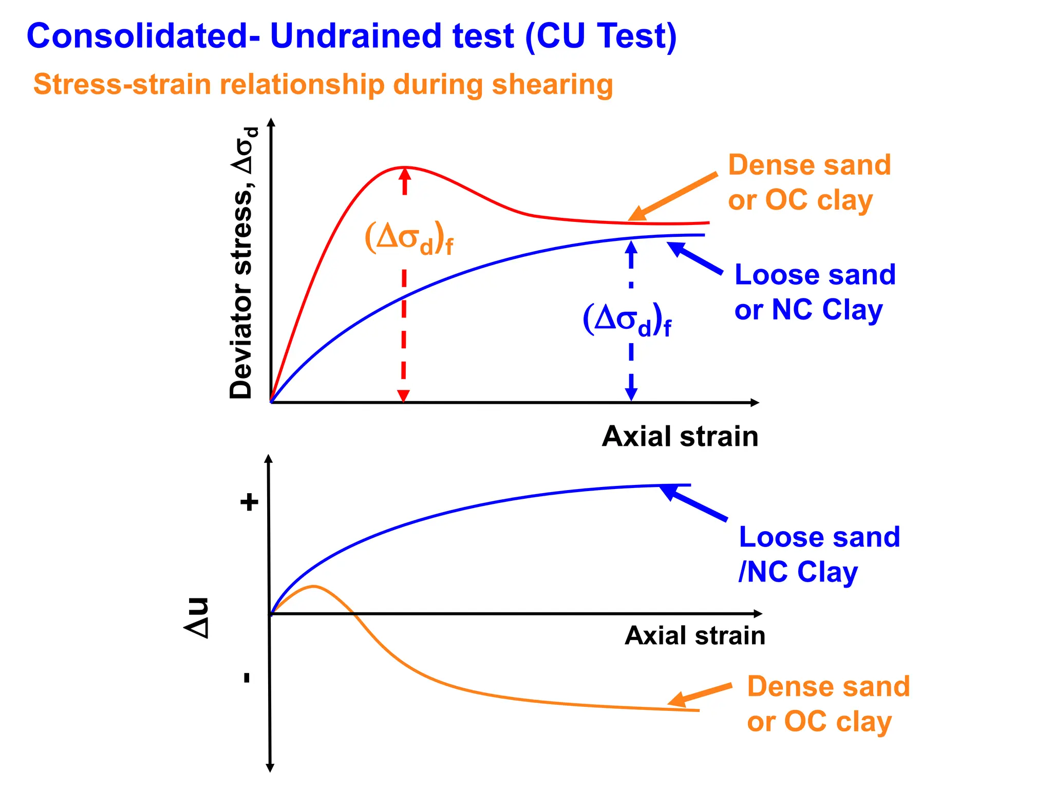
Deviator
stress,
d
Axial strain
Dense sand
orOC clay
(d)f
Dense sand
or OC clay
Loose sand
/NC Clay
u
+
-
Axial strain
Stress-strain relationship during shearing
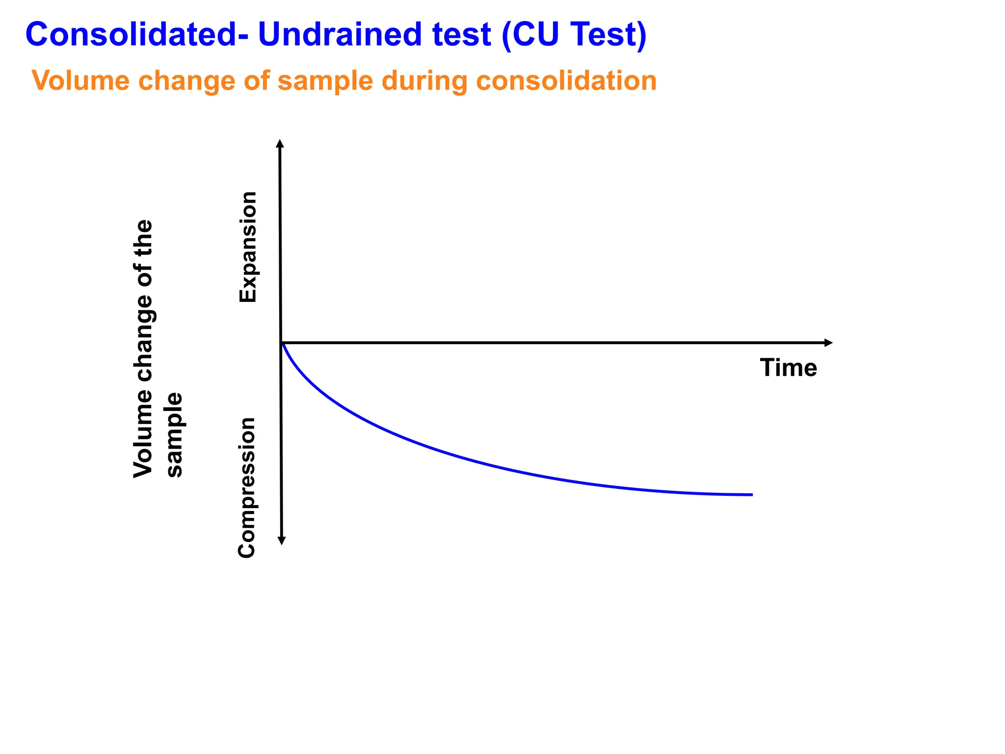
Consolidated- Undrained test (CU Test)
Loose sand
or NC Clay
(d)f
62.
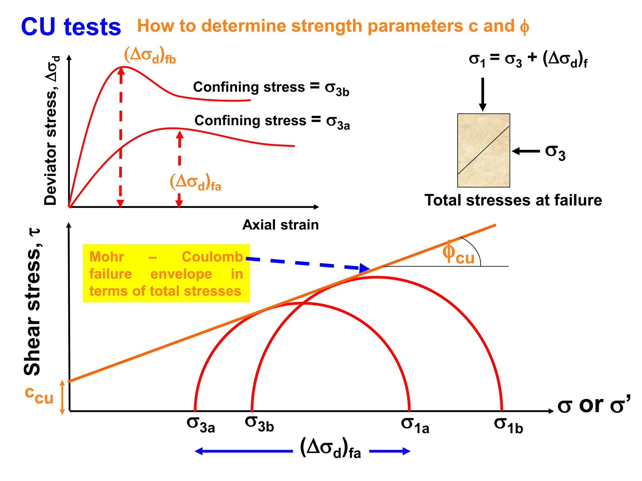
CU tests Howto determine strength parameters c and
Deviator
stress,
d
Axial strain
Shear
stress,
or ’
(d)fb
Confining stress = 3b
3b 1b
3a 1a
(d)fa
cu
Mohr – Coulomb
failure envelope in
terms of total stresses
ccu
1 = 3 + (d)f
3
Total stresses at failure
(d)fa
Confining stress = 3a
63.
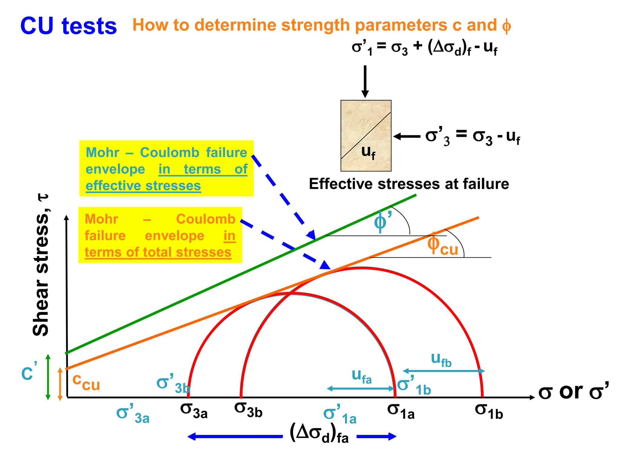
(d)fa
CU tests Howto determine strength parameters c and
Shear
stress,
or ’
3b 1b
3a 1a
(d)fa
cu
Mohr – Coulomb
failure envelope in
terms of total stresses
ccu ’3b ’1b
’3a ’1a
Mohr – Coulomb failure
envelope in terms of
effective stresses
’
C’ ufa
ufb
’1 = 3 + (d)f - uf
’3 = 3 - uf
Effective stresses at failure
uf
64.
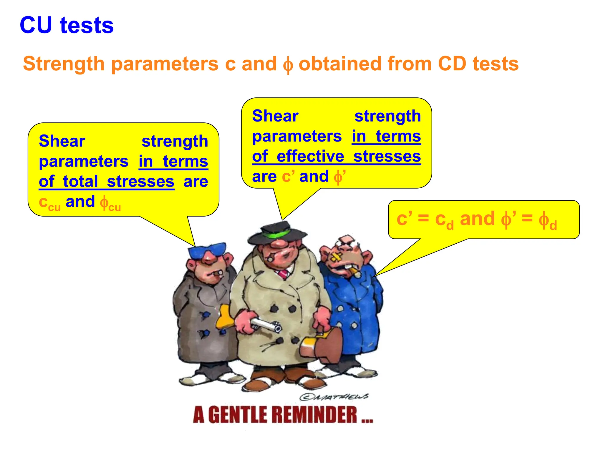
CU tests
Strength parametersc and obtained from CD tests
Shear strength
parameters in terms
of total stresses are
ccu and cu
Shear strength
parameters in terms
of effective stresses
are c’ and ’
c’ = cd and ’ = d
65.
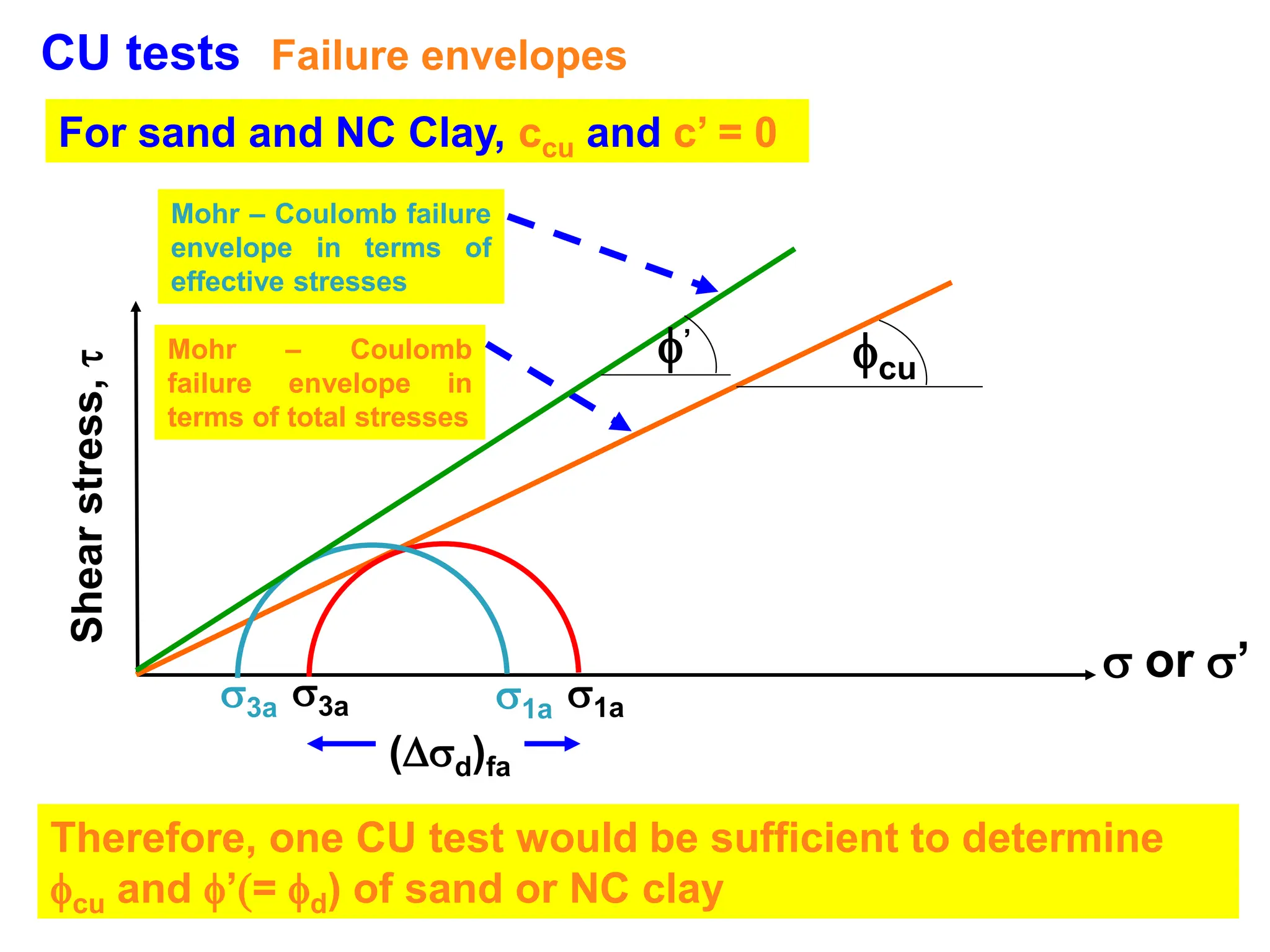
CU tests Failureenvelopes
For sand and NC Clay, ccu and c’ = 0
Therefore, one CU test would be sufficient to determine
cu and ’(= d) of sand or NC clay
Shear
stress,
or ’
cu
Mohr – Coulomb
failure envelope in
terms of total stresses
3a 1a
(d)fa
3a 1a
’
Mohr – Coulomb failure
envelope in terms of
effective stresses
66.
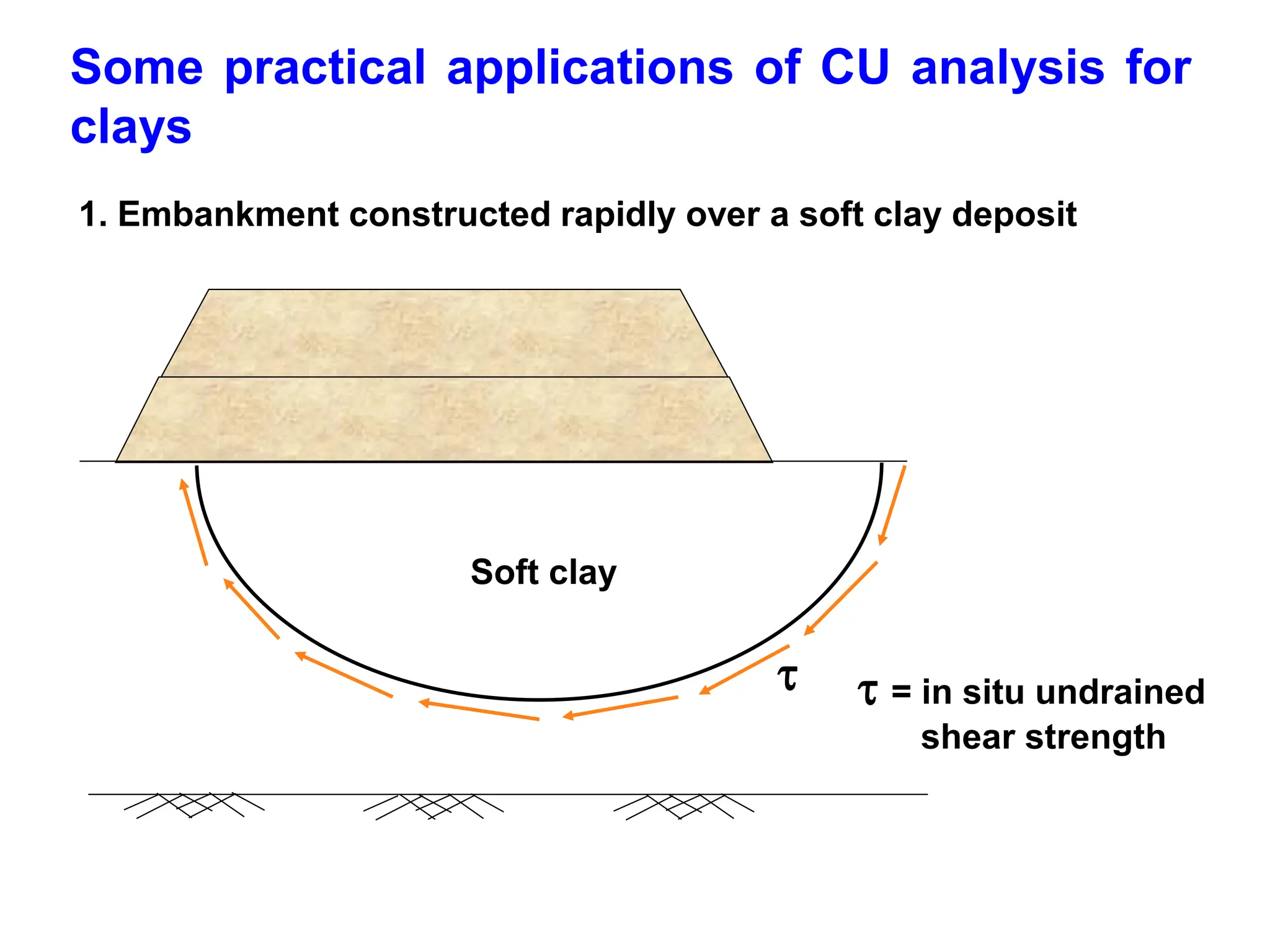
Some practical applicationsof CU analysis for
clays
= in situ undrained
shear strength
Soft clay
1. Embankment constructed rapidly over a soft clay deposit
67.
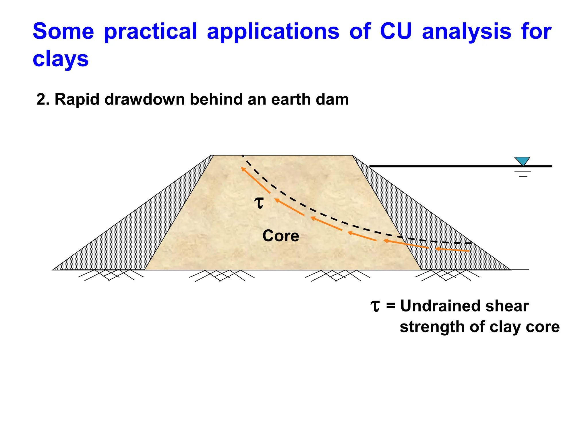
Some practical applicationsof CU analysis for
clays
2. Rapid drawdown behind an earth dam
= Undrained shear
strength of clay core
Core
68.
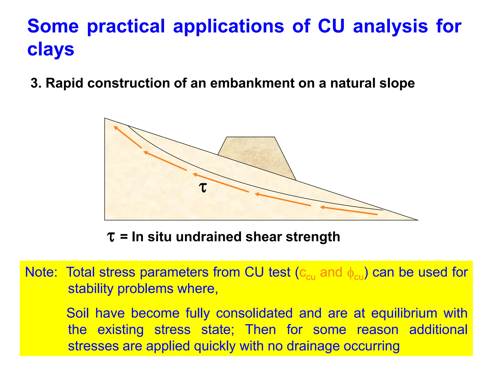
Some practical applicationsof CU analysis for
clays
3. Rapid construction of an embankment on a natural slope
Note: Total stress parameters from CU test (ccu and cu) can be used for
stability problems where,
Soil have become fully consolidated and are at equilibrium with
the existing stress state; Then for some reason additional
stresses are applied quickly with no drainage occurring
= In situ undrained shear strength
70.
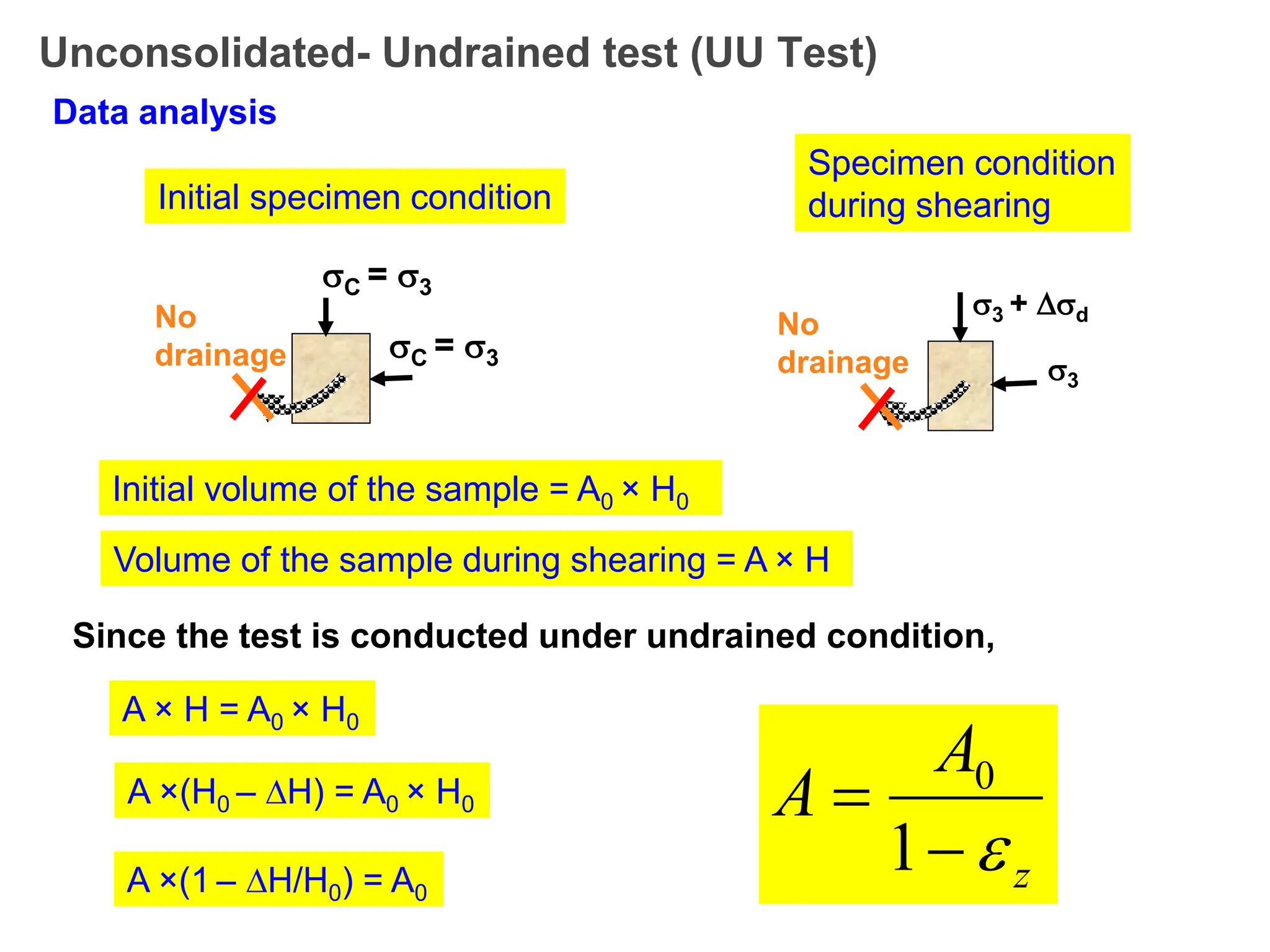
Unconsolidated- Undrained test(UU Test)
Data analysis
C = 3
C = 3
No
drainage
Initial specimen condition
3 + d
3
No
drainage
Specimen condition
during shearing
Initial volume of the sample = A0 × H0
Volume of the sample during shearing = A × H
Since the test is conducted under undrained condition,
A × H = A0 × H0
A ×(H0 – H) = A0 × H0
A ×(1 – H/H0) = A0
z
A
A
1
0
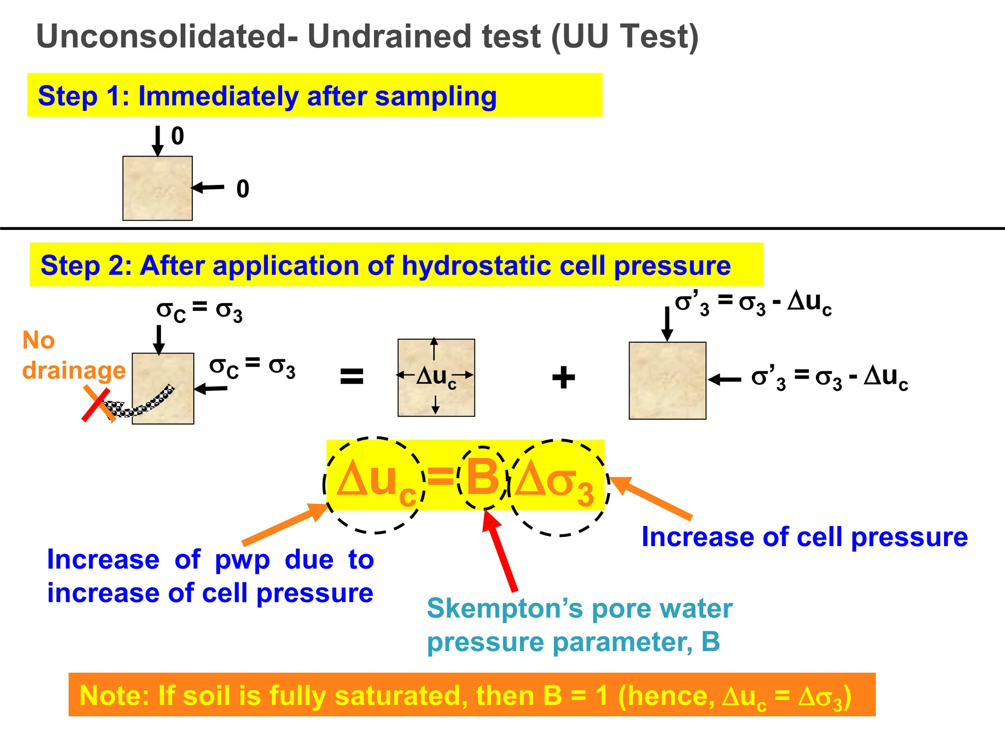
71.
Unconsolidated- Undrained test(UU Test)
Step 1: Immediately after sampling
0
0
= +
Step 2: After application of hydrostatic cell pressure
uc = B 3
C = 3
C = 3 uc
’3 = 3 - uc
’3 = 3 - uc
No
drainage
Increase of pwp due to
increase of cell pressure
Increase of cell pressure
Skempton’s pore water
pressure parameter, B
Note: If soil is fully saturated, then B = 1 (hence, uc = 3)
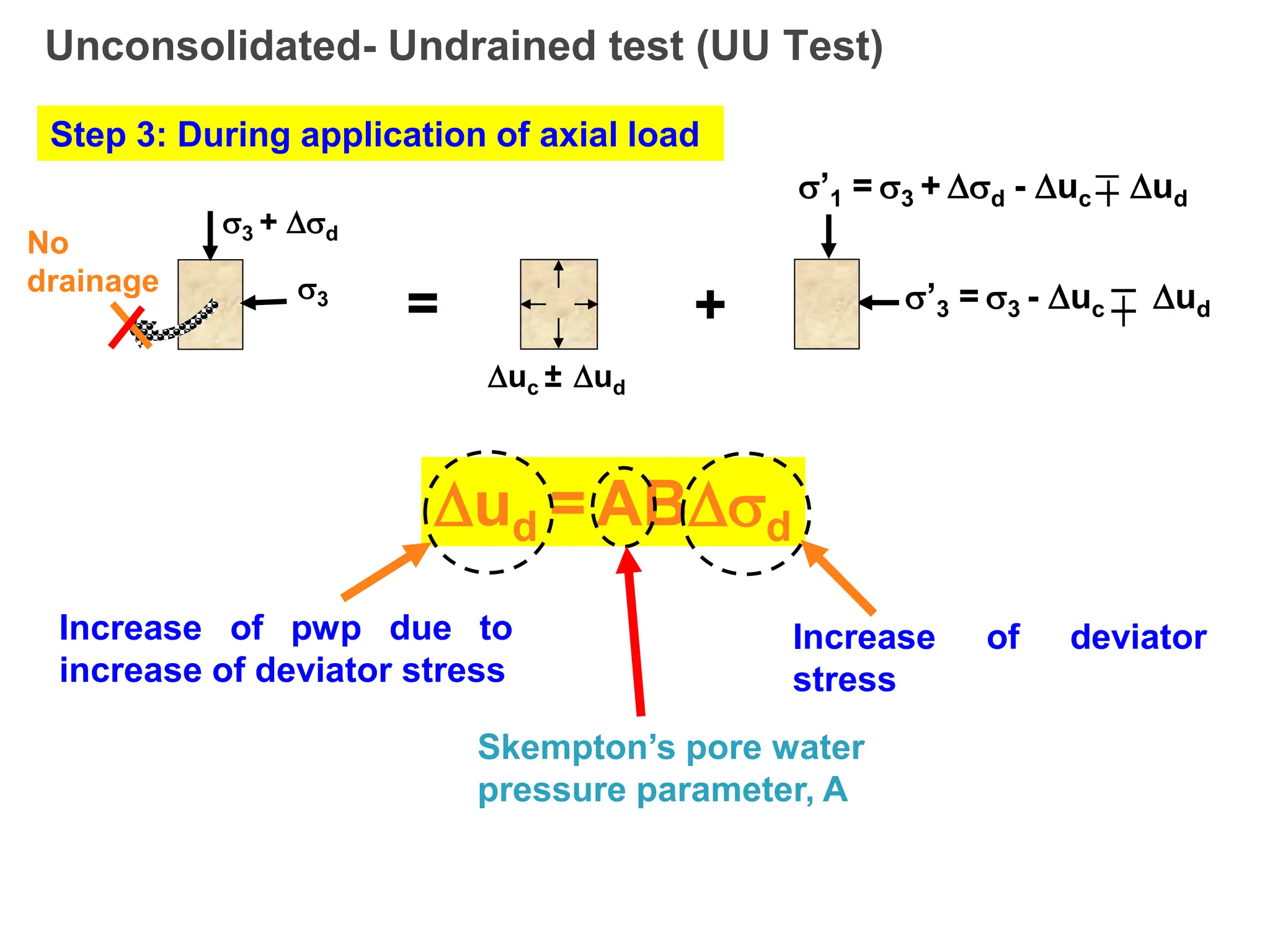
72.
Unconsolidated- Undrained test(UU Test)
Step 3: During application of axial load
3 + d
3
No
drainage
’1 = 3 + d - uc ud
’3 = 3 - uc ud
ud = ABd
uc ± ud
= +
Increase of pwp due to
increase of deviator stress
Increase of deviator
stress
Skempton’s pore water
pressure parameter, A
73.
Unconsolidated- Undrained test(UU Test)
Combining steps 2 and 3,
uc = B 3 ud = ABd
u = uc + ud
Total pore water pressure increment at any stage, u
u = B [3 + Ad]
Skempton’s pore
water pressure
equation
u = B [3 + A(1 – 3]
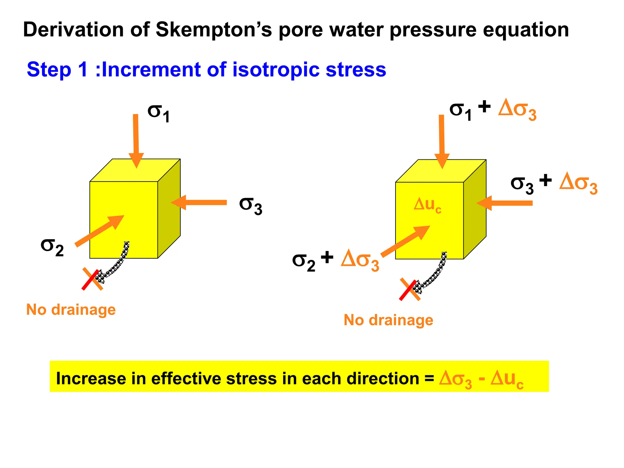
Step 1 :Incrementof isotropic stress
Derivation of Skempton’s pore water pressure equation
2
3
1
No drainage
1 + 3
3 + 3
2 + 3
No drainage
uc
Increase in effective stress in each direction = 3 - uc
76.
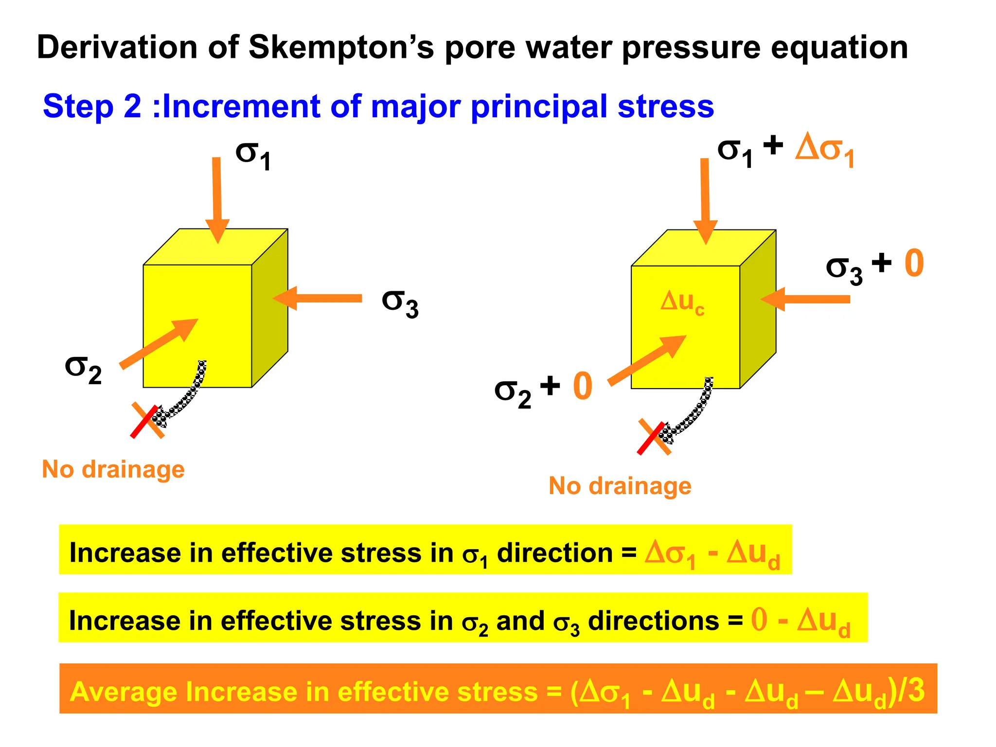
Step 2 :Incrementof major principal stress
Derivation of Skempton’s pore water pressure equation
2
3
1
No drainage
1 + 1
3 + 0
2 + 0
No drainage
uc
Increase in effective stress in 1 direction = 1 - ud
Increase in effective stress in 2 and 3 directions = 0 - ud
Average Increase in effective stress = (1 - ud - ud – ud)/3
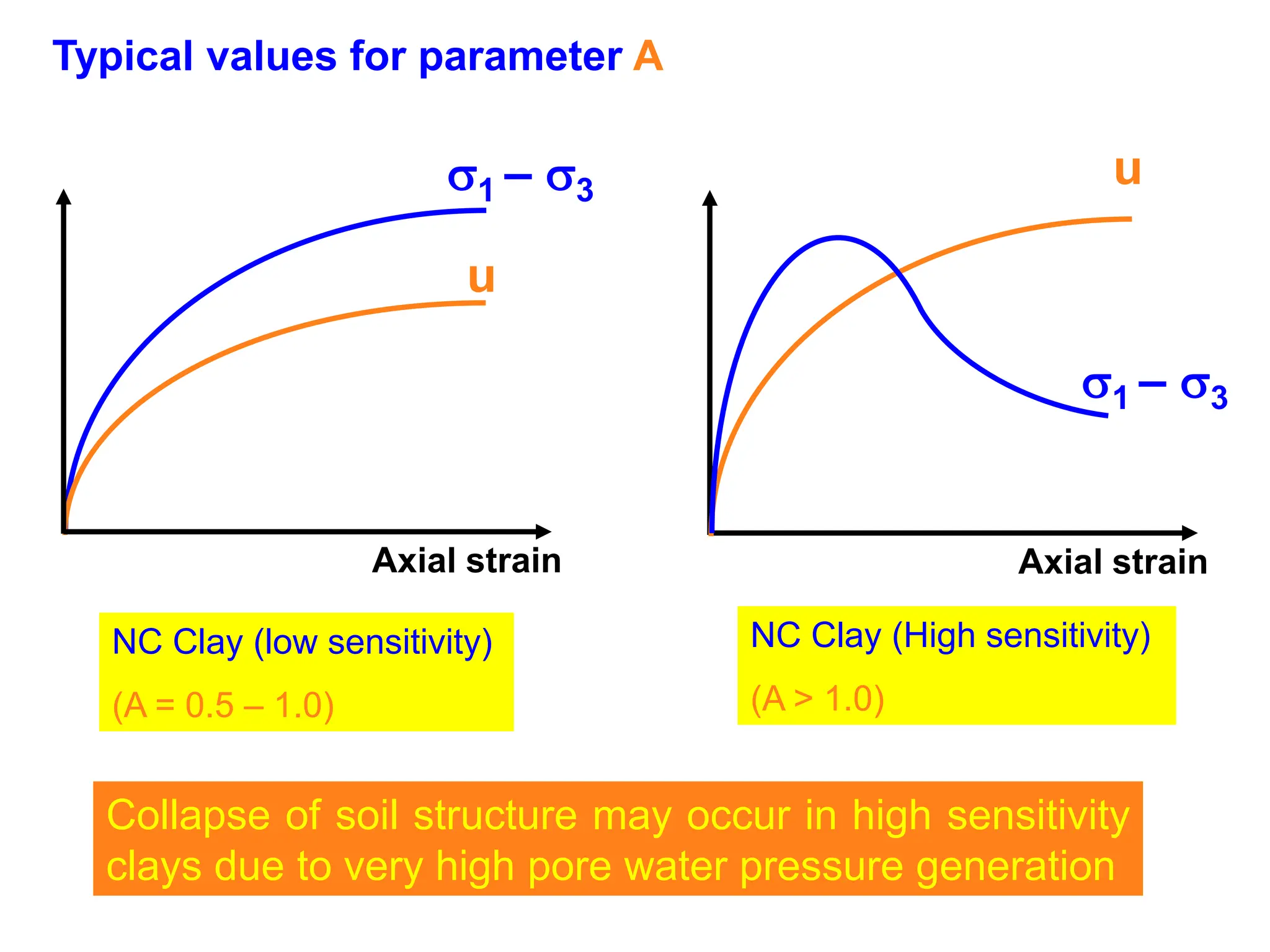
Typical values forparameter A
1 – 3
u
Axial strain
NC Clay (low sensitivity)
(A = 0.5 – 1.0)
NC Clay (High sensitivity)
(A > 1.0)
Axial strain
u
1 – 3
Collapse of soil structure may occur in high sensitivity
clays due to very high pore water pressure generation
79.
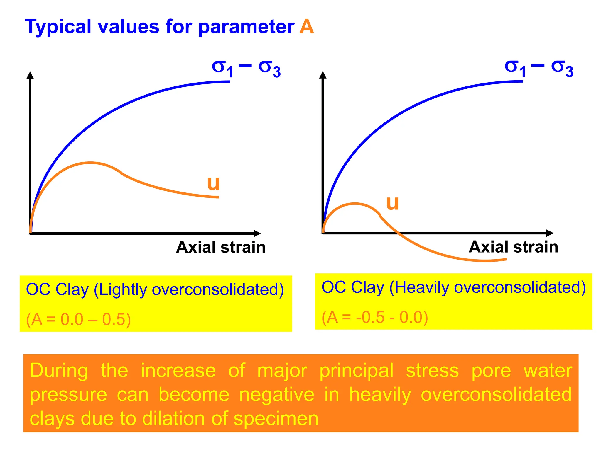
Typical values forparameter A
1 – 3
Axial strain
OC Clay (Lightly overconsolidated)
(A = 0.0 – 0.5)
OC Clay (Heavily overconsolidated)
(A = -0.5 - 0.0)
During the increase of major principal stress pore water
pressure can become negative in heavily overconsolidated
clays due to dilation of specimen
u
1 – 3
Axial strain
u
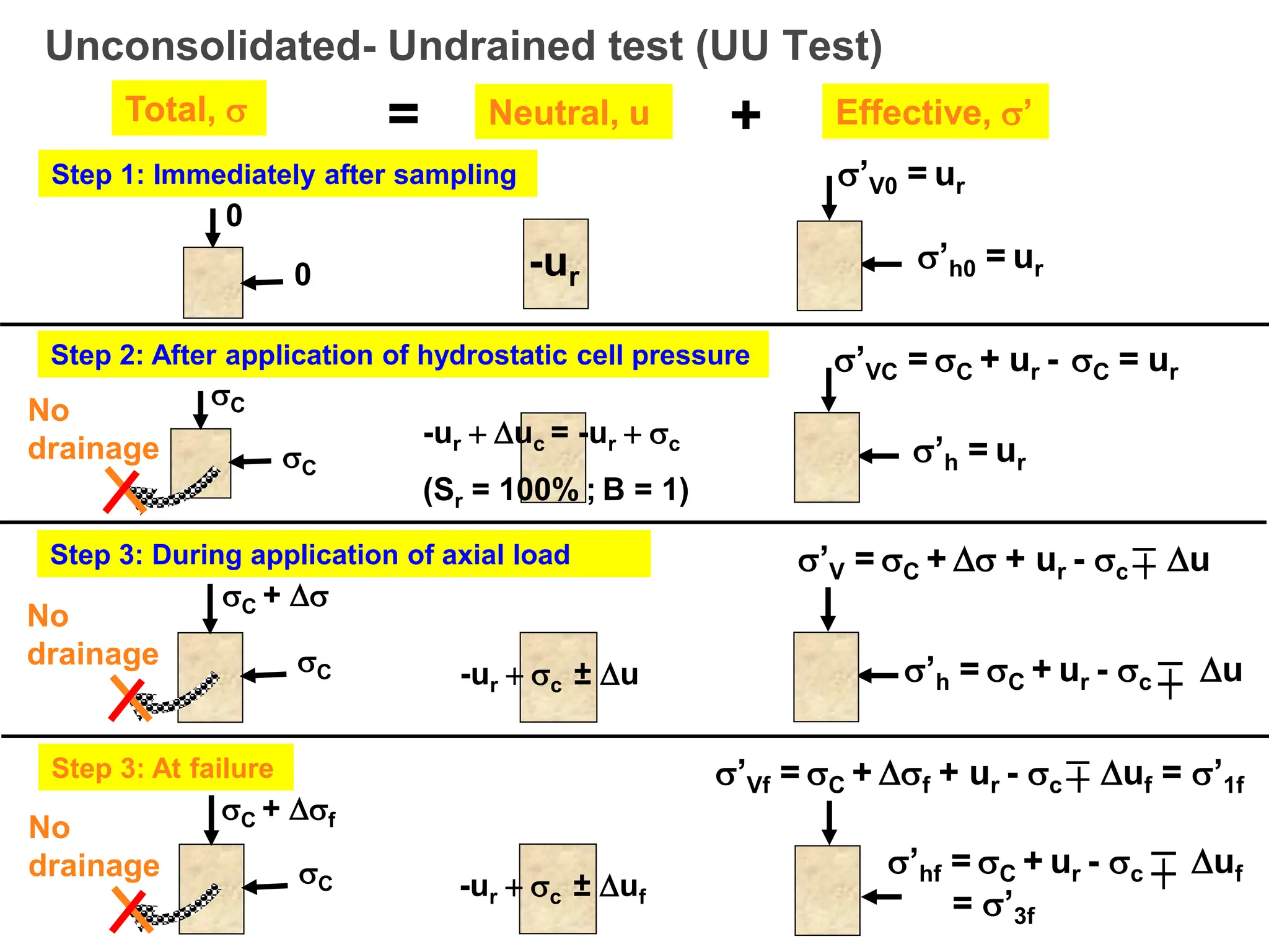
Unconsolidated- Undrained test(UU Test)
Step 1: Immediately after sampling
0
0
Total, = Neutral, u Effective, ’
+
-ur
Step 2: After application of hydrostatic cell pressure
’V0 = ur
’h0 = ur
C
C
-ur uc = -ur c
(Sr = 100% ; B = 1)
Step 3: During application of axial load
C +
C
No
drainage
No
drainage
-ur c ± u
’VC = C + ur - C = ur
’h = ur
Step 3: At failure
’V = C + + ur - c u
’h = C + ur - c u
’hf = C + ur - c uf
= ’3f
’Vf = C + f + ur - c uf = ’1f
-ur c ± uf
C
C + f
No
drainage
82.
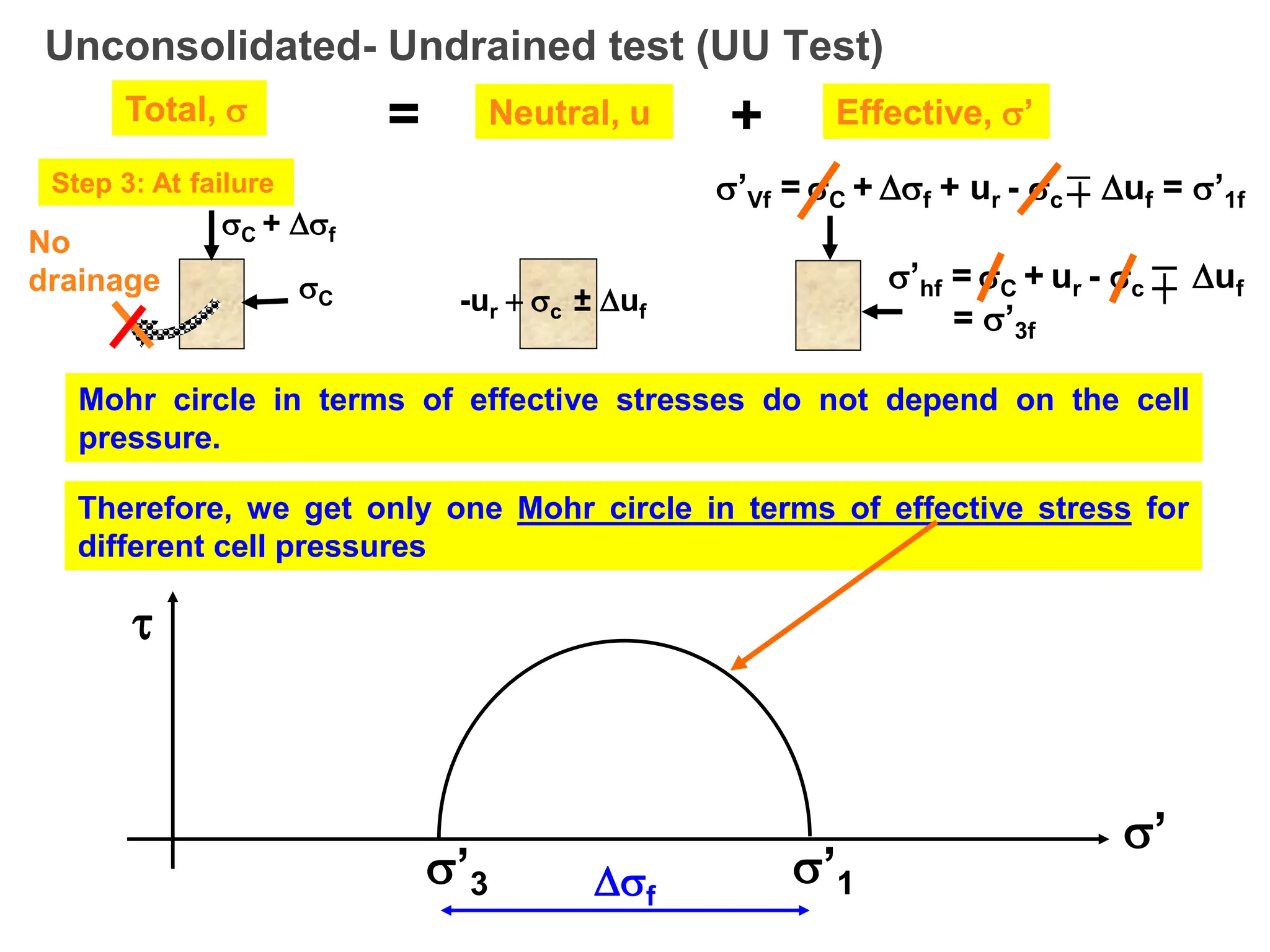
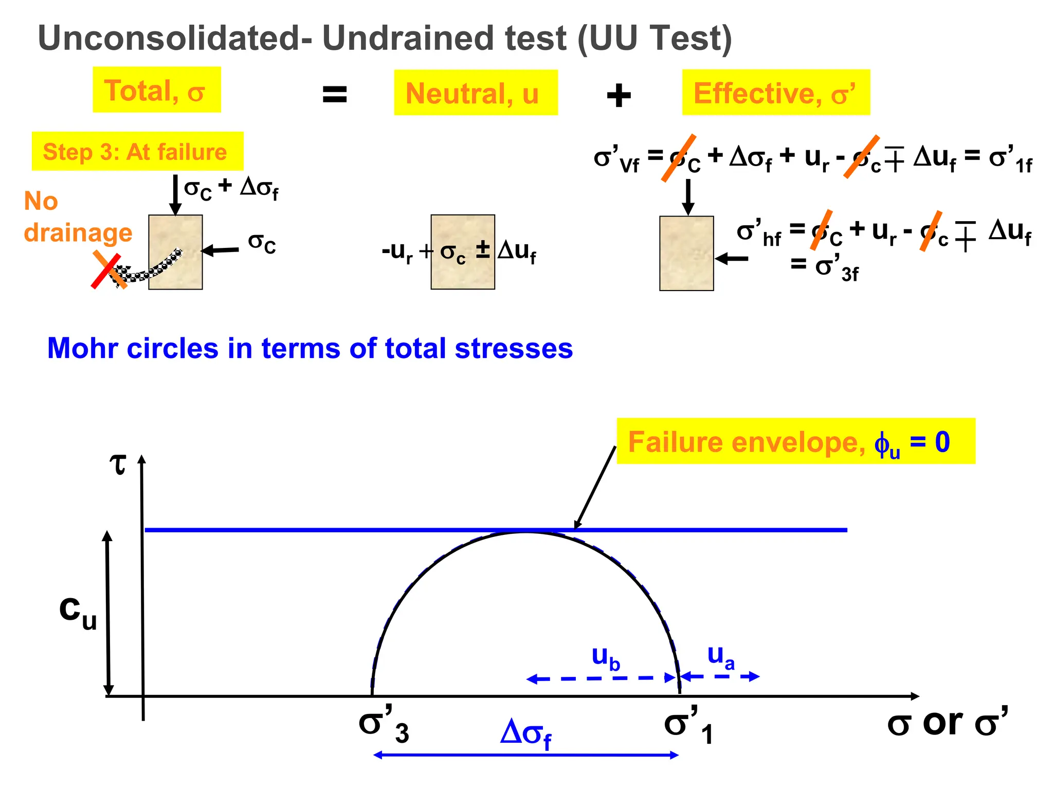
Unconsolidated- Undrained test(UU Test)
Total, = Neutral, u Effective, ’
+
Step 3: At failure
’hf = C + ur - c uf
= ’3f
’Vf = C + f + ur - c uf = ’1f
-ur c ± uf
C
C + f
No
drainage
Mohr circle in terms of effective stresses do not depend on the cell
pressure.
Therefore, we get only one Mohr circle in terms of effective stress for
different cell pressures
’
’3 ’1
f
83.
3b 1b
3a 1a
f
’3’1
Unconsolidated- Undrained test (UU Test)
Total, = Neutral, u Effective, ’
+
Step 3: At failure
’hf = C + ur - c uf
= ’3f
’Vf = C + f + ur - c uf = ’1f
-ur c ± uf
C
C + f
No
drainage
or ’
Mohr circles in terms of total stresses
ua
ub
Failure envelope, u = 0
cu
84.
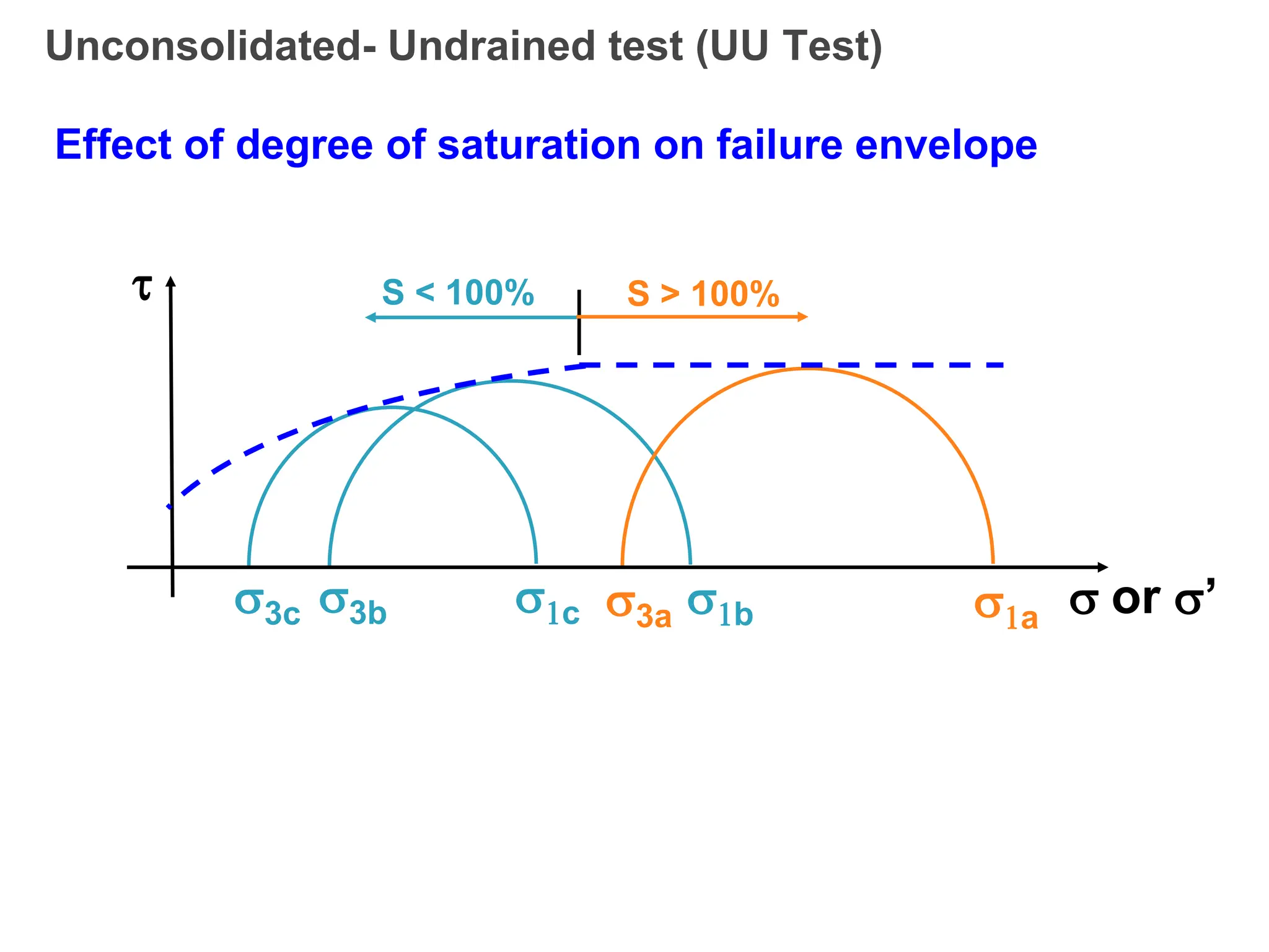
3b 1b
Unconsolidated- Undrainedtest (UU Test)
Effect of degree of saturation on failure envelope
3a 1a
3c 1c
or ’
S < 100% S > 100%
85.
Some practical applicationsof UU analysis for
clays
= in situ undrained
shear strength
Soft clay
1. Embankment constructed rapidly over a soft clay deposit
86.
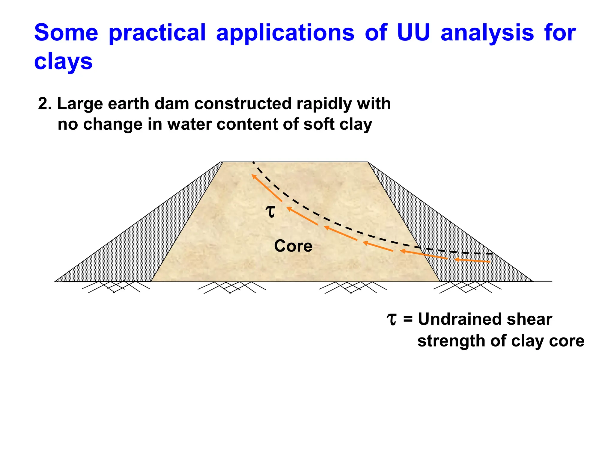
Some practical applicationsof UU analysis for
clays
2. Large earth dam constructed rapidly with
no change in water content of soft clay
Core
= Undrained shear
strength of clay core
87.
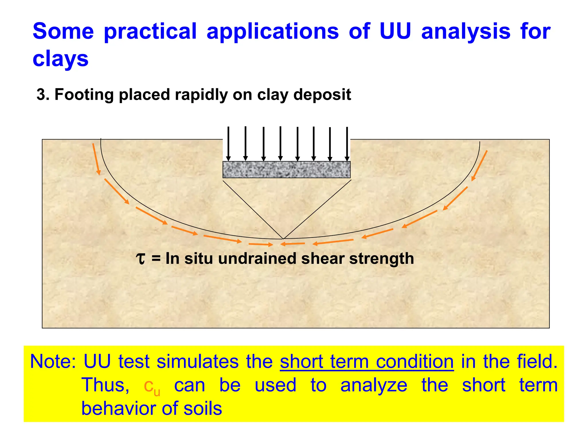
Some practical applicationsof UU analysis for
clays
3. Footing placed rapidly on clay deposit
= In situ undrained shear strength
Note: UU test simulates the short term condition in the field.
Thus, cu can be used to analyze the short term
behavior of soils
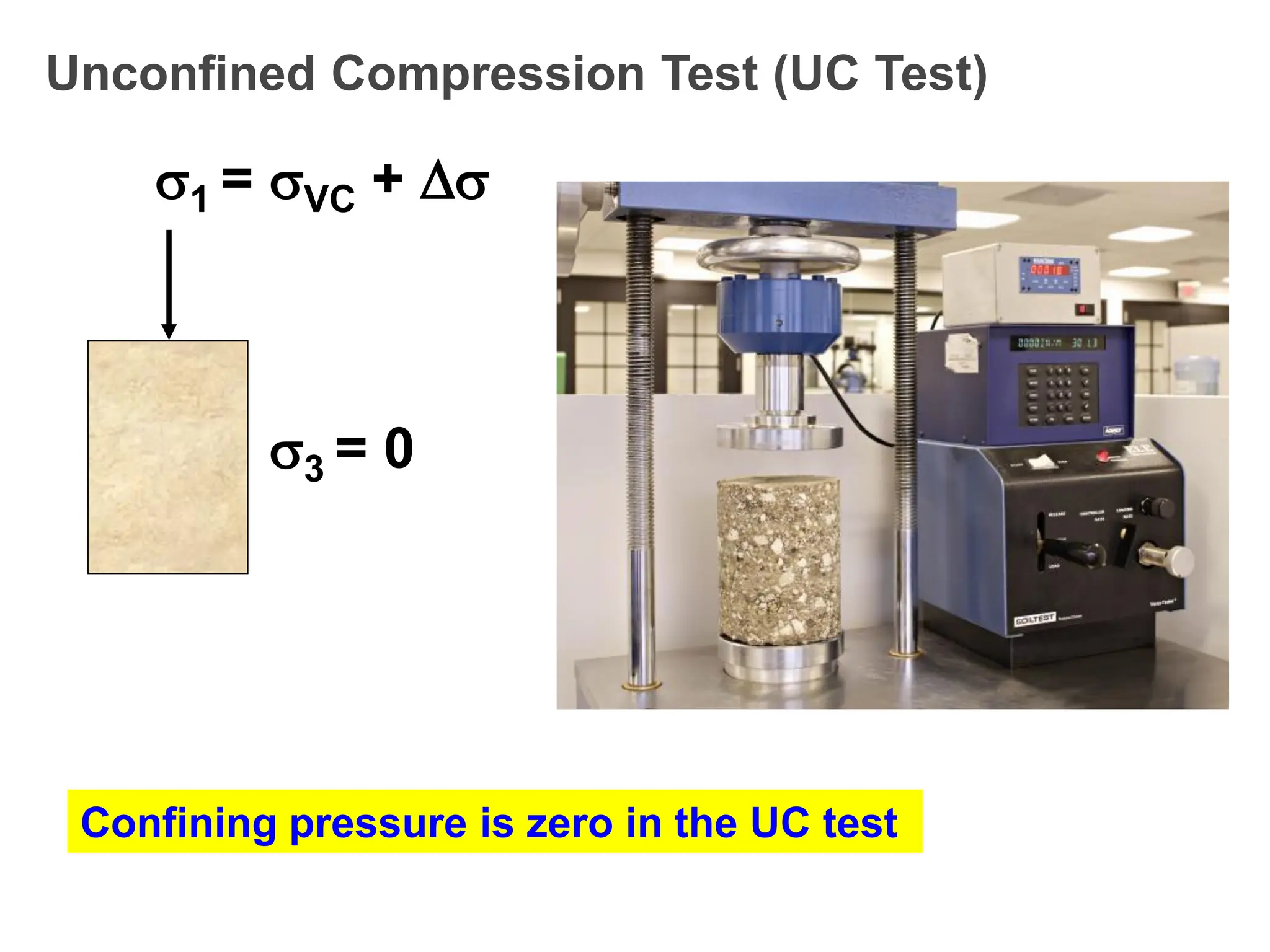
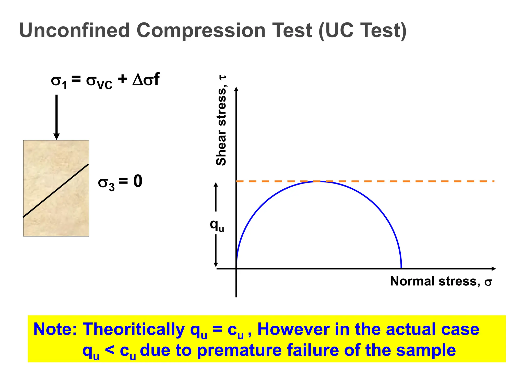
Unconfined Compression Test(UC Test)
1 = VC + f
3 = 0
Shear
stress,
Normal stress,
qu
Note: Theoritically qu = cu , However in the actual case
qu < cu due to premature failure of the sample
91.
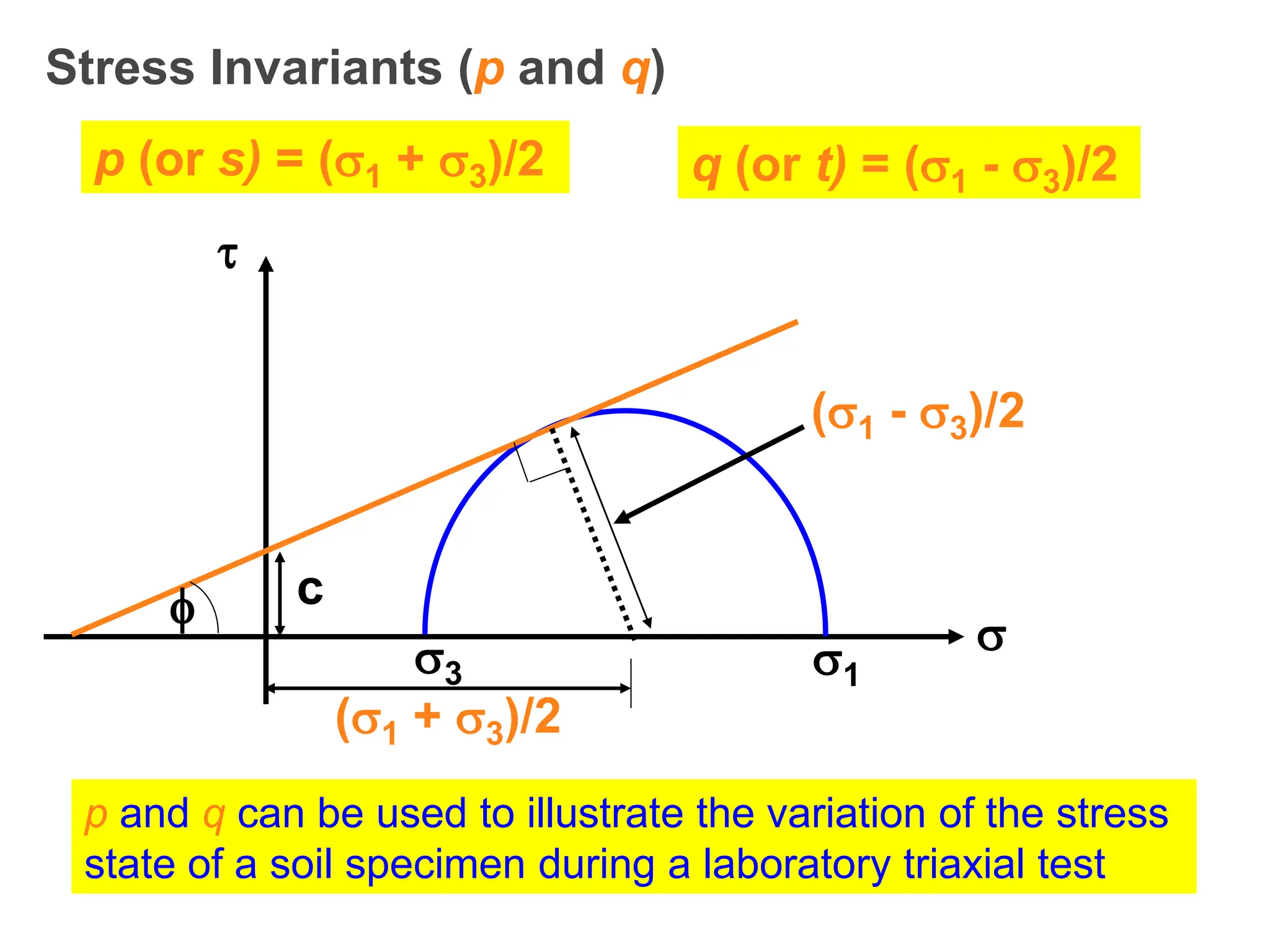
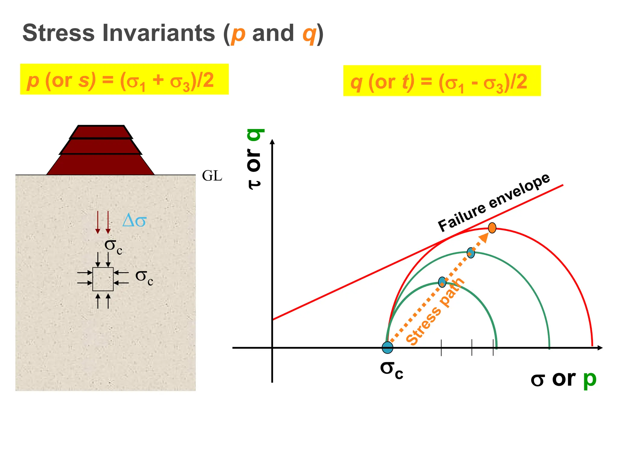
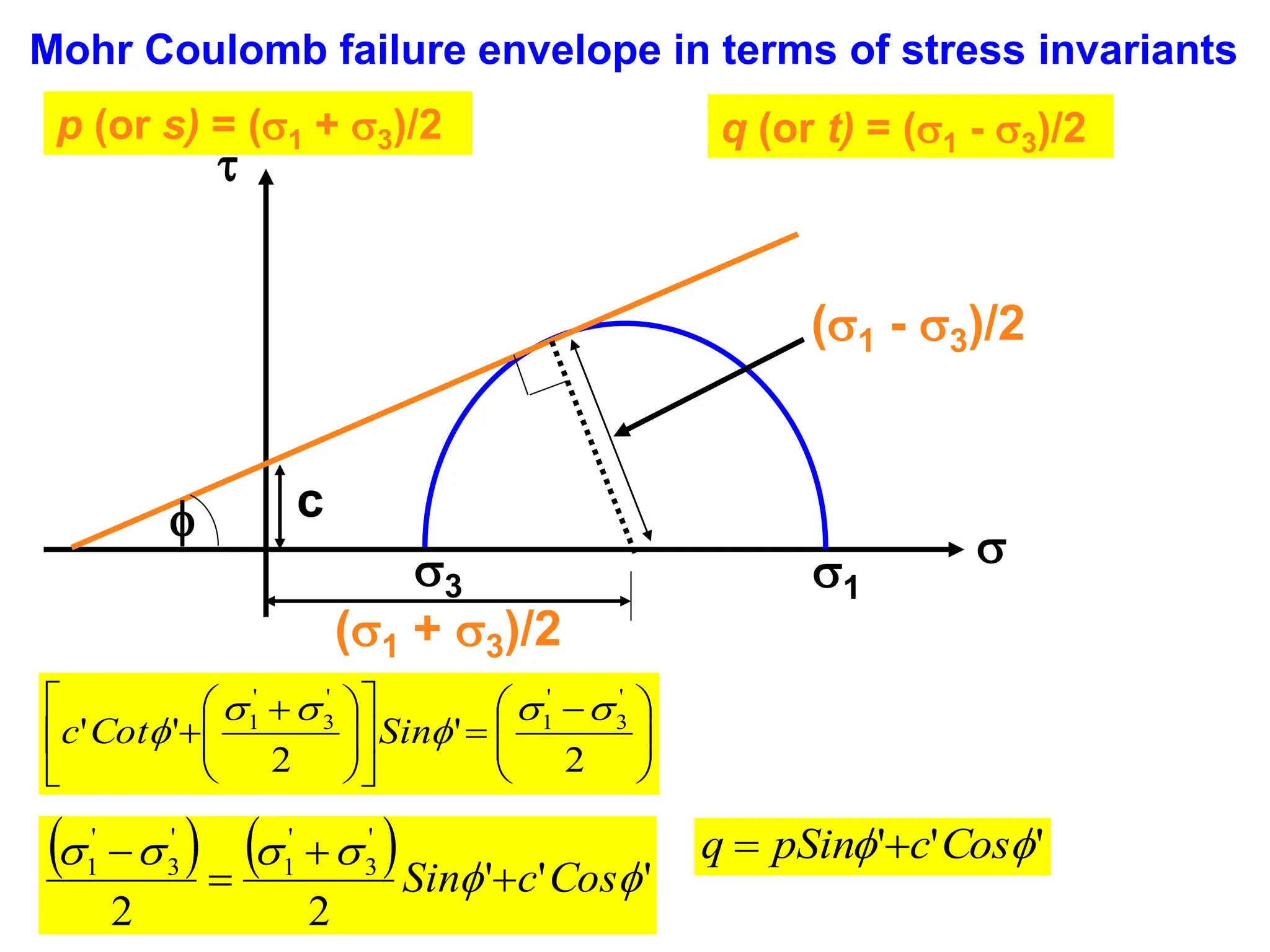
Stress Invariants (pand q)
p (or s) = (1 + 3)/2 q (or t) = (1 - 3)/2
3 1
(1 + 3)/2
(1 - 3)/2
c
p and q can be used to illustrate the variation of the stress
state of a soil specimen during a laboratory triaxial test
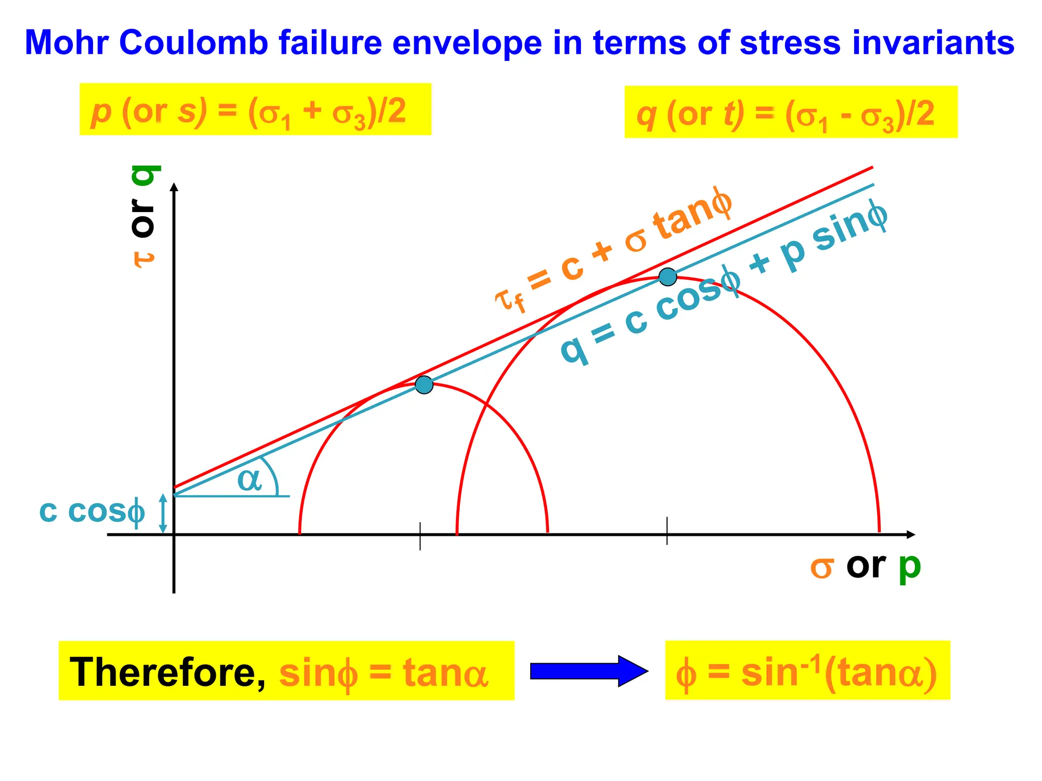
p (or s)= (1 + 3)/2 q (or t) = (1 - 3)/2
or
q
or p
Mohr Coulomb failure envelope in terms of stress invariants
a
Therefore, sin = tana = sin-1(tana)
c cos
95.
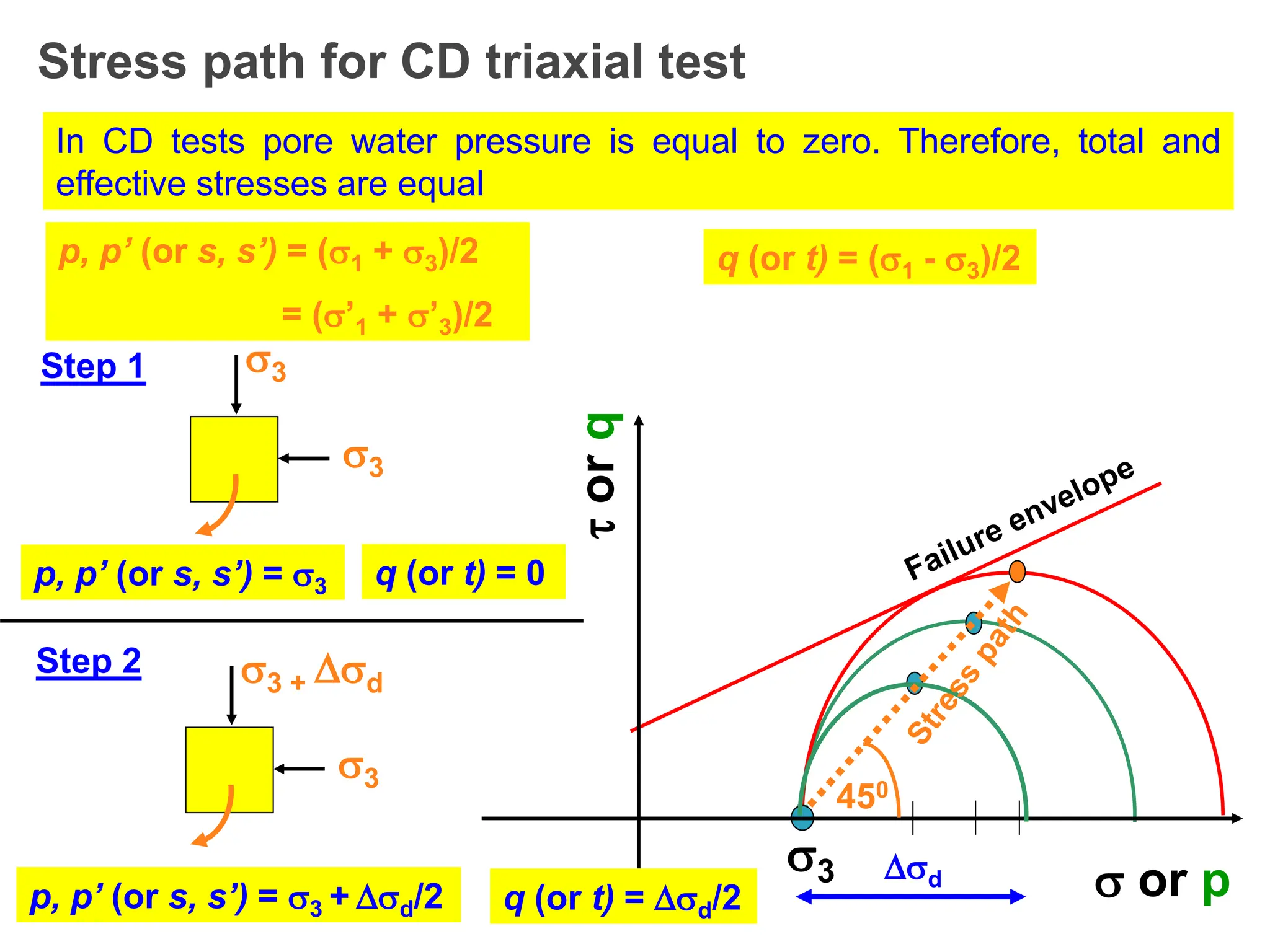
Stress path forCD triaxial test
3
p, p’ (or s, s’) = (1 + 3)/2
= (’1 + ’3)/2
q (or t) = (1 - 3)/2
or
q
or p
In CD tests pore water pressure is equal to zero. Therefore, total and
effective stresses are equal
Step 1 3
3
p, p’ (or s, s’) = 3 q (or t) = 0
Step 2 3 + d
3
p, p’ (or s, s’) = 3 + d/2 q (or t) = d/2
d
450
96.
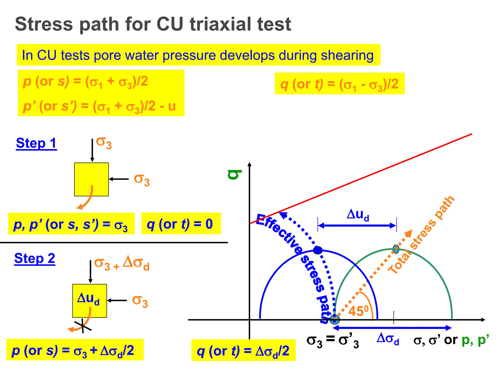
Stress path forCU triaxial test
3 = ’3
p (or s) = (1 + 3)/2
p’ (or s’) = (1 + 3)/2 - u
q (or t) = (1 - 3)/2
In CU tests pore water pressure develops during shearing
Step 1 3
3
p, p’ (or s, s’) = 3 q (or t) = 0
p (or s) = 3 + d/2
d
450
ud
Step 2 3 + d
3
ud
q
, ’ or p, p’
q (or t) = d/2
98.
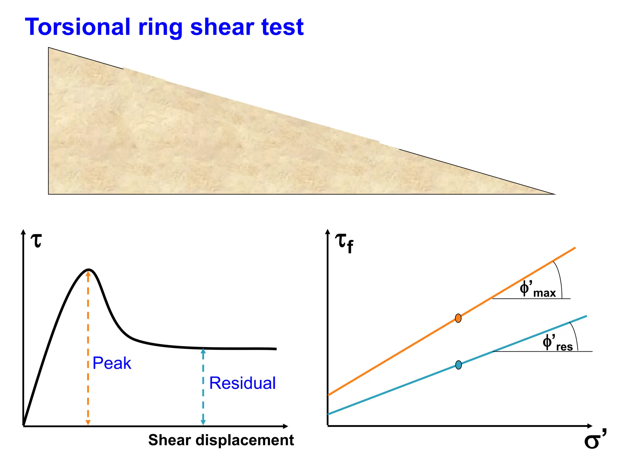
Other laboratory sheartests
Direct simple shear test
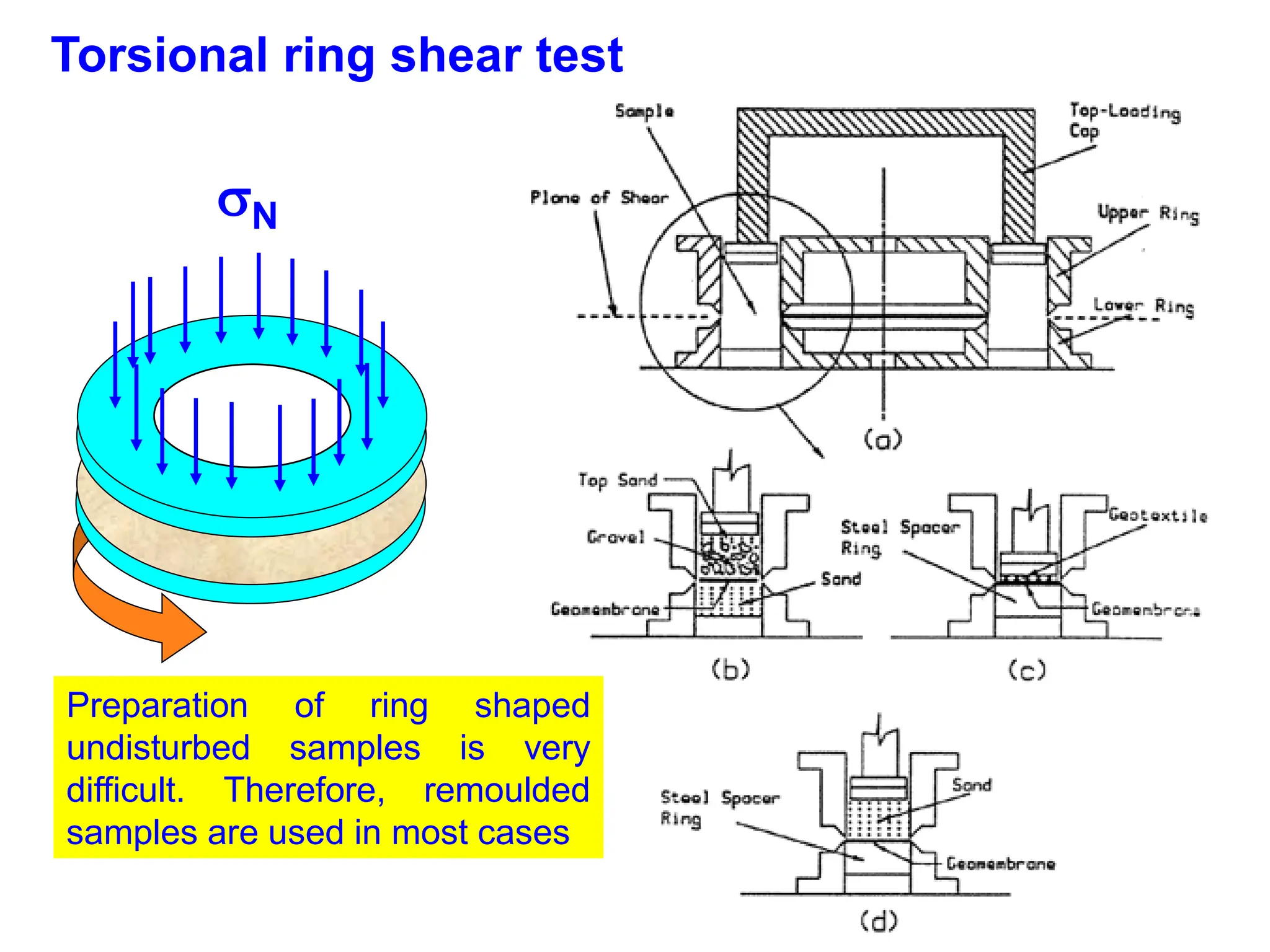
Torsional ring shear test
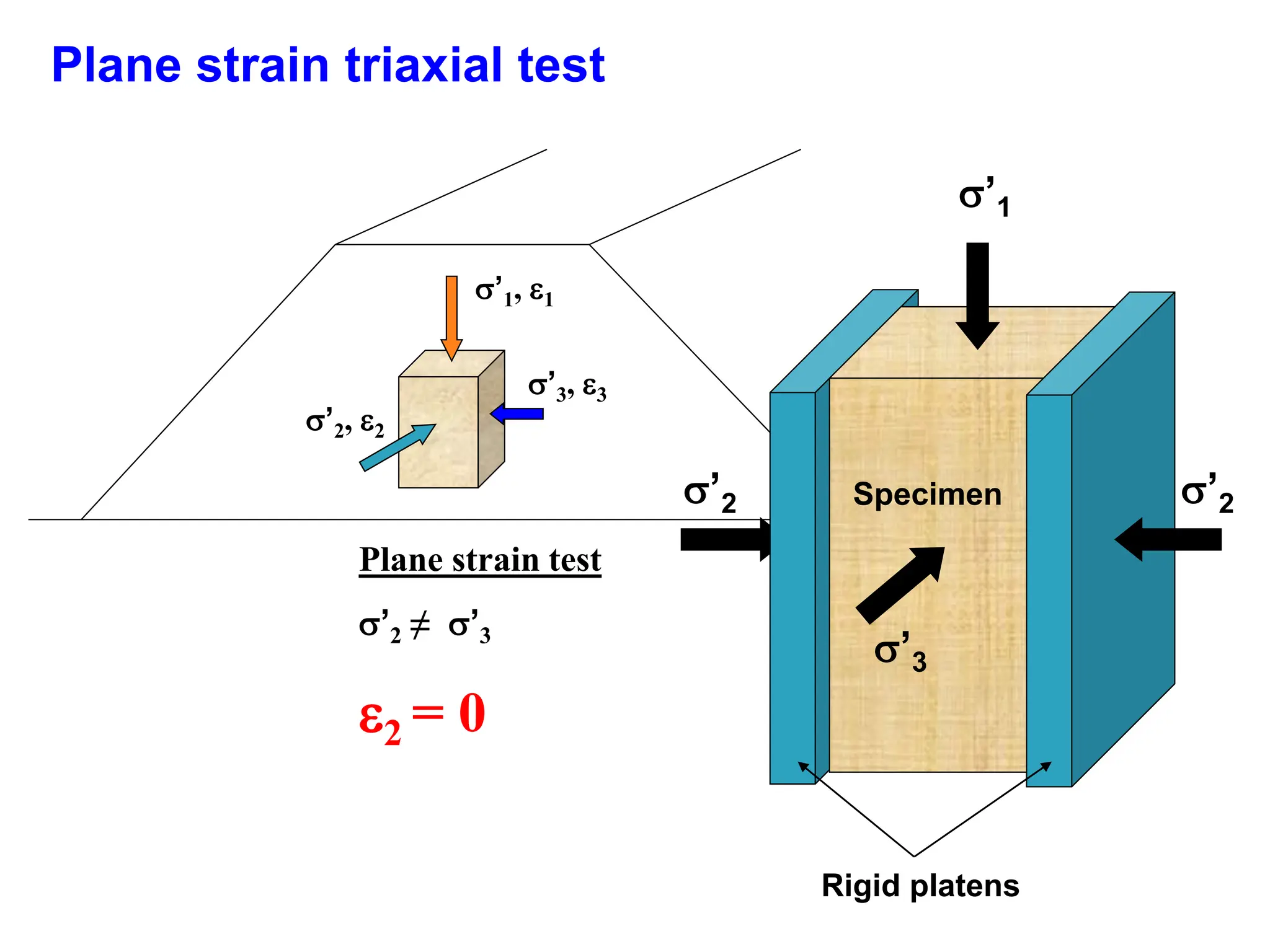
Plane strain triaxial test
99.
Other laboratory sheartests
Direct simple shear test
Torsional ring shear test
Plane strain triaxial test
100.
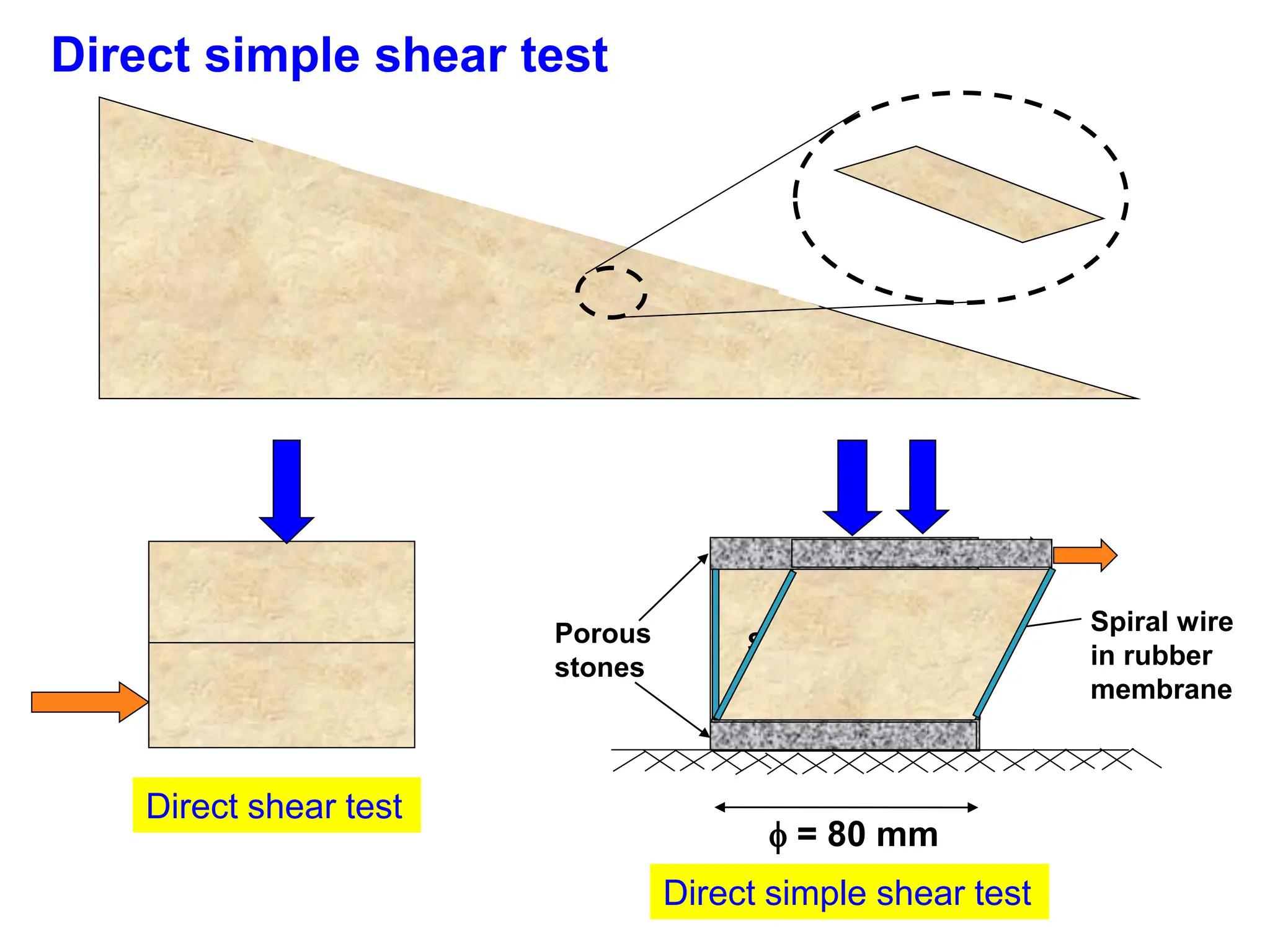
Direct simple sheartest
Direct shear test
= 80 mm
Soil specimen
Porous
stones
Spiral wire
in rubber
membrane
Direct simple shear test
101.
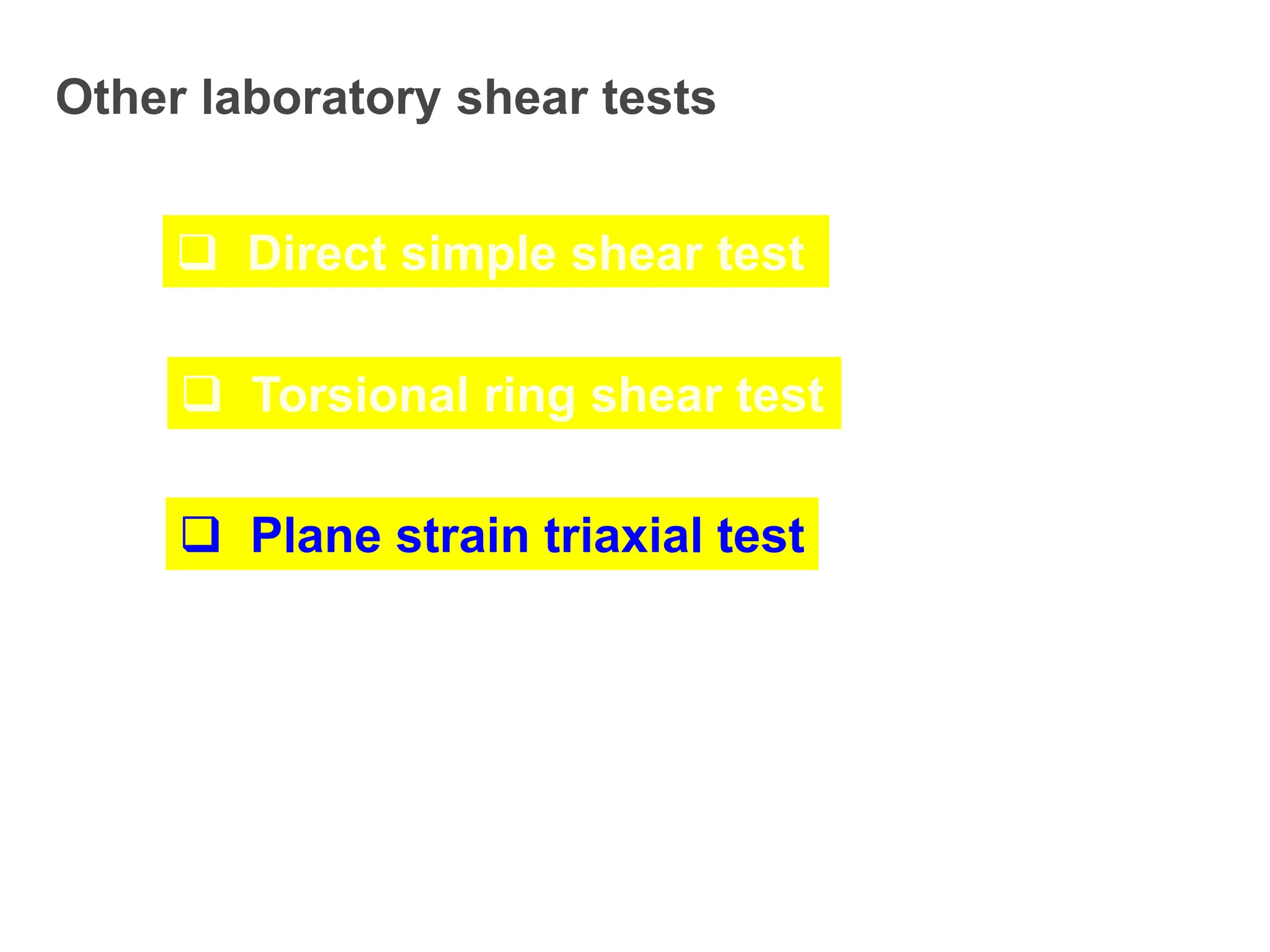
Other laboratory sheartests
Direct simple shear test
Torsional ring shear test
Plane strain triaxial test
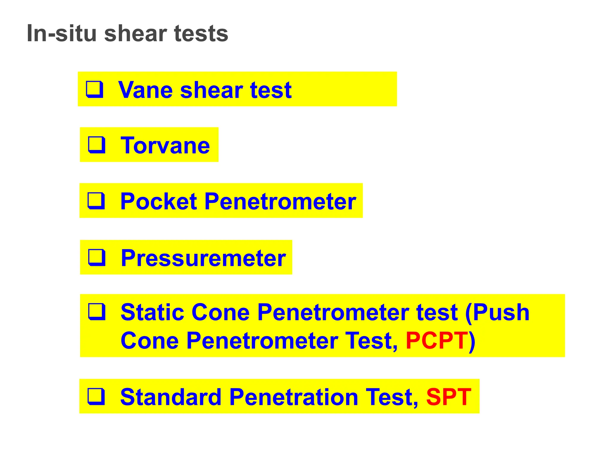
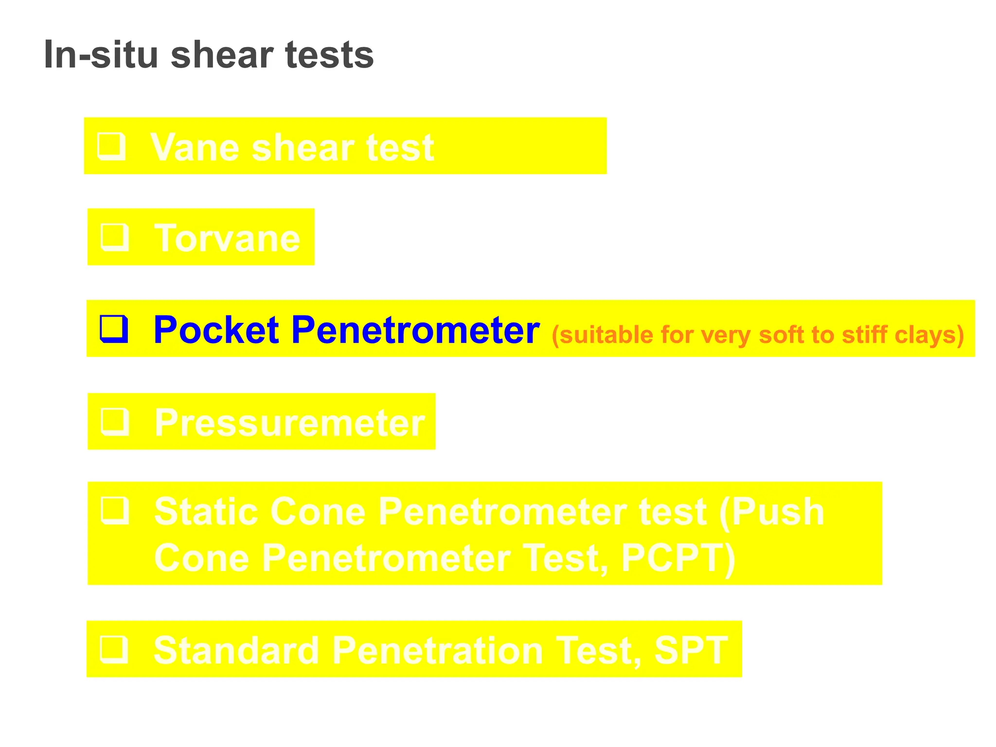
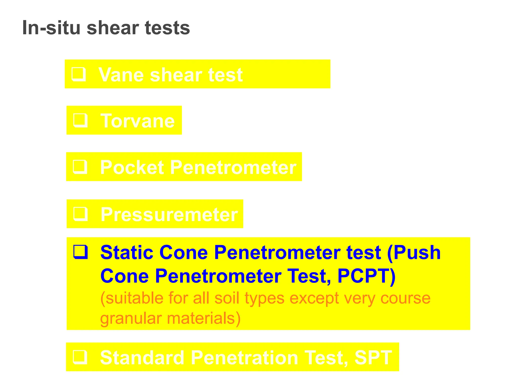
In-situ shear tests
Vane shear test
Torvane
Pocket Penetrometer
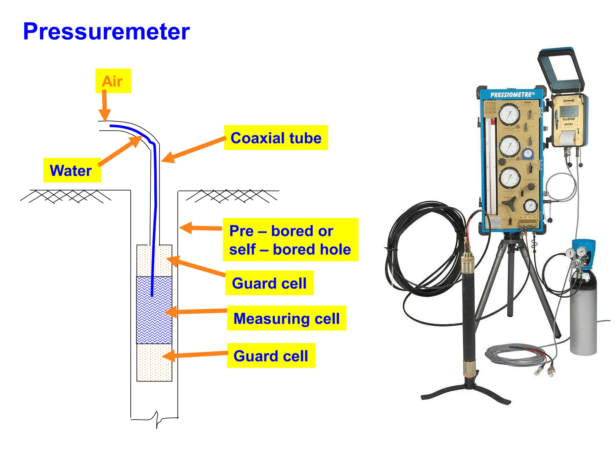
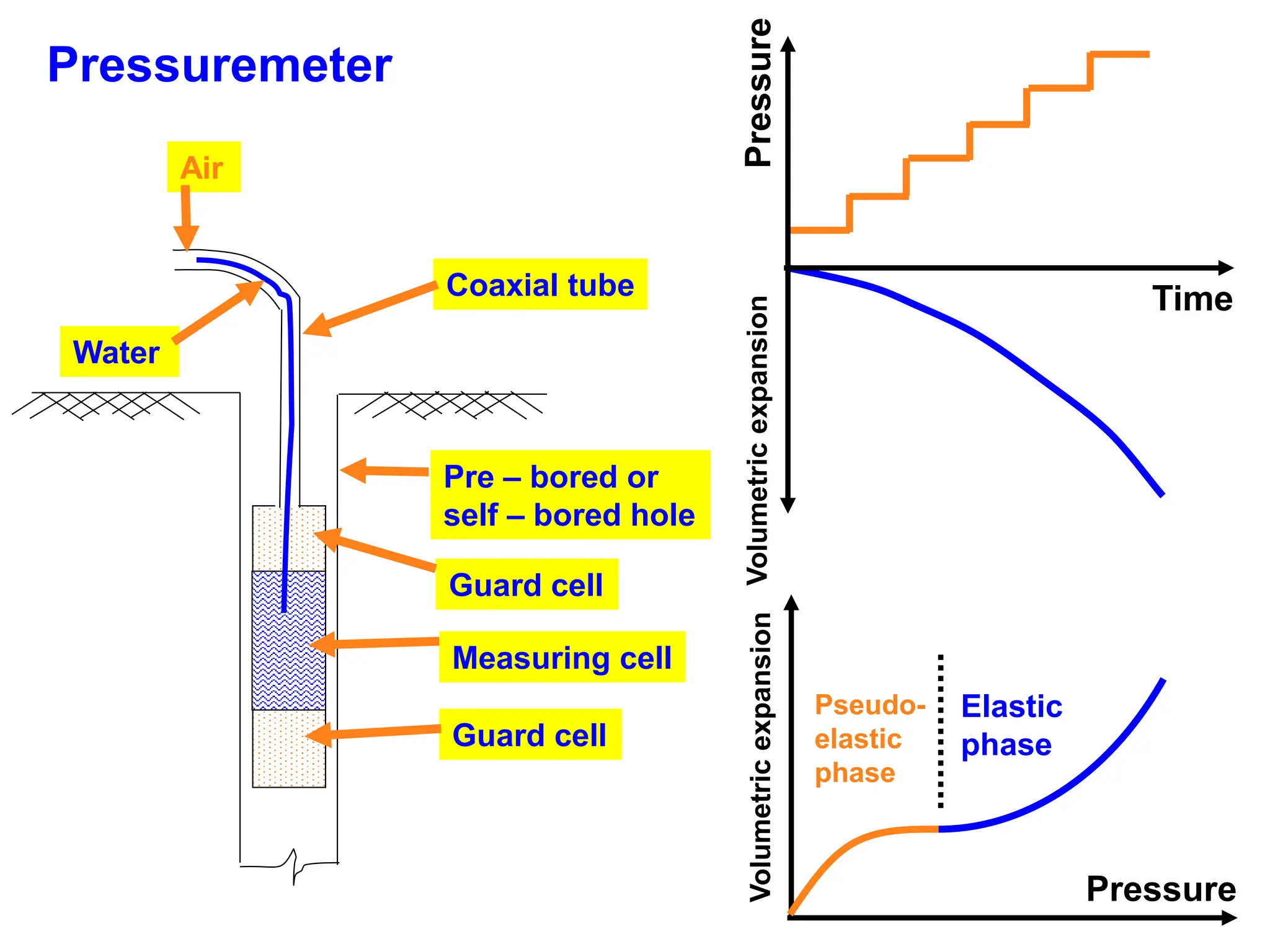
Pressuremeter
Static Cone Penetrometer test (Push
Cone Penetrometer Test, PCPT)
Standard Penetration Test, SPT
107.
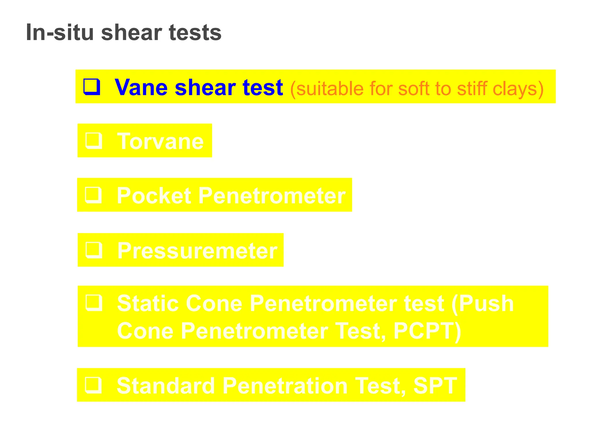
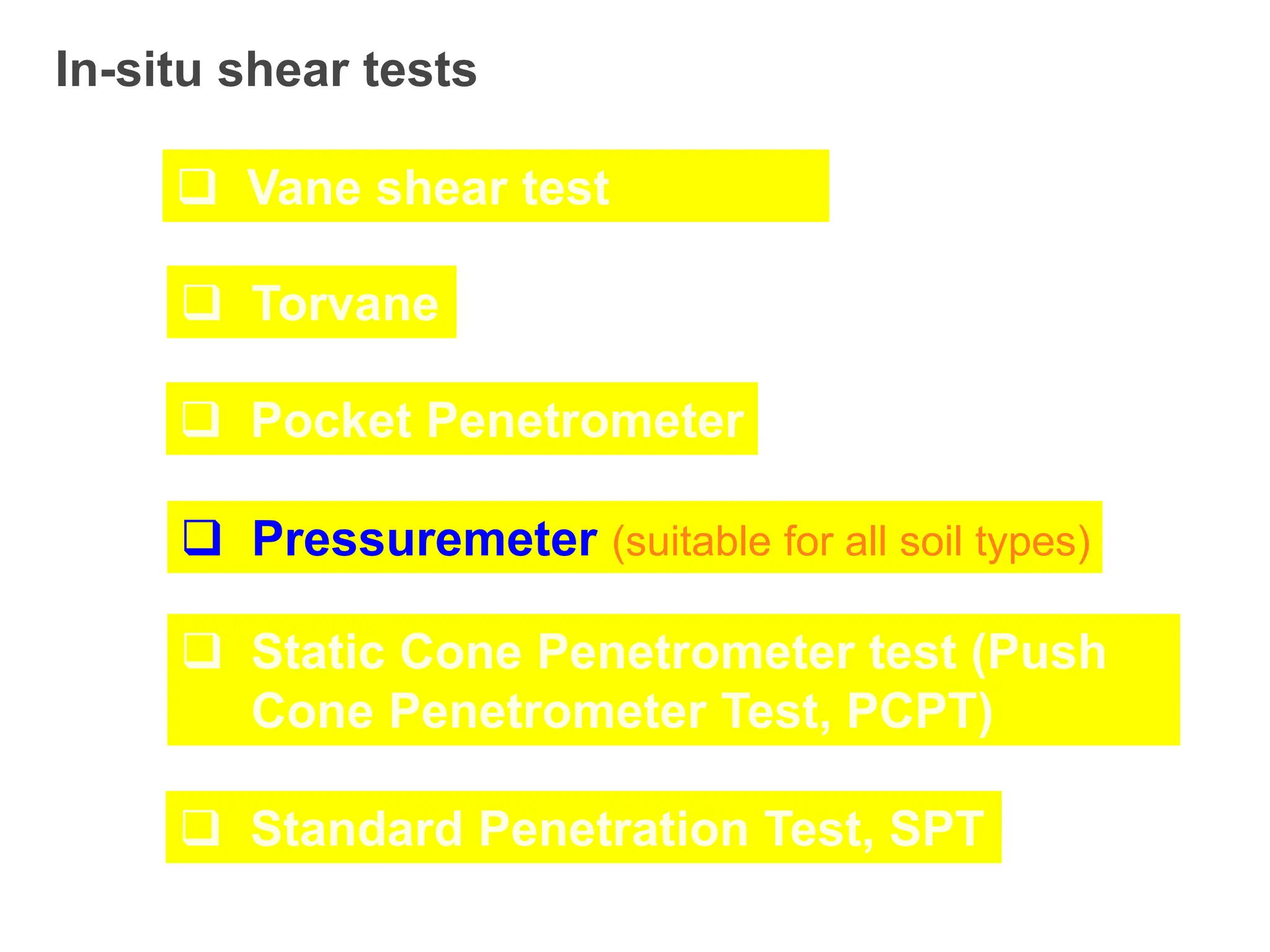
In-situ shear tests
Vane shear test (suitable for soft to stiff clays)
Torvane
Pocket Penetrometer
Pressuremeter
Static Cone Penetrometer test (Push
Cone Penetrometer Test, PCPT)
Standard Penetration Test, SPT
108.
PLAN VIEW
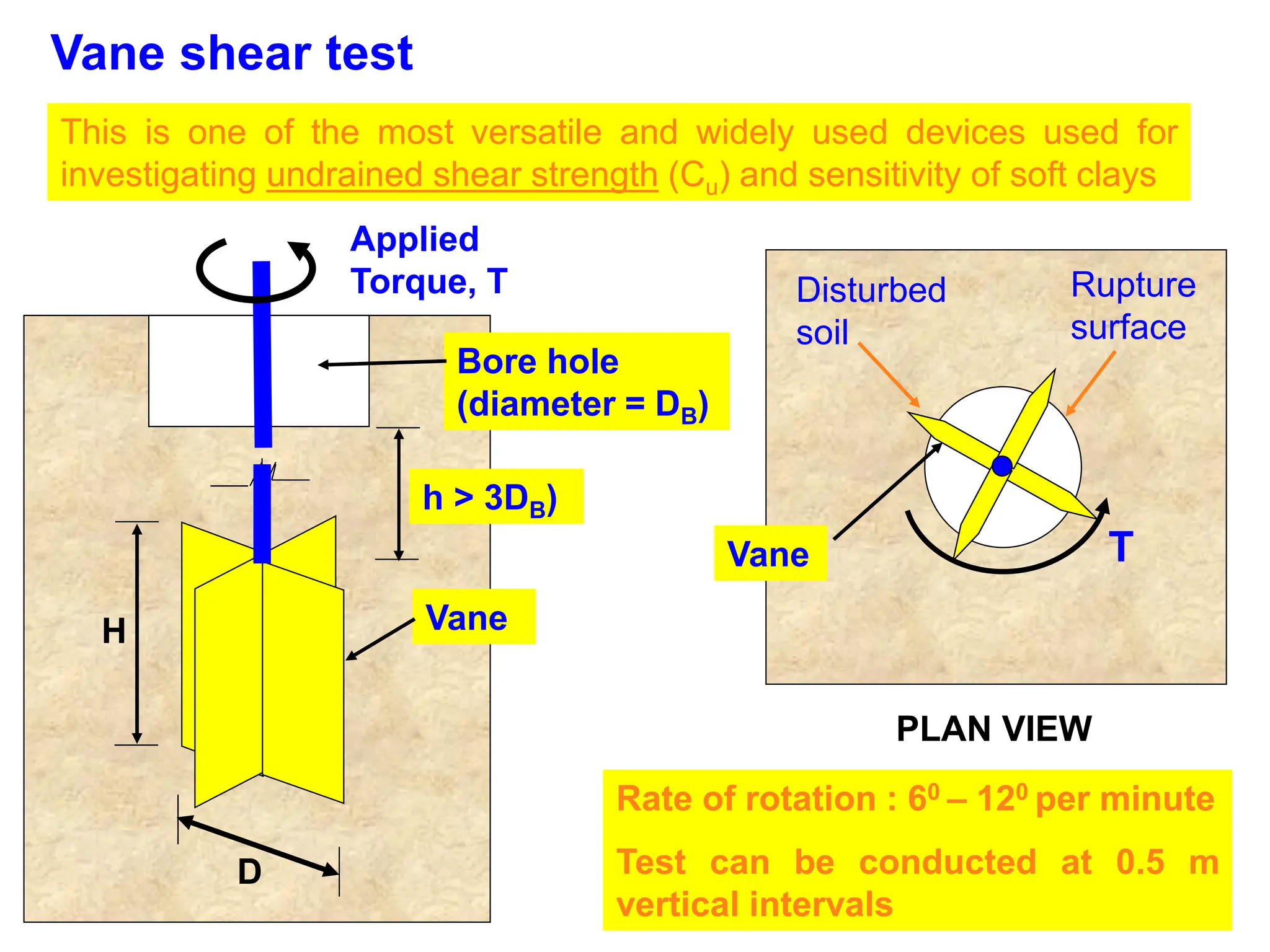
Vane sheartest
This is one of the most versatile and widely used devices used for
investigating undrained shear strength (Cu) and sensitivity of soft clays
Bore hole
(diameter = DB)
h > 3DB)
Vane
D
H
Applied
Torque, T
Vane T
Rupture
surface
Disturbed
soil
Rate of rotation : 60 – 120 per minute
Test can be conducted at 0.5 m
vertical intervals
109.
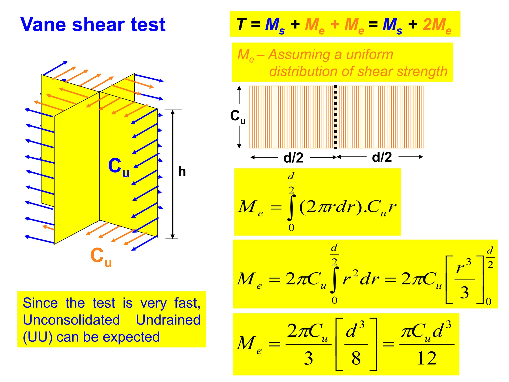
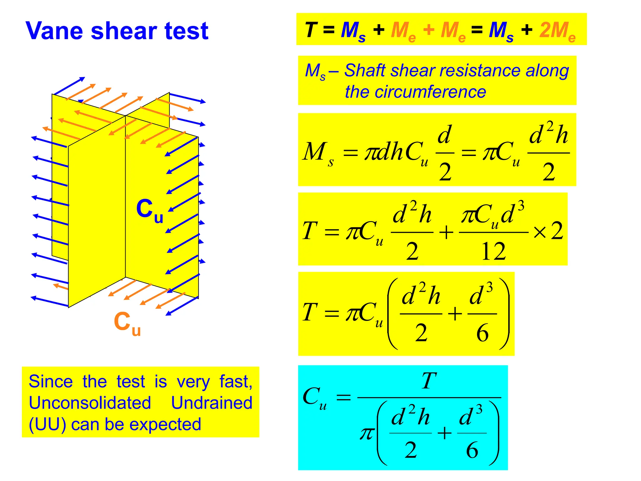
Vane shear test
Sincethe test is very fast,
Unconsolidated Undrained
(UU) can be expected
Cu
Cu
T = Ms + Me + Me = Ms + 2Me
Me – Assuming a uniform
distribution of shear strength
2
0
).
2
(
d
u
e r
C
rdr
M
2
0
3
2
0
2
3
2
2
d
u
d
u
e
r
C
dr
r
C
M
12
8
3
2 3
3
d
C
d
C
M u
u
e
d/2
d/2
Cu
h
110.
Vane shear test
Sincethe test is very fast,
Unconsolidated Undrained
(UU) can be expected
Cu
Cu
Ms – Shaft shear resistance along
the circumference
2
2
2
h
d
C
d
dhC
M u
u
s
2
12
2
3
2
d
C
h
d
C
T u
u
6
2
3
2
d
h
d
C
T u
6
2
3
2
d
h
d
T
Cu
T = Ms + Me + Me = Ms + 2Me
111.
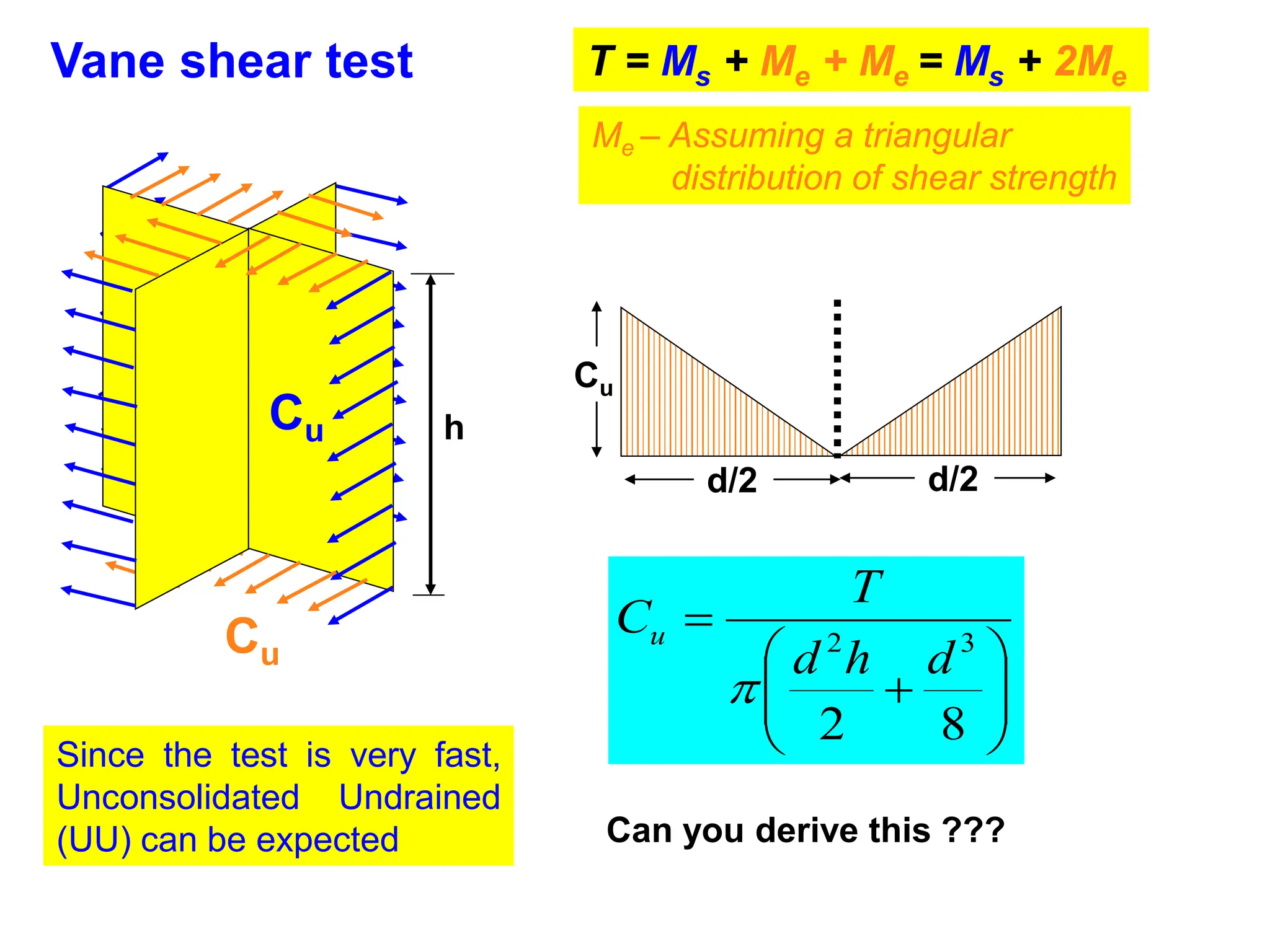
Vane shear test
Sincethe test is very fast,
Unconsolidated Undrained
(UU) can be expected
Cu
Cu
T = Ms + Me + Me = Ms + 2Me
Me – Assuming a triangular
distribution of shear strength
h
d/2
d/2
Cu
8
2
3
2
d
h
d
T
Cu
Can you derive this ???
112.
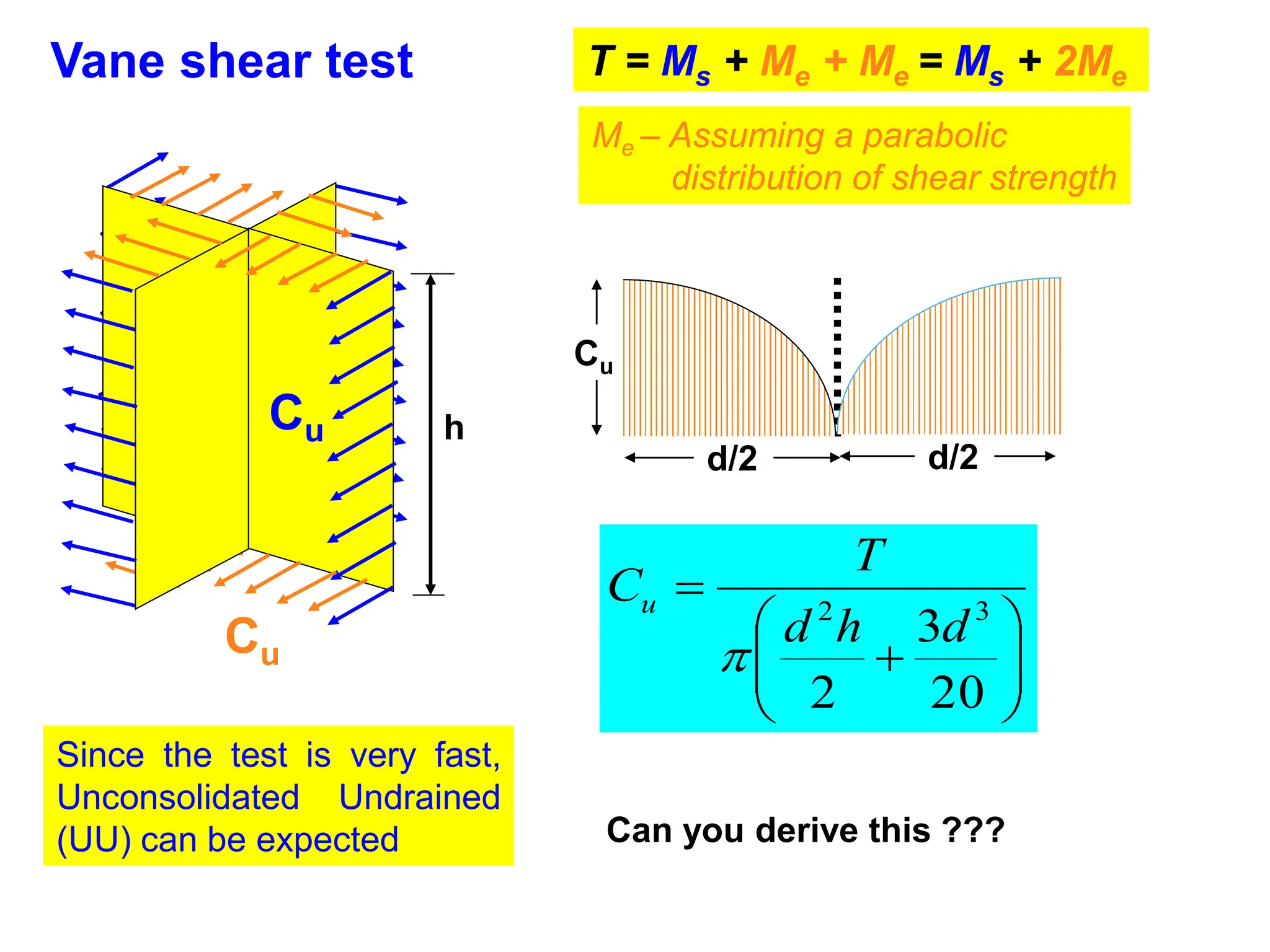
Vane shear test
Sincethe test is very fast,
Unconsolidated Undrained
(UU) can be expected
Cu
Cu
T = Ms + Me + Me = Ms + 2Me
Me – Assuming a parabolic
distribution of shear strength
h
20
3
2
3
2
d
h
d
T
Cu
Can you derive this ???
d/2
d/2
Cu
113.
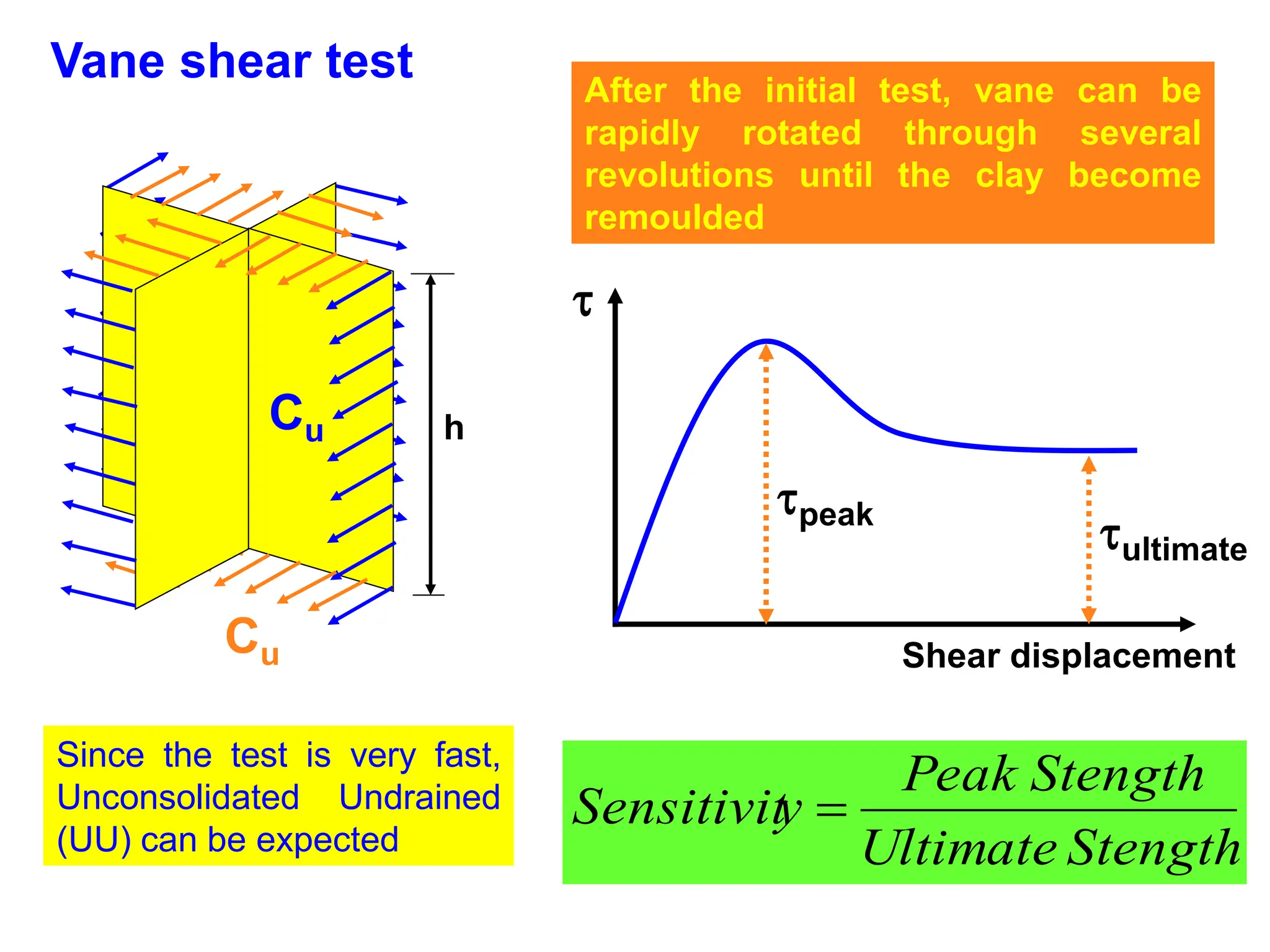
Vane shear test
Sincethe test is very fast,
Unconsolidated Undrained
(UU) can be expected
Cu
Cu
h
After the initial test, vane can be
rapidly rotated through several
revolutions until the clay become
remoulded
peak
ultimate
Shear displacement
Stength
Ultimate
Stength
Peak
y
Sensitivit
114.
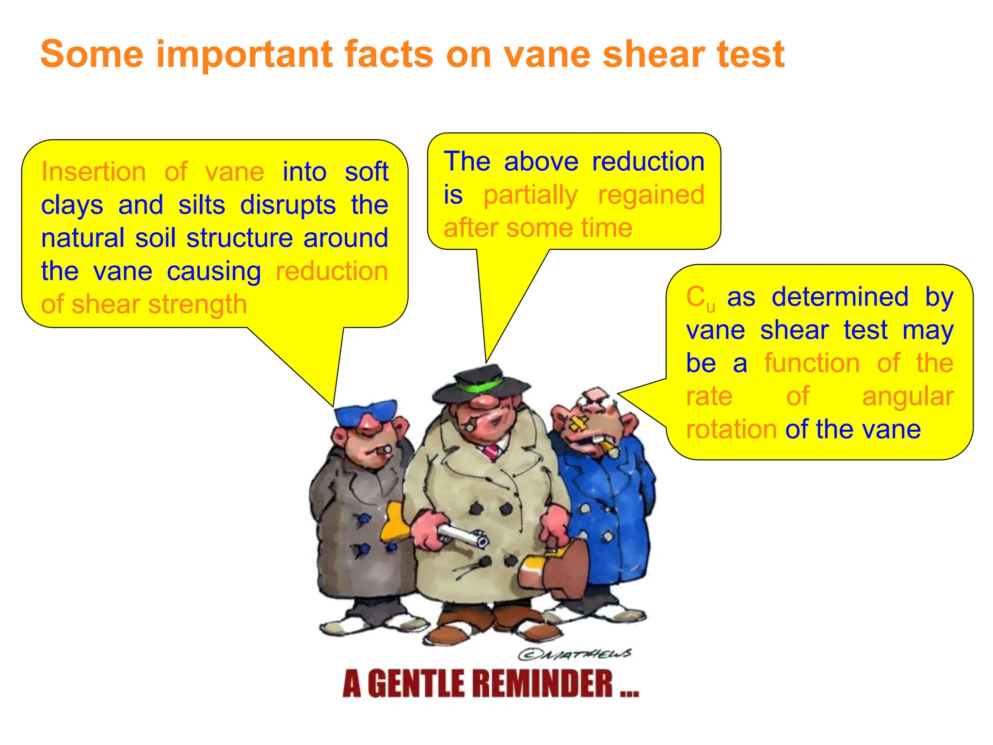
Some important factson vane shear test
Insertion of vane into soft
clays and silts disrupts the
natural soil structure around
the vane causing reduction
of shear strength
The above reduction
is partially regained
after some time
Cu as determined by
vane shear test may
be a function of the
rate of angular
rotation of the vane
115.
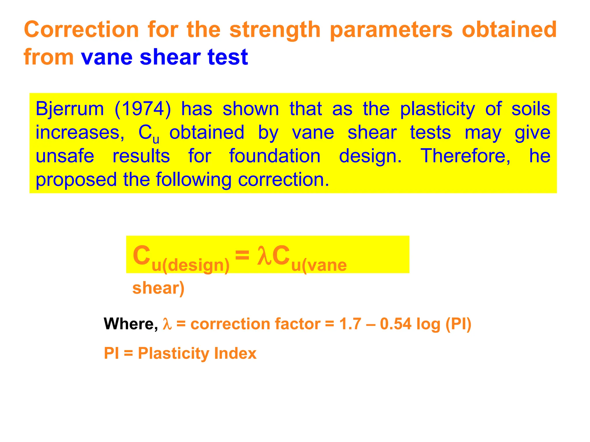
Correction for thestrength parameters obtained
from vane shear test
Bjerrum (1974) has shown that as the plasticity of soils
increases, Cu obtained by vane shear tests may give
unsafe results for foundation design. Therefore, he
proposed the following correction.
Cu(design) = lCu(vane
shear)
Where, l = correction factor = 1.7 – 0.54 log (PI)
PI = Plasticity Index
116.
In-situ shear tests
Vane shear test
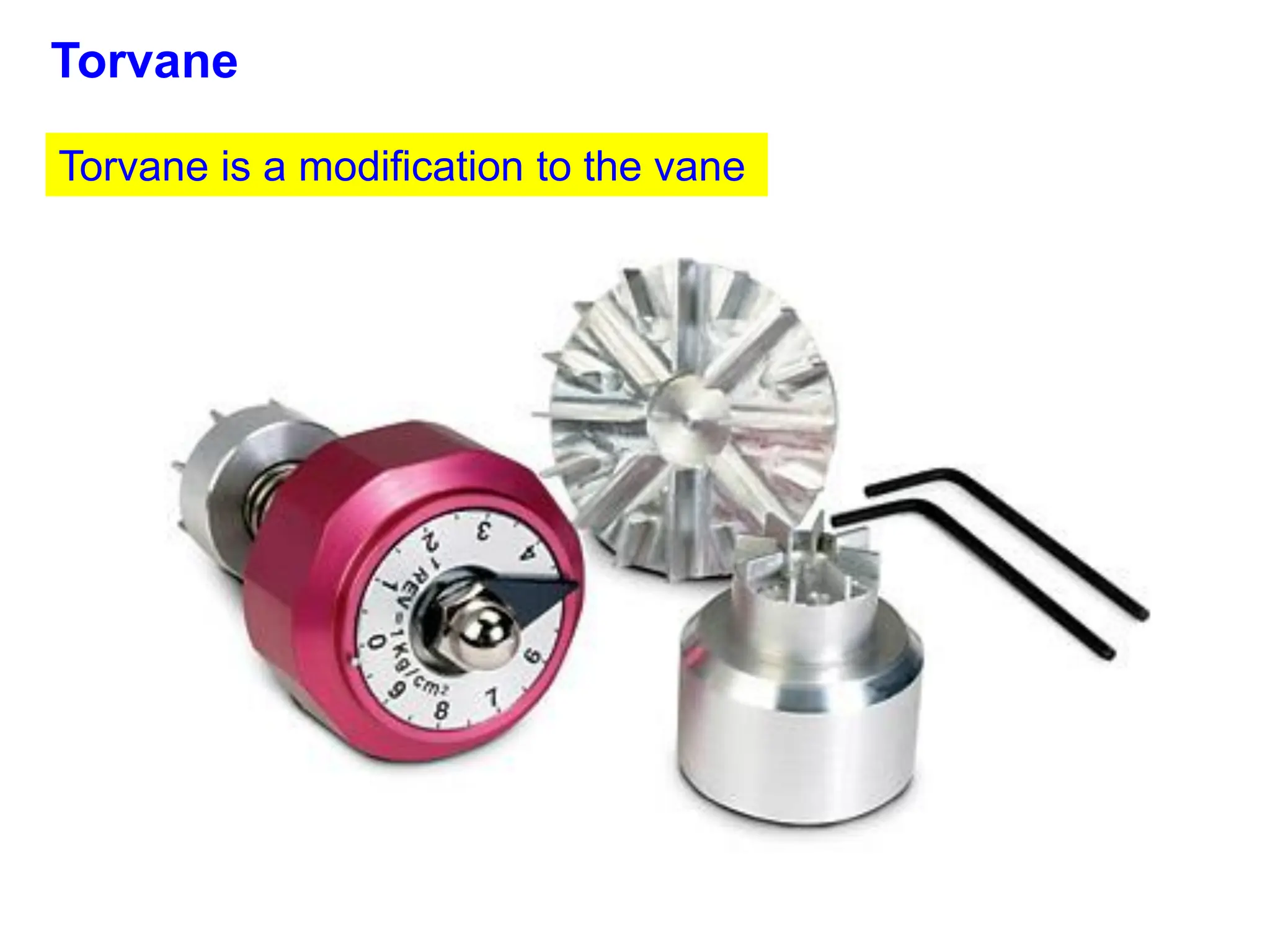
Torvane (suitable for very soft to stiff clays)
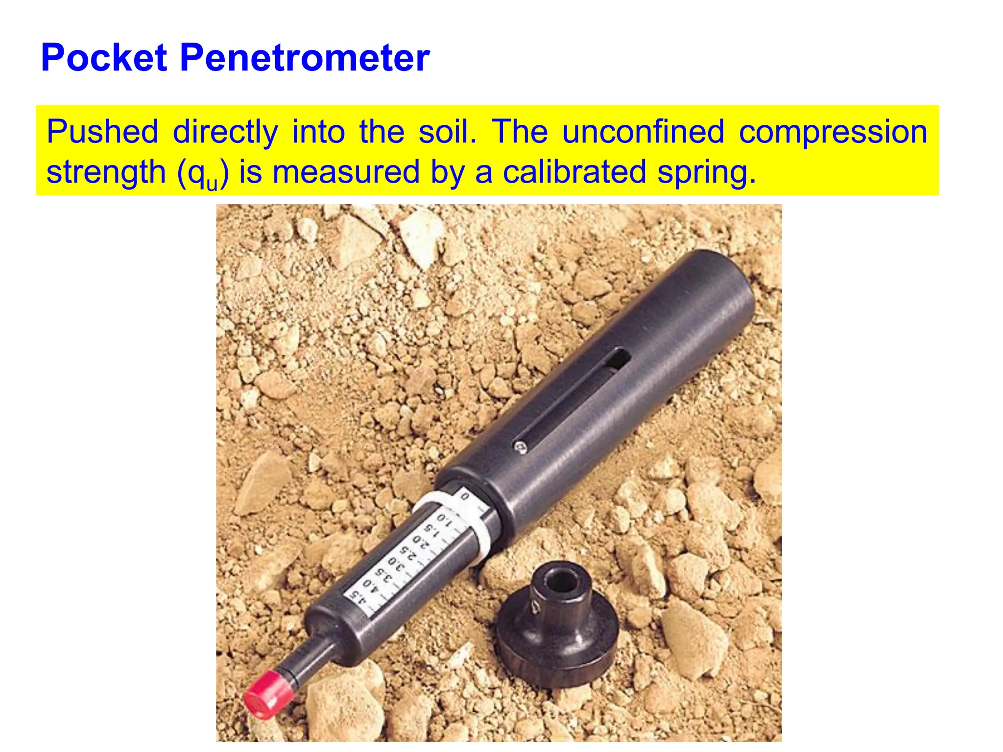
Pocket Penetrometer
Pressuremeter
Static Cone Penetrometer test (Push
Cone Penetrometer Test, PCPT)
Standard Penetration Test, SPT
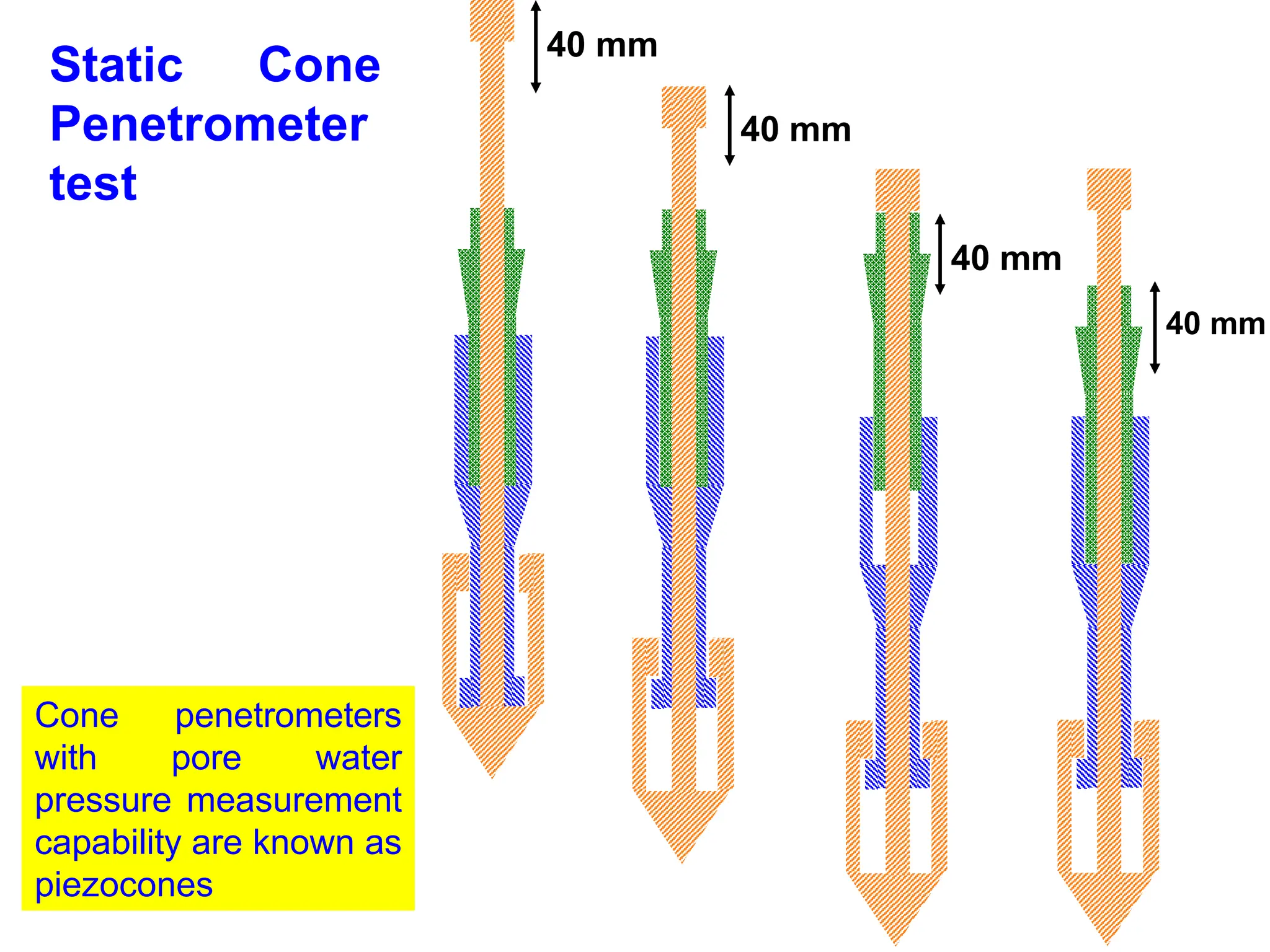
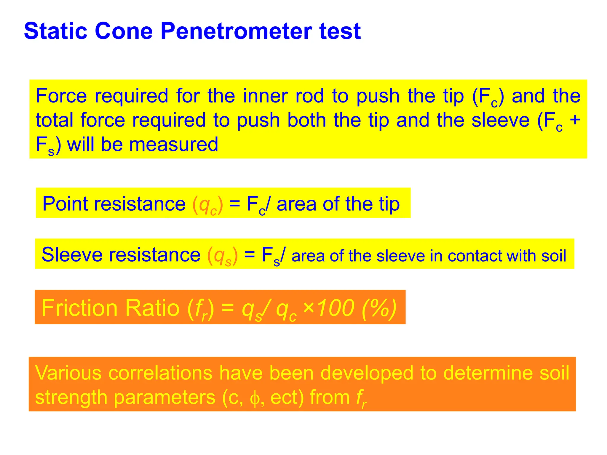
Static Cone Penetrometertest
Force required for the inner rod to push the tip (Fc) and the
total force required to push both the tip and the sleeve (Fc +
Fs) will be measured
Point resistance (qc) = Fc/ area of the tip
Sleeve resistance (qs) = Fs/ area of the sleeve in contact with soil
Friction Ratio (fr) = qs/ qc ×100 (%)
Various correlations have been developed to determine soil
strength parameters (c, , ect) from fr
127.
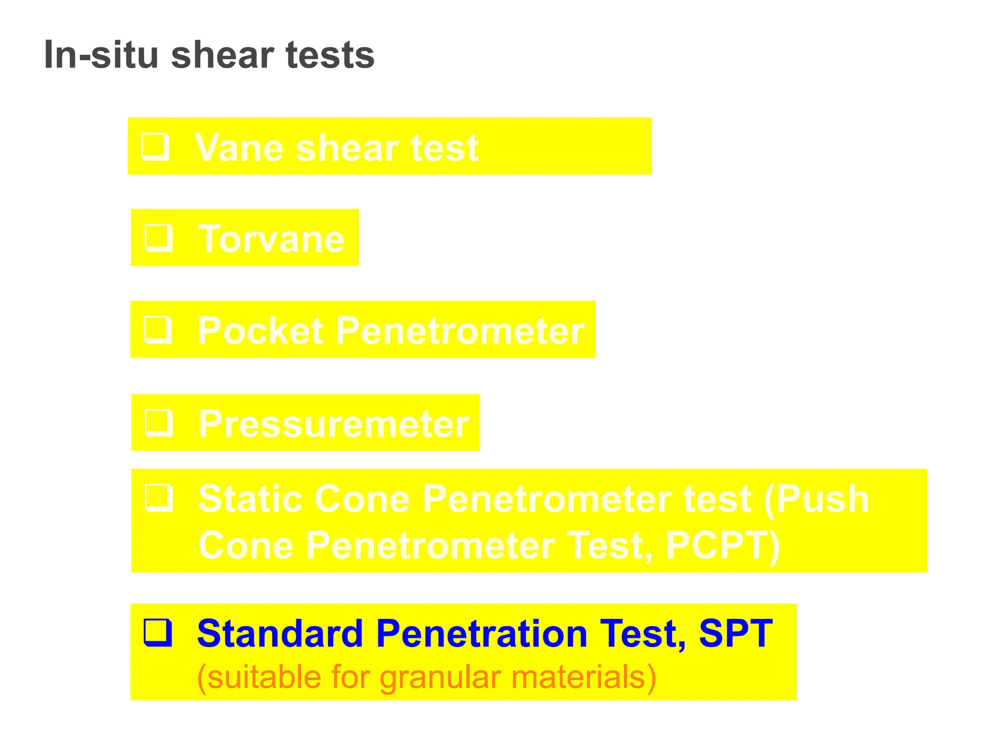
In-situ shear tests
Vane shear test
Torvane
Pocket Penetrometer
Pressuremeter
Static Cone Penetrometer test (Push
Cone Penetrometer Test, PCPT)
Standard Penetration Test, SPT
(suitable for granular materials)
128.
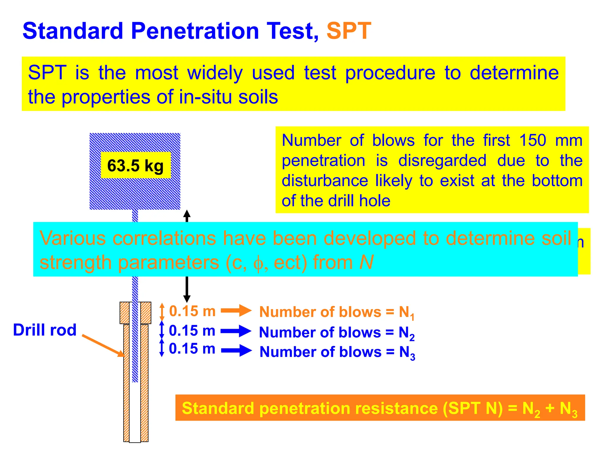
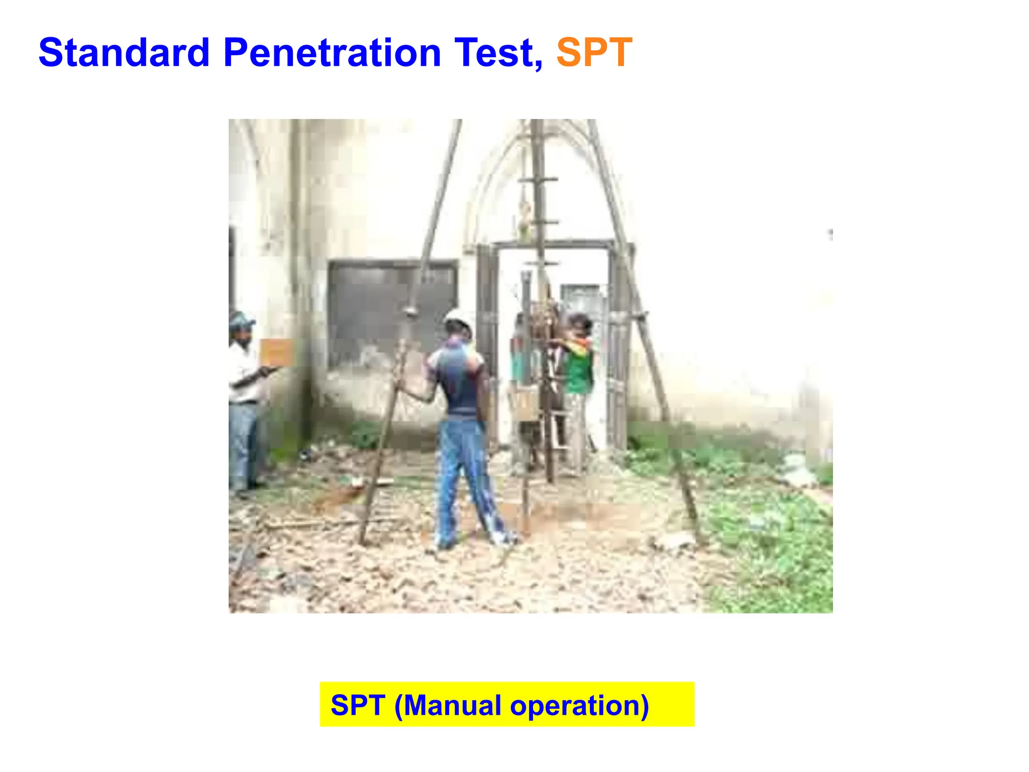
Standard Penetration Test,SPT
SPT is the most widely used test procedure to determine
the properties of in-situ soils
63.5 kg
0.76 m
Drill rod
0.15 m
0.15 m
0.15 m
Number of blows = N1
Number of blows = N2
Number of blows = N3
Standard penetration resistance (SPT N) = N2 + N3
Number of blows for the first 150 mm
penetration is disregarded due to the
disturbance likely to exist at the bottom
of the drill hole
The test can be conducted at every 1m
vertical intervals
Various correlations have been developed to determine soil
strength parameters (c, , ect) from N
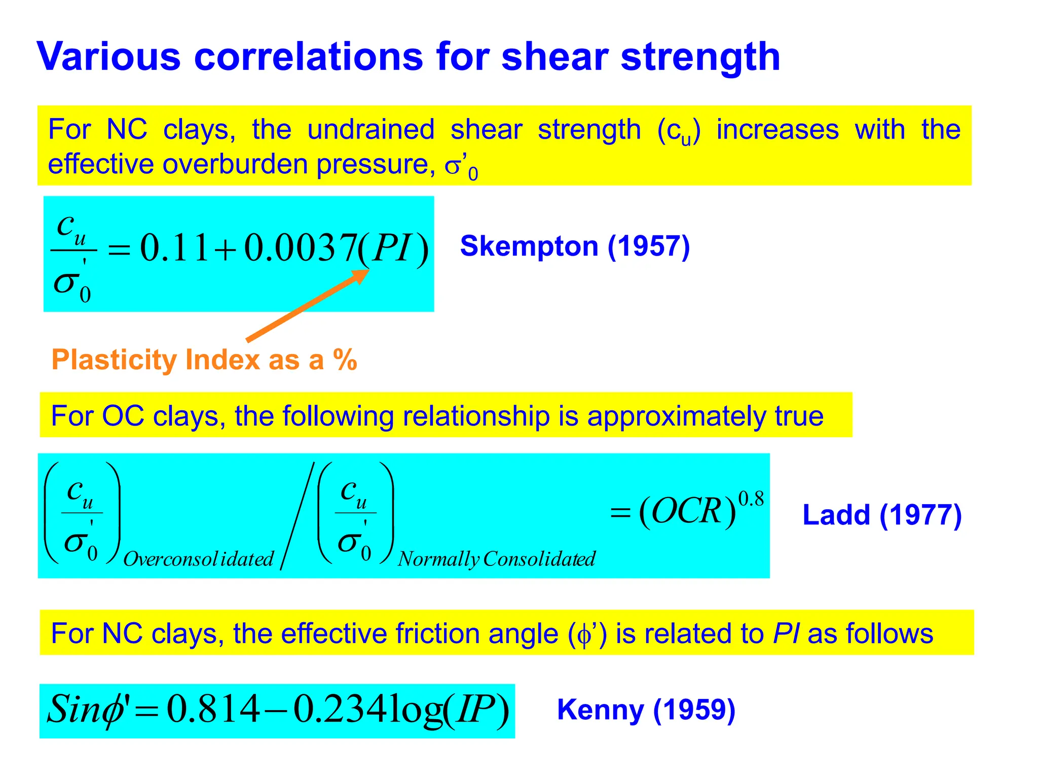
Various correlations forshear strength
For NC clays, the undrained shear strength (cu) increases with the
effective overburden pressure, ’0
)
(
0037
.
0
11
.
0
'
0
PI
cu
Skempton (1957)
Plasticity Index as a %
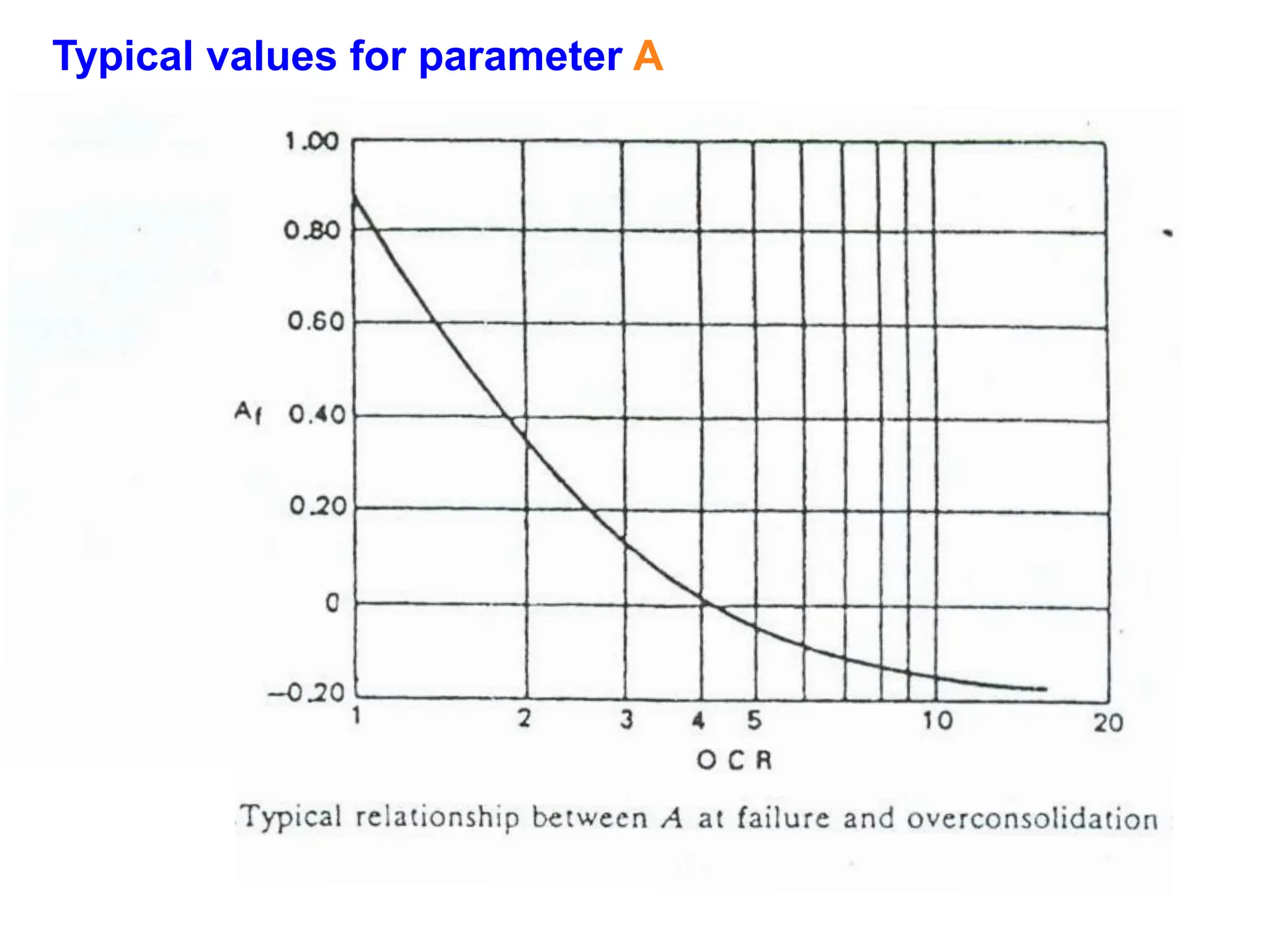
For OC clays, the following relationship is approximately true
8
.
0
'
0
'
0
)
(OCR
c
c
ed
Consolidat
Normally
u
idated
Overconsol
u
Ladd (1977)
For NC clays, the effective friction angle (’) is related to PI as follows
)
log(
234
.
0
814
.
0
' IP
Sin
Kenny (1959)
131.
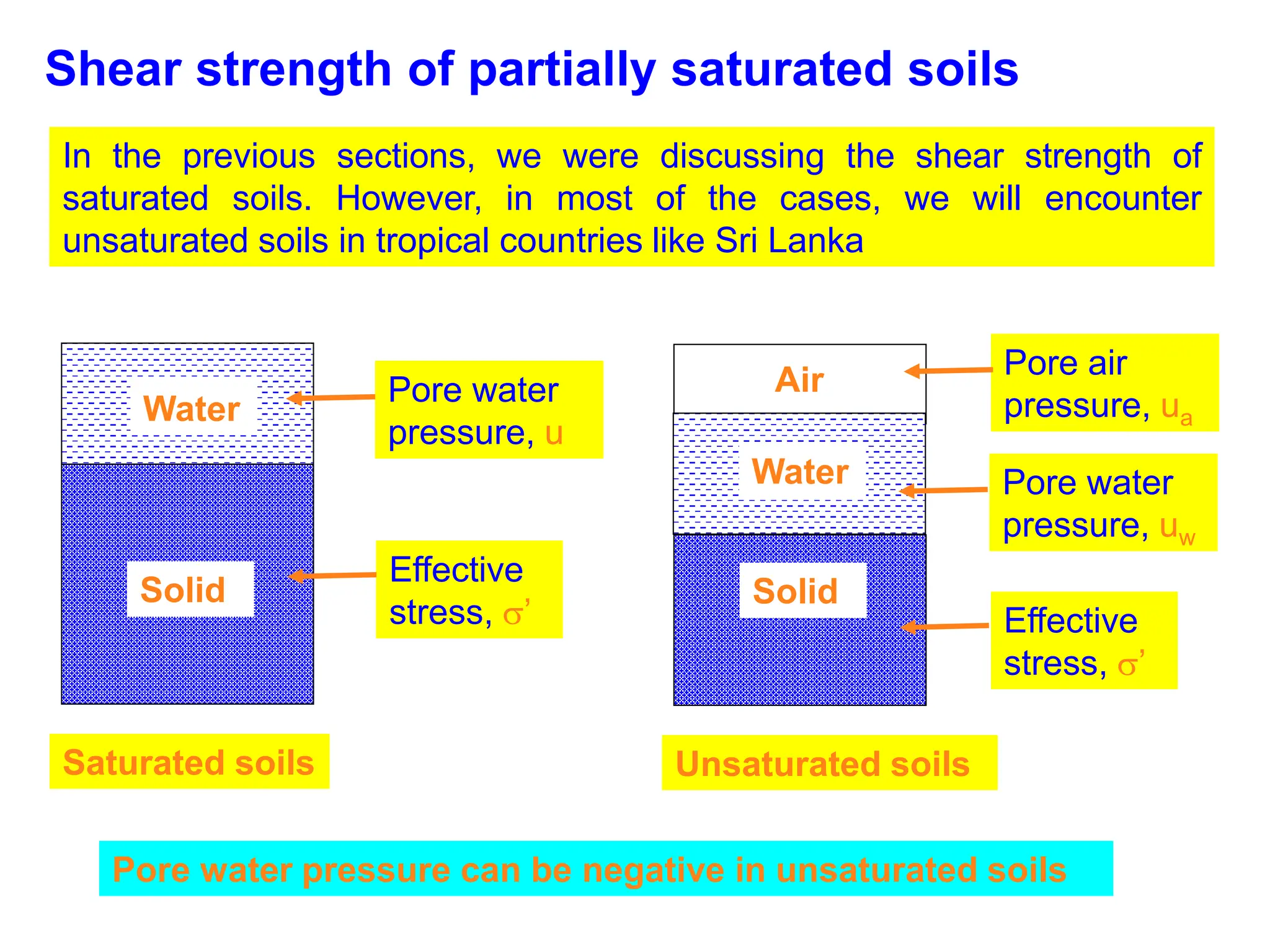
Shear strength ofpartially saturated soils
In the previous sections, we were discussing the shear strength of
saturated soils. However, in most of the cases, we will encounter
unsaturated soils in tropical countries like Sri Lanka
Solid
Water
Saturated soils
Pore water
pressure, u
Effective
stress, ’
Solid
Unsaturated soils
Pore water
pressure, uw
Effective
stress, ’
Water
Air Pore air
pressure, ua
Pore water pressure can be negative in unsaturated soils
132.
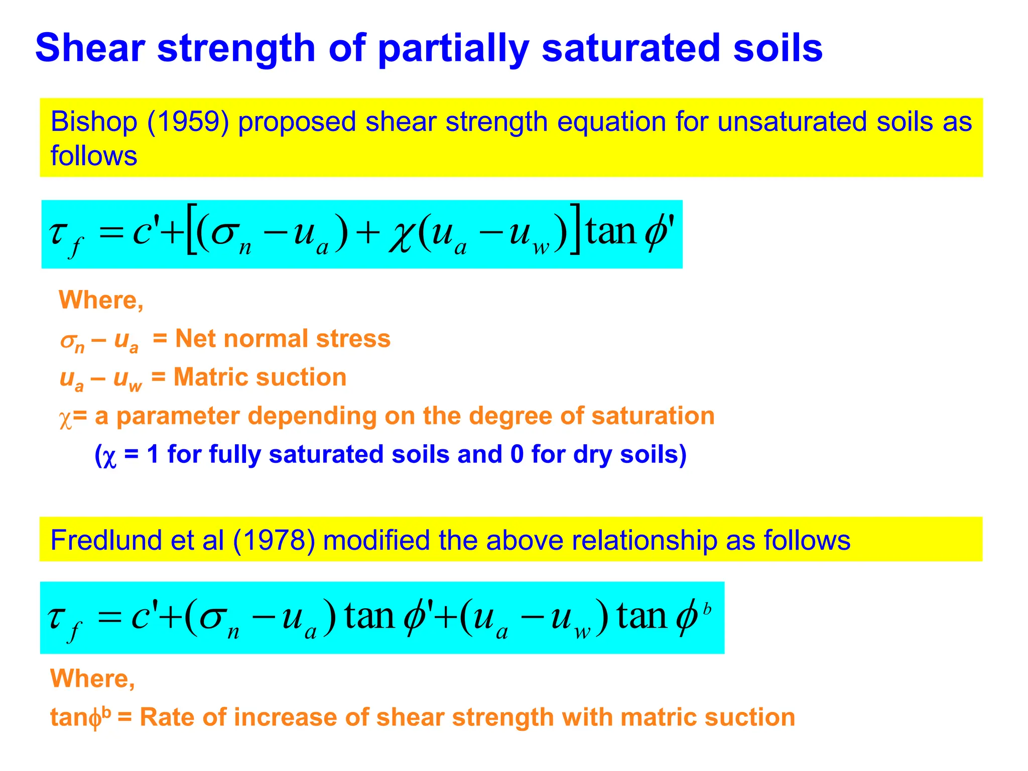
Shear strength ofpartially saturated soils
Bishop (1959) proposed shear strength equation for unsaturated soils as
follows
'
tan
)
(
)
(
'
w
a
a
n
f u
u
u
c
Where,
n – ua = Net normal stress
ua – uw = Matric suction
= a parameter depending on the degree of saturation
( = 1 for fully saturated soils and 0 for dry soils)
Fredlund et al (1978) modified the above relationship as follows
b
w
a
a
n
f u
u
u
c
tan
)
(
'
tan
)
(
'
Where,
tanb = Rate of increase of shear strength with matric suction
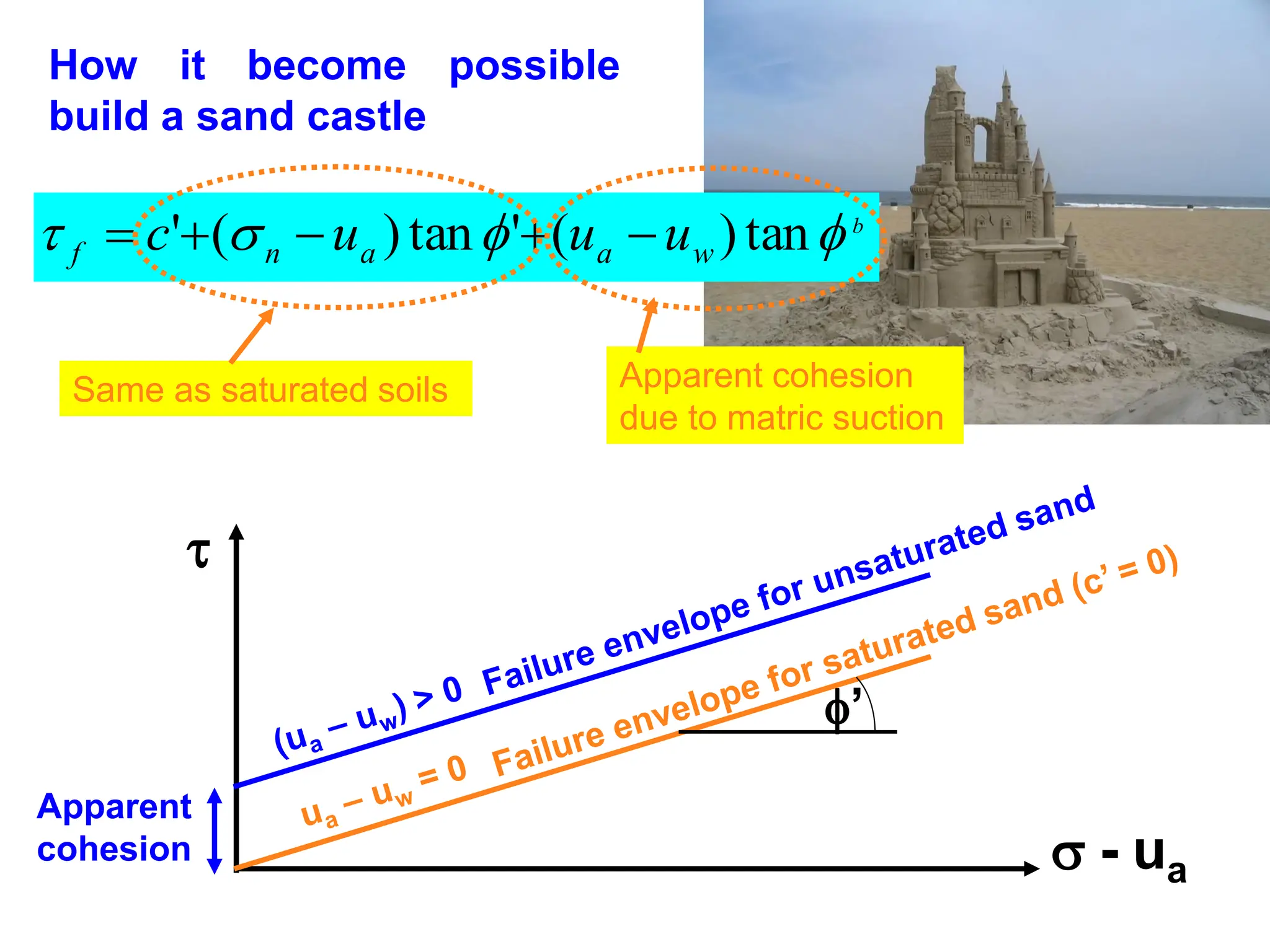
133.
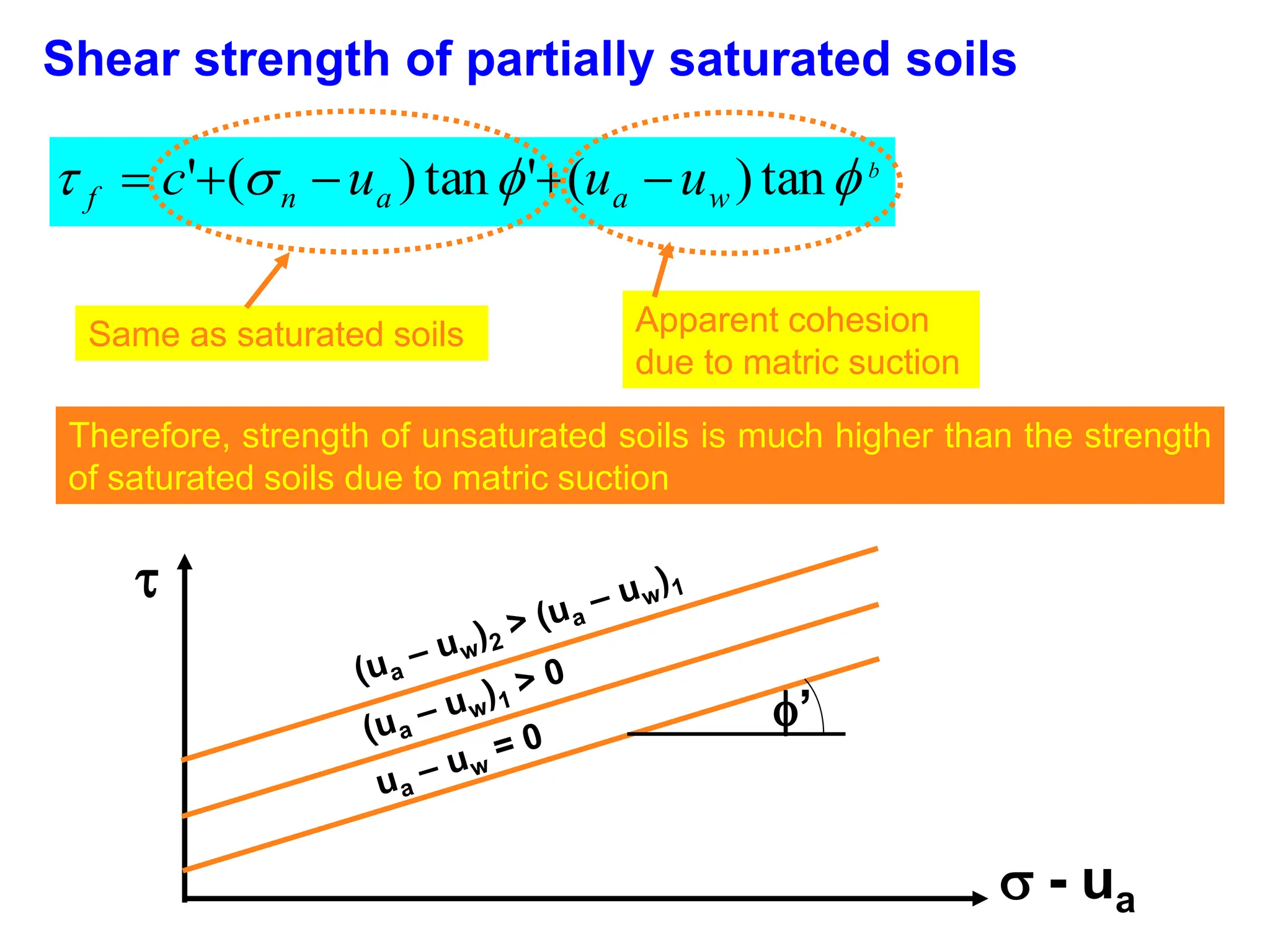
Shear strength ofpartially saturated soils
b
w
a
a
n
f u
u
u
c
tan
)
(
'
tan
)
(
'
Same as saturated soils Apparent cohesion
due to matric suction
Therefore, strength of unsaturated soils is much higher than the strength
of saturated soils due to matric suction
- ua
’
134.
- ua
Howit become possible
build a sand castle
b
w
a
a
n
f u
u
u
c
tan
)
(
'
tan
)
(
'
Same as saturated soils Apparent cohesion
due to matric suction
’
Apparent
cohesion


![Unconsolidated- Undrained test (UU Test)
Combining steps 2 and 3,
uc = B 3 ud = ABd
u = uc + ud
Total pore water pressure increment at any stage, u
u = B [3 + Ad]
Skempton’s pore
water pressure
equation
u = B [3 + A(1 – 3]](https://image.slidesharecdn.com/shearstrengthofsoil-251125083255-266fcb08/75/Shear-Strength-of-Soil-in-Geotechnical-engineering-pdf-73-2048.jpg)