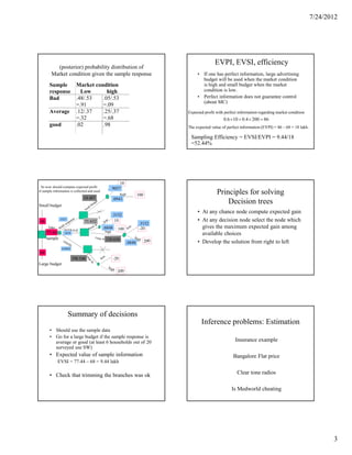
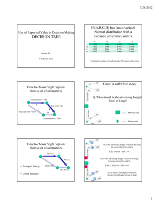
SlideShare a Scribd company logo
1 of 5
Download to read offline
7/24/2012


                                                                                If (A,B,C,D) has (multivariate)
Use of Expected Value in Decision Making                                           Normal distribution with a
               DECISION TREE                                                       variance covariance matrix
                                                                                    A                    B                C                D
                                                                            A     2.000                1.061           0.490            0.022
                                                                            B     1.061                1.000           0.043            0.158
                                                                            C     0.490                0.043           0.750            0.068
                                                                            D     0.022                0.158           0.068            0.100
                                 Session IX

                               A Softwhite story
                                                                                Calculate the chance of reaching under 16 hours in either route.


                                                                                           10
                                                                                                     Case: A softwhite story
         How to choose ‘right’ option
                                                                                           100
          from a set of alternatives
                                                                                     Q. What should be the advertising budget?
             Expected time = 10hr
                                                                                                 Small or Large?
                       A
                                                 Exp. Time 5 hr

                           C                 B
Expected time = 12hr                     D                                                                                            Decision node

                                    Expected time = 3.5hr
                                                                                                                                      Chance node


                                                                                           10
                                                                                .6
         How to choose ‘right’ option                                                                So, if the advertising budget is taken to be small,
                                                                                           100                  the expected profit would be
          from a set of alternatives                                             .4

                                                                                                             0.6 × 10 + 0.4 × 100 = 46
                                         N(10,2)

                                                                           46                    And, if the advertising budget is taken to be large,
                                                                  N(5,1)
                                                                                                            the expected profit would be

 • Example: lottery                   N(12,0.75)                                                       0.6 × (−20) + 0.4 × 200 = 68
                                                                           68
                                                            N(3.5,0.1)
                                                                                                          So, in absence of sample information,
 • Utility function                                                              .6
                                                                                                          the advertising budget should be large

                                                                                      .4


                                                                                                                                                               1
7/24/2012


                    10                                      10

                                                                       100                   P[‘LOW’ market condition given
                    100
                                                                 -20                          that sample response is BAD] ?
                                                                             200
                                       Large budget
                                                                                             P[market condition is low] = 0.6
         Take
                                                                                         P[BAD sample response given ‘LOW’ market condition]
        sample


                    10                                      10
                                                                                                                 Binomial Distribution
                                                                       100
                    100                                                            low       high
                                                                                      0.2        0.4    values
                                                                                    0.0115     0.0000             0   0.8042   0.1256   If the market condition is high
                                                                                    0.0576     0.0005             1
                                                                                    0.1369     0.0031             2
                                                                                                                                        (40% of the users will buy SW),
                                            L
                                                                                    0.2054     0.0123             3                     what is the chance of 8 out of
                                                                                    0.2182     0.0350             4
                                                                                    0.1746     0.0746             5                     the 20 randomly chosen HH
         Take
                                                                                    0.1091     0.1244             6   0.1932   0.6297   purchasing SW?
                                                                                    0.0545     0.1659             7
                                                                                    0.0222     0.1797             8
                                                                                    0.0074     0.1597             9
                                                                                                                                            20
        sample                                                                      0.0020     0.1171            10   0.0026   0.2447            C 8 ×0.408 × 0.6012 = 0.1797
                                                                                    0.0005     0.0710            11
                                                                                    0.0001     0.0355            12
                                                                                    0.0000     0.0146            13
                                                                                    0.0000     0.0049            14
                                                                                    0.0000     0.0013            15
                                                                                    0.0000     0.0003            16
                                                                                    0.0000     0.0000            17
                                                                                    0.0000     0.0000            18
                                                                                    0.0000     0.0000            19
                                                                                    0.0000     0.0000            20


                                                            10
     So now should compute expected profit            .6?                                Probability through Venn Diagram
   if sample information is collected and used
                                                                       100
                                                                                                                                                        0.4 ×1256=0.05
Small budget

                                            L
   46                                                                                                            0.60×.8042=0.48
                                                                                         BAD                                                              0.25
         Take
                                                                                                                                                         AVERAGE
        sample

                                                                                                                                                                 0.10
   68                                                                                                        0.60 ×0.1932=0.12
                                                                                                                                                       GOOD
 Large budget
                                                                                                                      Low                                        High


                                                                                                                                                                                       2
7/24/2012


                                                                                            EVPI, EVSI, efficiency
          (posterior) probability distribution of
        Market condition given the sample response                                • If one has perfect information, large advertising
                                                                                    budget will be used when the market condition
       Sample              Market condition                                         is high and small budget when the market
       response              Low       high                                         condition is low.
       Bad                 .48/.53   .05/.53                                      • Perfect information does not guarantee control
                                                                                    (about MC)
                           =.91      =.09
       Average             .12/.37   .25/.37                                 Expected profit with perfect information regarding market condition
                           =.32      =.68                                                        0.6 × 10 + 0.4 × 200 = 86
       good                .02       .98                                     The expected value of perfect information (EVPI) = 86 – 68 = 18 lakh..

                                                                              Sampling Efficiency = EVSI/EVPI = 9.44/18
                                                                              =52.44%


                                                       10
  So now should compute expected profit          . 9057
if sample information is collected and used
                                                                    100                      Principles for solving
                               18.487             .0943
Small budget
                                                                                                 Decision trees
                                                                                  • At any chance node compute expected gain
                                                  .3152
                                         L
46
              .5327
                                71.632                                            • At any decision node select the node which
                                                                     .3152
      Take                                    .6848                                 gives the maximum expected gain among
     77.44       .3678                                                              available choices
     sample                                    130.656
                                                            .6848                 • Develop the solution from right to left
                0.0994
68
                         196.546
Large budget


                      Summary of decisions
                                                                                    Inference problems: Estimation
       • Should use the sample data
       • Go for a large budget if the sample response is
         average or good (at least 6 households out of 20                                               Insurance example
         surveyed use SW)
       • Expected value of sample information                                                          Bangalore Flat price
             EVSI = 77.44 – 68 = 9.44 lakh

       • Check that trimming the branches was ok                                                         Clear tone radios

                                                                                                      Is Medworld cheating


                                                                                                                                                          3
7/24/2012


             A simple example: Overview
                                                                                                    Parameter &                           Statistic
  Population = all projects undertaken by a company
  An unknown proportion π of them took longer than scheduled
                                                                                            • A characteristic of the            • A characteristic of the
                                            *                                                 population which is of
   * Delay                                             *                                                                           sample (to estimate
                                 *        * *                          *                      interest in the study
                                           **             *                                                                        the parameter)
                             *              *                                               • Fixed or Non-random
                                     *    *           *                                                                          • Random (because the
                                                              **
                             *            * *         *                    *                                                       sample is random)
                                                                                            • Unknown (because
                                                                                              typically you don’t have           • Computable or
A random sample of n projects are selected. Y of them are found to be delayed.
                                                                                              information about all units          known once you draw
  (sample outcome) Y is random, but the randomness depends on π.                              of the population)                   the sample

  Given the value of Y, one can make an objective inference about π.


                                                                                                   Estimator/Estimate and
             Some of the questions to be
                                                                                               its Bias, Standard Error and
                     answered
                                                                                                   Sampling Distribution
      • To what degree, the randomness in Y can be
                                                                                            • Value of the Estimator (statistic) for a given
        attributed to sampling fluctuations?                                                  sample is your estimate
      • How close is Y = p to π ?                                                           • Bias = Mean (expected value) of the Estimator
                       n
      • If we want p to be within ±0.05 of π , how                                            minus the parameter
        many projects do we need to look at?                                                • Standard Error = Standard deviation of the
                                                                                              Estimator
                                                                                            • Sampling Distribution is the probability
                                                                                              distribution of the Estimator

                                                                                                                                                                 24


                                                                                                  Simple Random Sampling
                       º         º                                º            ×                           (SRS)
                                         ×        º                                         • Each unit in the population has equal chance of being
                 ×                                                ××           ×              included in the sample (even position-wise in the sample)
                 º                   ××
                         º                º                                                 • SRS with replacement (SRSWR): unit already selected are
                   ××                                                                  º      returned before drawing subsequent ones. (Same unit may
                     ×                     ×××
                       ×                                                                ×     appear more than once). Not too realistic but most useful
                                                              º                               for theoretical treatment
  N = 50                                 ×× º
                                 º                                                          • SRS without replacement (SRSWOR):
  n=5
                   º                                                                           – same unit may not be included more than once
                                 ×            º
                                                                                               – selections are not independent
                                                                                   º           – if the population size is very large compared to sample size,
                                                              ×
                                                                                                 SRSWOR can be considered/approximated by SRSWR


          Parameter (θ) = proportion of ‘×’ in the population


                                                                                                                                                                             4
7/24/2012


    Unbiasedness and Standard error
      of Sample Mean/Proportion
E( X ) = µ          E ( p) = π
               σ                   π (1 − π )
S .E.( X ) =        S .E.( p ) =
            n                          n
Estimated standard errors:
               S                   p (1 − p )
S .E.( X ) =        S .E.( p ) =
                n                      n26


                                                       5

More Related Content

Viewers also liked

median and order statistics
median and order statisticsmedian and order statistics
median and order statisticsShashank Singh
 
Next higher number with same number of binary bits set
Next higher number with same number of binary bits setNext higher number with same number of binary bits set
Next higher number with same number of binary bits setGowriKumar Chandramouli
 
Medians and Order Statistics
Medians and Order StatisticsMedians and Order Statistics
Medians and Order StatisticsHoa Nguyen
 
07 Analysis of Algorithms: Order Statistics
07 Analysis of Algorithms: Order Statistics07 Analysis of Algorithms: Order Statistics
07 Analysis of Algorithms: Order StatisticsAndres Mendez-Vazquez
 
Algorithm Design and Complexity - Course 8
Algorithm Design and Complexity - Course 8Algorithm Design and Complexity - Course 8
Algorithm Design and Complexity - Course 8Traian Rebedea
 

Viewers also liked (6)

median and order statistics
median and order statisticsmedian and order statistics
median and order statistics
 
Sufficient statistics
Sufficient statisticsSufficient statistics
Sufficient statistics
 
Next higher number with same number of binary bits set
Next higher number with same number of binary bits setNext higher number with same number of binary bits set
Next higher number with same number of binary bits set
 
Medians and Order Statistics
Medians and Order StatisticsMedians and Order Statistics
Medians and Order Statistics
 
07 Analysis of Algorithms: Order Statistics
07 Analysis of Algorithms: Order Statistics07 Analysis of Algorithms: Order Statistics
07 Analysis of Algorithms: Order Statistics
 
Algorithm Design and Complexity - Course 8
Algorithm Design and Complexity - Course 8Algorithm Design and Complexity - Course 8
Algorithm Design and Complexity - Course 8
 

More from vivek_shaw

Lecture 11 market structure- perfect competition
Lecture 11  market structure- perfect competitionLecture 11  market structure- perfect competition
Lecture 11 market structure- perfect competitionvivek_shaw
 
Lecture 9 costs
Lecture 9  costsLecture 9  costs
Lecture 9 costsvivek_shaw
 
Lecture 8 production, optimal inputs
Lecture 8  production, optimal inputsLecture 8  production, optimal inputs
Lecture 8 production, optimal inputsvivek_shaw
 
Lecture 8 production, optimal inputs (1)
Lecture 8  production, optimal inputs (1)Lecture 8  production, optimal inputs (1)
Lecture 8 production, optimal inputs (1)vivek_shaw
 
Lecture 3 dds sand elasticity
Lecture 3  dds sand elasticityLecture 3  dds sand elasticity
Lecture 3 dds sand elasticityvivek_shaw
 
Consumertheory1
Consumertheory1Consumertheory1
Consumertheory1vivek_shaw
 
Consumer theory 2
Consumer theory 2Consumer theory 2
Consumer theory 2vivek_shaw
 
Class2 market, demand and supply
Class2  market, demand and supplyClass2  market, demand and supply
Class2 market, demand and supplyvivek_shaw
 
Policy implications
Policy implicationsPolicy implications
Policy implicationsvivek_shaw
 
Man org session 3-org and technology_5th july 2012
Man org session 3-org and technology_5th july 2012Man org session 3-org and technology_5th july 2012
Man org session 3-org and technology_5th july 2012vivek_shaw
 
Man org session 14_org decision making_16th august 2012
Man org session 14_org decision making_16th august 2012Man org session 14_org decision making_16th august 2012
Man org session 14_org decision making_16th august 2012vivek_shaw
 
Man org session 12_org learning_3rd august 2012
Man org session 12_org learning_3rd august 2012Man org session 12_org learning_3rd august 2012
Man org session 12_org learning_3rd august 2012vivek_shaw
 
Man org session 11 interorganizational relationships_2nd august 2012
Man org session 11 interorganizational relationships_2nd august 2012Man org session 11 interorganizational relationships_2nd august 2012
Man org session 11 interorganizational relationships_2nd august 2012vivek_shaw
 
Man org session 10_org control_27th july 2012
Man org session 10_org control_27th july 2012Man org session 10_org control_27th july 2012
Man org session 10_org control_27th july 2012vivek_shaw
 

More from vivek_shaw (20)

Lecture 11 market structure- perfect competition
Lecture 11  market structure- perfect competitionLecture 11  market structure- perfect competition
Lecture 11 market structure- perfect competition
 
Lecture 9 costs
Lecture 9  costsLecture 9  costs
Lecture 9 costs
 
Lecture 8 production, optimal inputs
Lecture 8  production, optimal inputsLecture 8  production, optimal inputs
Lecture 8 production, optimal inputs
 
Lecture 8 production, optimal inputs (1)
Lecture 8  production, optimal inputs (1)Lecture 8  production, optimal inputs (1)
Lecture 8 production, optimal inputs (1)
 
Lecture 3 dds sand elasticity
Lecture 3  dds sand elasticityLecture 3  dds sand elasticity
Lecture 3 dds sand elasticity
 
Game theory 3
Game theory 3Game theory 3
Game theory 3
 
Game theory 1
Game theory 1Game theory 1
Game theory 1
 
Game theory 2
Game theory 2Game theory 2
Game theory 2
 
Ford motors
Ford motorsFord motors
Ford motors
 
Consumertheory1
Consumertheory1Consumertheory1
Consumertheory1
 
Consumer theory 2
Consumer theory 2Consumer theory 2
Consumer theory 2
 
Class2 market, demand and supply
Class2  market, demand and supplyClass2  market, demand and supply
Class2 market, demand and supply
 
Auctions 1
Auctions 1Auctions 1
Auctions 1
 
Costs2
Costs2Costs2
Costs2
 
Policy implications
Policy implicationsPolicy implications
Policy implications
 
Man org session 3-org and technology_5th july 2012
Man org session 3-org and technology_5th july 2012Man org session 3-org and technology_5th july 2012
Man org session 3-org and technology_5th july 2012
 
Man org session 14_org decision making_16th august 2012
Man org session 14_org decision making_16th august 2012Man org session 14_org decision making_16th august 2012
Man org session 14_org decision making_16th august 2012
 
Man org session 12_org learning_3rd august 2012
Man org session 12_org learning_3rd august 2012Man org session 12_org learning_3rd august 2012
Man org session 12_org learning_3rd august 2012
 
Man org session 11 interorganizational relationships_2nd august 2012
Man org session 11 interorganizational relationships_2nd august 2012Man org session 11 interorganizational relationships_2nd august 2012
Man org session 11 interorganizational relationships_2nd august 2012
 
Man org session 10_org control_27th july 2012
Man org session 10_org control_27th july 2012Man org session 10_org control_27th july 2012
Man org session 10_org control_27th july 2012
 

Session 9 10

  • 1. 7/24/2012 If (A,B,C,D) has (multivariate) Use of Expected Value in Decision Making Normal distribution with a DECISION TREE variance covariance matrix A B C D A 2.000 1.061 0.490 0.022 B 1.061 1.000 0.043 0.158 C 0.490 0.043 0.750 0.068 D 0.022 0.158 0.068 0.100 Session IX A Softwhite story Calculate the chance of reaching under 16 hours in either route. 10 Case: A softwhite story How to choose ‘right’ option 100 from a set of alternatives Q. What should be the advertising budget? Expected time = 10hr Small or Large? A Exp. Time 5 hr C B Expected time = 12hr D Decision node Expected time = 3.5hr Chance node 10 .6 How to choose ‘right’ option So, if the advertising budget is taken to be small, 100 the expected profit would be from a set of alternatives .4 0.6 × 10 + 0.4 × 100 = 46 N(10,2) 46 And, if the advertising budget is taken to be large, N(5,1) the expected profit would be • Example: lottery N(12,0.75) 0.6 × (−20) + 0.4 × 200 = 68 68 N(3.5,0.1) So, in absence of sample information, • Utility function .6 the advertising budget should be large .4 1
  • 2. 7/24/2012 10 10 100 P[‘LOW’ market condition given 100 -20 that sample response is BAD] ? 200 Large budget P[market condition is low] = 0.6 Take P[BAD sample response given ‘LOW’ market condition] sample 10 10 Binomial Distribution 100 100 low high 0.2 0.4 values 0.0115 0.0000 0 0.8042 0.1256 If the market condition is high 0.0576 0.0005 1 0.1369 0.0031 2 (40% of the users will buy SW), L 0.2054 0.0123 3 what is the chance of 8 out of 0.2182 0.0350 4 0.1746 0.0746 5 the 20 randomly chosen HH Take 0.1091 0.1244 6 0.1932 0.6297 purchasing SW? 0.0545 0.1659 7 0.0222 0.1797 8 0.0074 0.1597 9 20 sample 0.0020 0.1171 10 0.0026 0.2447 C 8 ×0.408 × 0.6012 = 0.1797 0.0005 0.0710 11 0.0001 0.0355 12 0.0000 0.0146 13 0.0000 0.0049 14 0.0000 0.0013 15 0.0000 0.0003 16 0.0000 0.0000 17 0.0000 0.0000 18 0.0000 0.0000 19 0.0000 0.0000 20 10 So now should compute expected profit .6? Probability through Venn Diagram if sample information is collected and used 100 0.4 ×1256=0.05 Small budget L 46 0.60×.8042=0.48 BAD 0.25 Take AVERAGE sample 0.10 68 0.60 ×0.1932=0.12 GOOD Large budget Low High 2
  • 3. 7/24/2012 EVPI, EVSI, efficiency (posterior) probability distribution of Market condition given the sample response • If one has perfect information, large advertising budget will be used when the market condition Sample Market condition is high and small budget when the market response Low high condition is low. Bad .48/.53 .05/.53 • Perfect information does not guarantee control (about MC) =.91 =.09 Average .12/.37 .25/.37 Expected profit with perfect information regarding market condition =.32 =.68 0.6 × 10 + 0.4 × 200 = 86 good .02 .98 The expected value of perfect information (EVPI) = 86 – 68 = 18 lakh.. Sampling Efficiency = EVSI/EVPI = 9.44/18 =52.44% 10 So now should compute expected profit . 9057 if sample information is collected and used 100 Principles for solving 18.487 .0943 Small budget Decision trees • At any chance node compute expected gain .3152 L 46 .5327 71.632 • At any decision node select the node which .3152 Take .6848 gives the maximum expected gain among 77.44 .3678 available choices sample 130.656 .6848 • Develop the solution from right to left 0.0994 68 196.546 Large budget Summary of decisions Inference problems: Estimation • Should use the sample data • Go for a large budget if the sample response is average or good (at least 6 households out of 20 Insurance example surveyed use SW) • Expected value of sample information Bangalore Flat price EVSI = 77.44 – 68 = 9.44 lakh • Check that trimming the branches was ok Clear tone radios Is Medworld cheating 3
  • 4. 7/24/2012 A simple example: Overview Parameter & Statistic Population = all projects undertaken by a company An unknown proportion π of them took longer than scheduled • A characteristic of the • A characteristic of the * population which is of * Delay * sample (to estimate * * * * interest in the study ** * the parameter) * * • Fixed or Non-random * * * • Random (because the ** * * * * * sample is random) • Unknown (because typically you don’t have • Computable or A random sample of n projects are selected. Y of them are found to be delayed. information about all units known once you draw (sample outcome) Y is random, but the randomness depends on π. of the population) the sample Given the value of Y, one can make an objective inference about π. Estimator/Estimate and Some of the questions to be its Bias, Standard Error and answered Sampling Distribution • To what degree, the randomness in Y can be • Value of the Estimator (statistic) for a given attributed to sampling fluctuations? sample is your estimate • How close is Y = p to π ? • Bias = Mean (expected value) of the Estimator n • If we want p to be within ±0.05 of π , how minus the parameter many projects do we need to look at? • Standard Error = Standard deviation of the Estimator • Sampling Distribution is the probability distribution of the Estimator 24 Simple Random Sampling º º º × (SRS) × º • Each unit in the population has equal chance of being × ×× × included in the sample (even position-wise in the sample) º ×× º º • SRS with replacement (SRSWR): unit already selected are ×× º returned before drawing subsequent ones. (Same unit may × ××× × × appear more than once). Not too realistic but most useful º for theoretical treatment N = 50 ×× º º • SRS without replacement (SRSWOR): n=5 º – same unit may not be included more than once × º – selections are not independent º – if the population size is very large compared to sample size, × SRSWOR can be considered/approximated by SRSWR Parameter (θ) = proportion of ‘×’ in the population 4
  • 5. 7/24/2012 Unbiasedness and Standard error of Sample Mean/Proportion E( X ) = µ E ( p) = π σ π (1 − π ) S .E.( X ) = S .E.( p ) = n n Estimated standard errors: S p (1 − p ) S .E.( X ) = S .E.( p ) = n n26 5