Downloaded 135 times
![13
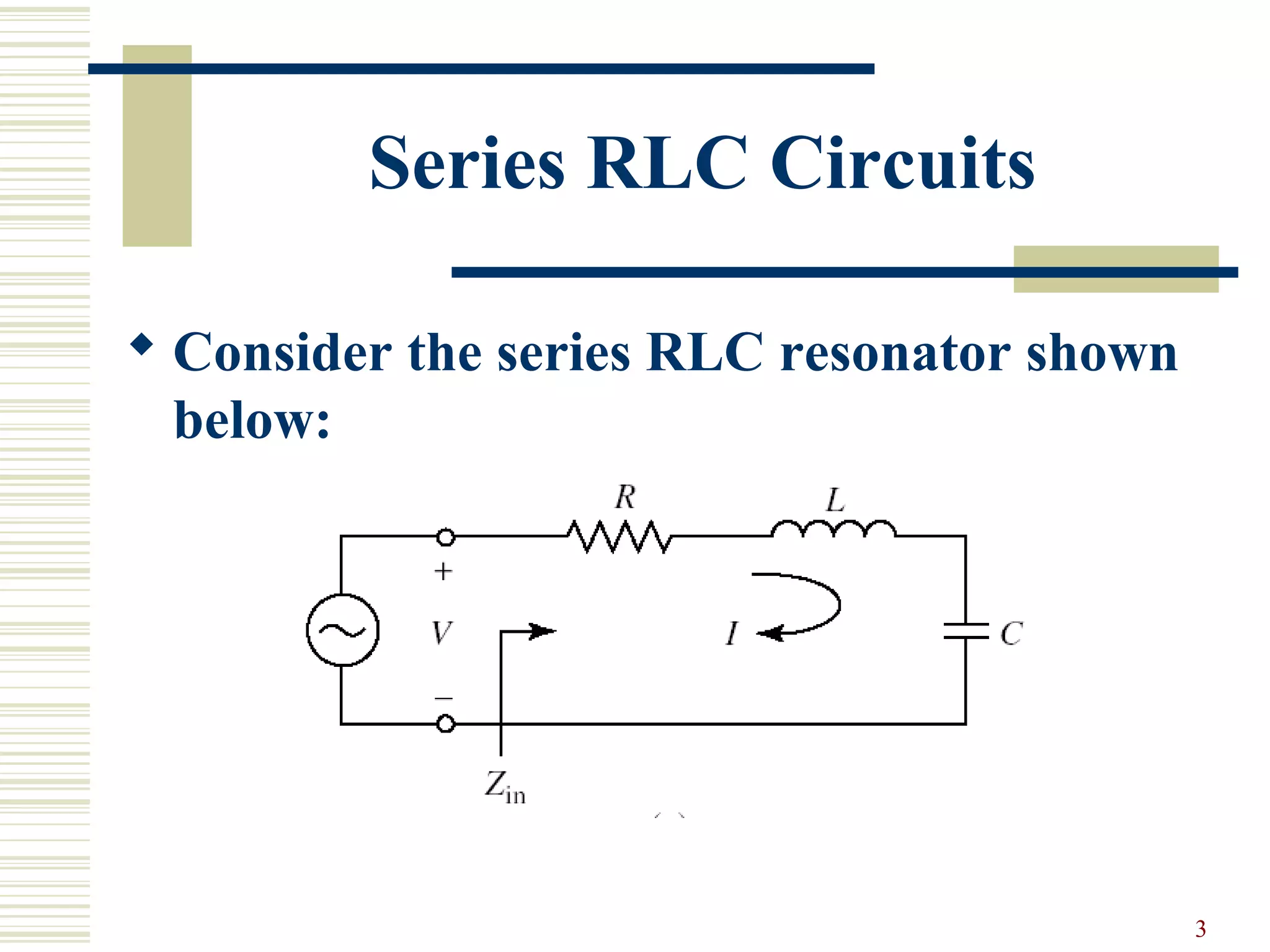
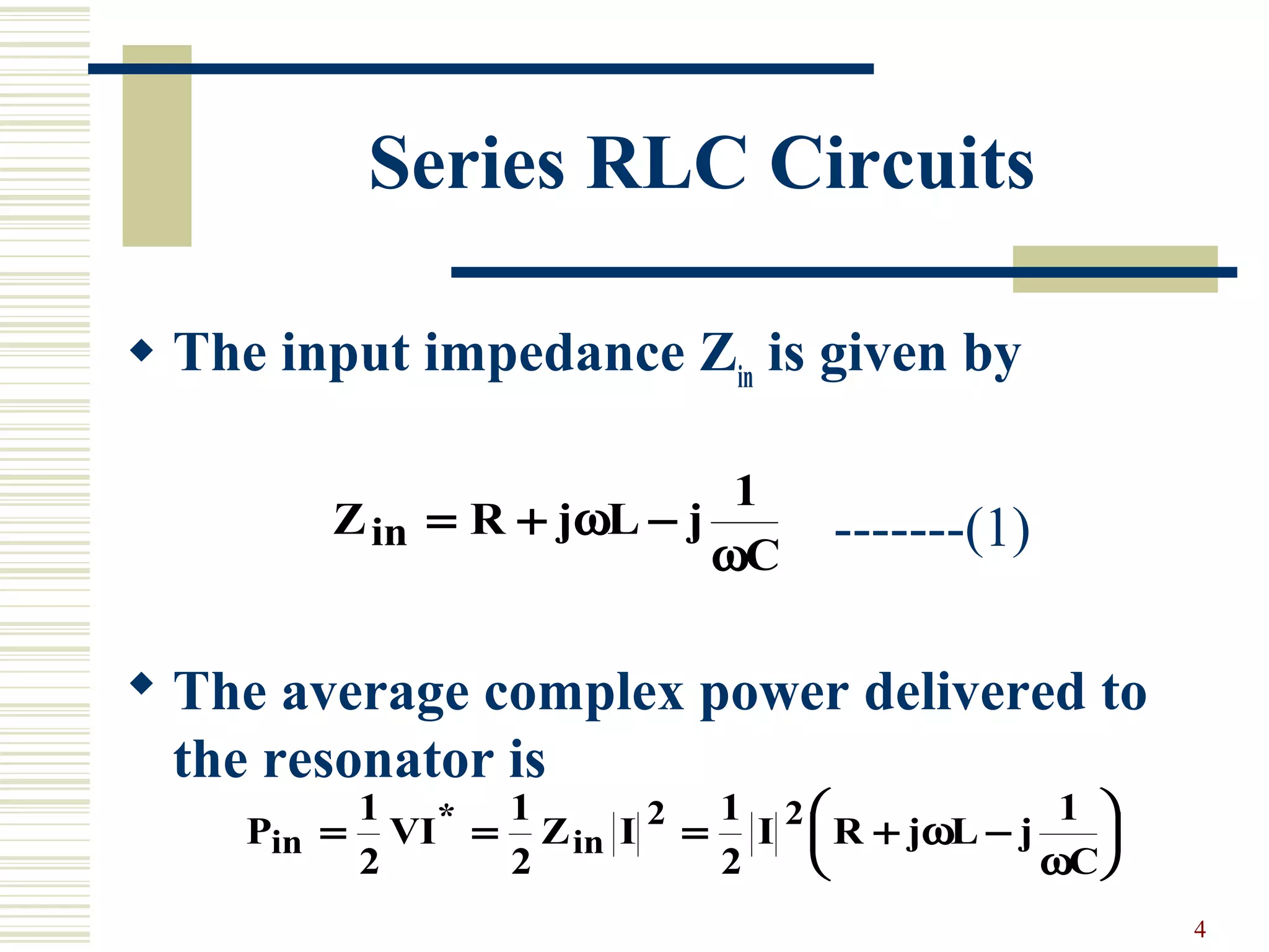
Series RLC Circuits
Consider the equation
As
---(5)
Z R j L
L
Q
j Lin
o
o≈ + = + −2 2∆ω
ω
ω ω( )
Q
L
R
o=
ω
Z j L
j Q
j L j
Q
in o
o
o≈ − + = − +2
2
2 1
1
2
( ) [ ( )]ω ω
ω
ω ω](https://image.slidesharecdn.com/seriesandparallelresonators-131002215027-phpapp01/75/Series-and-parallel-resonators-12-2048.jpg)
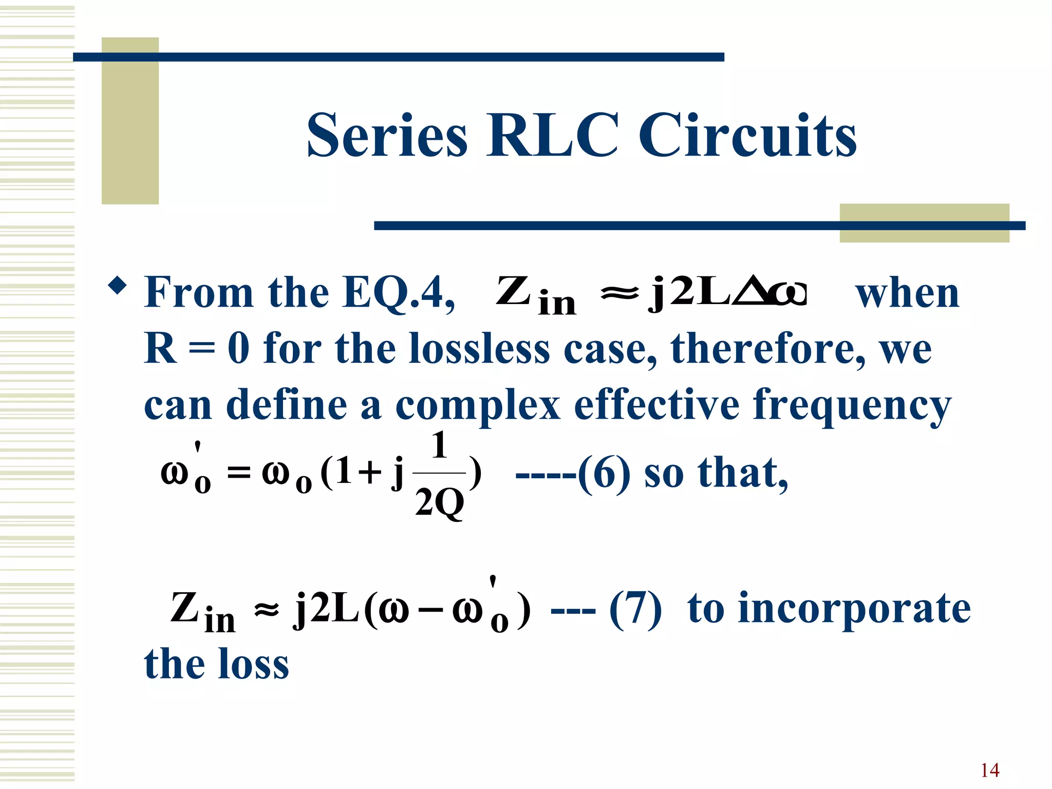
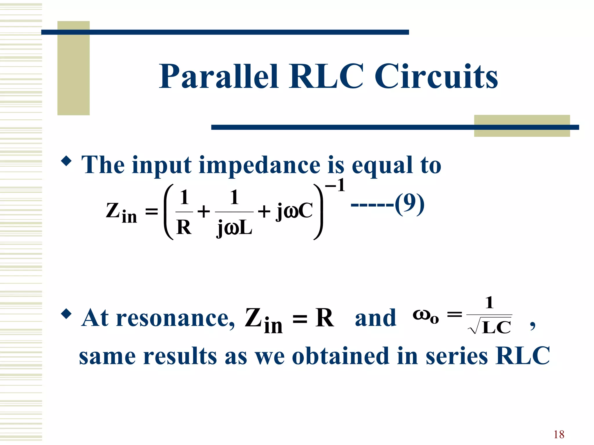
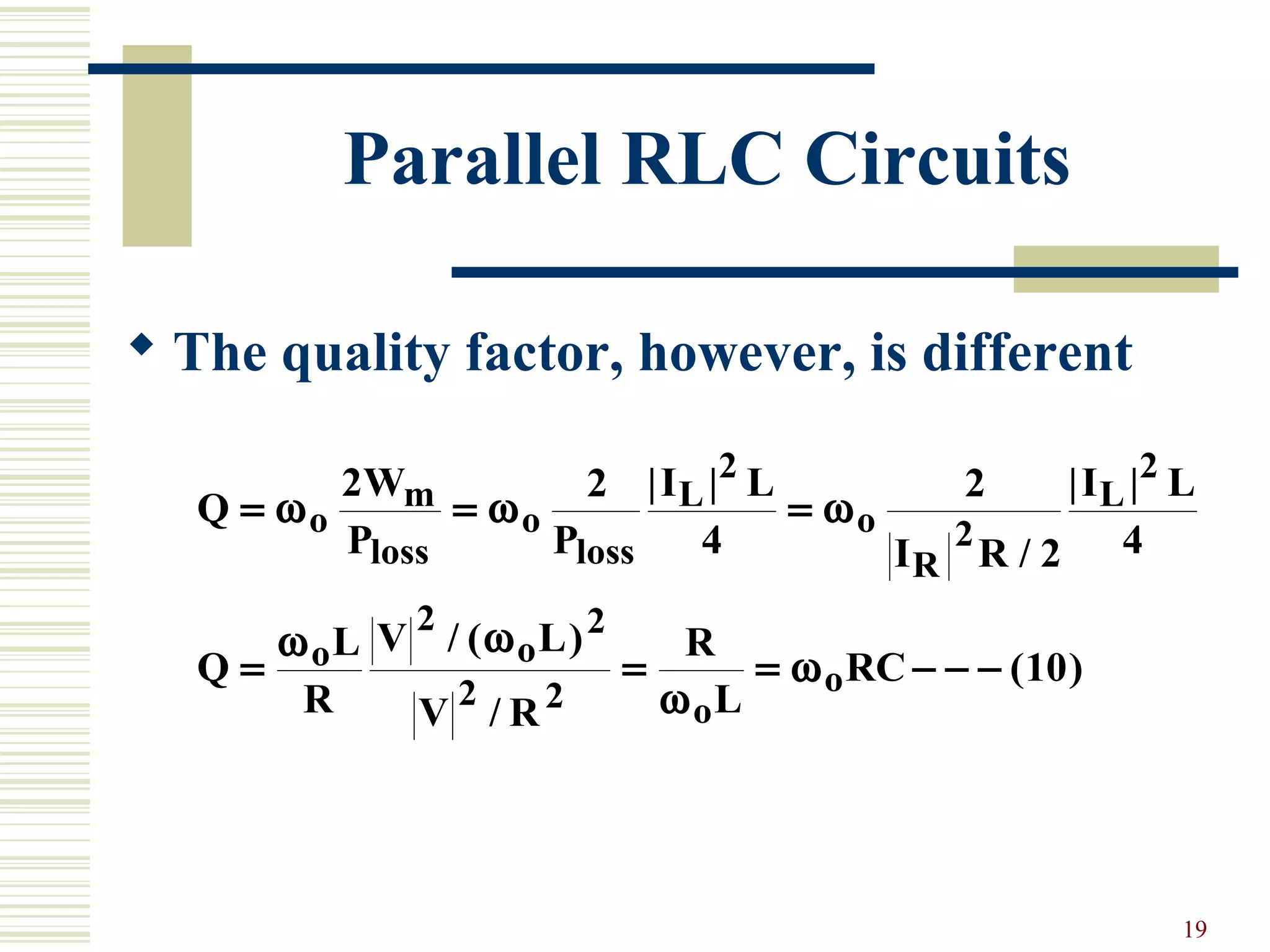
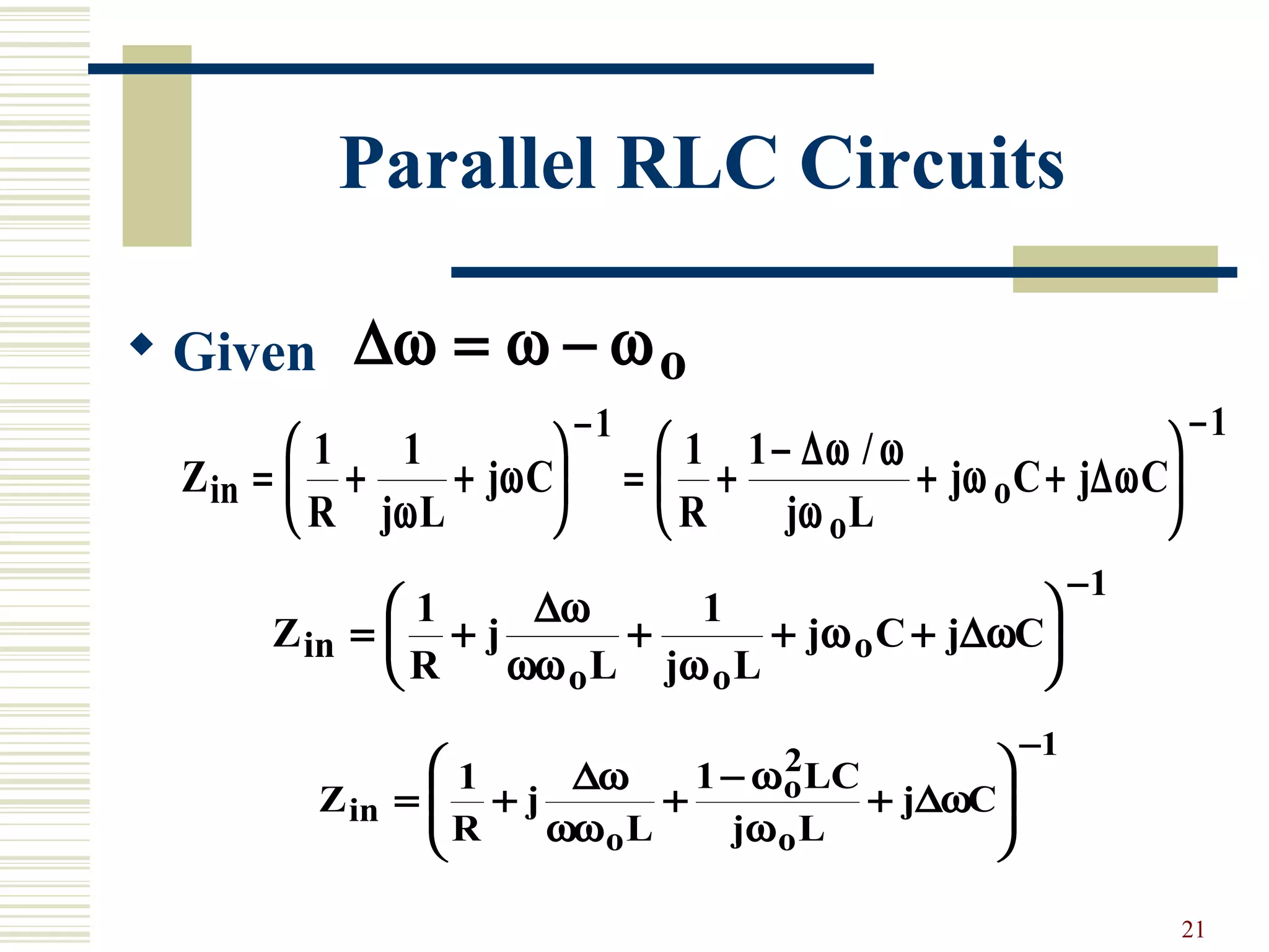
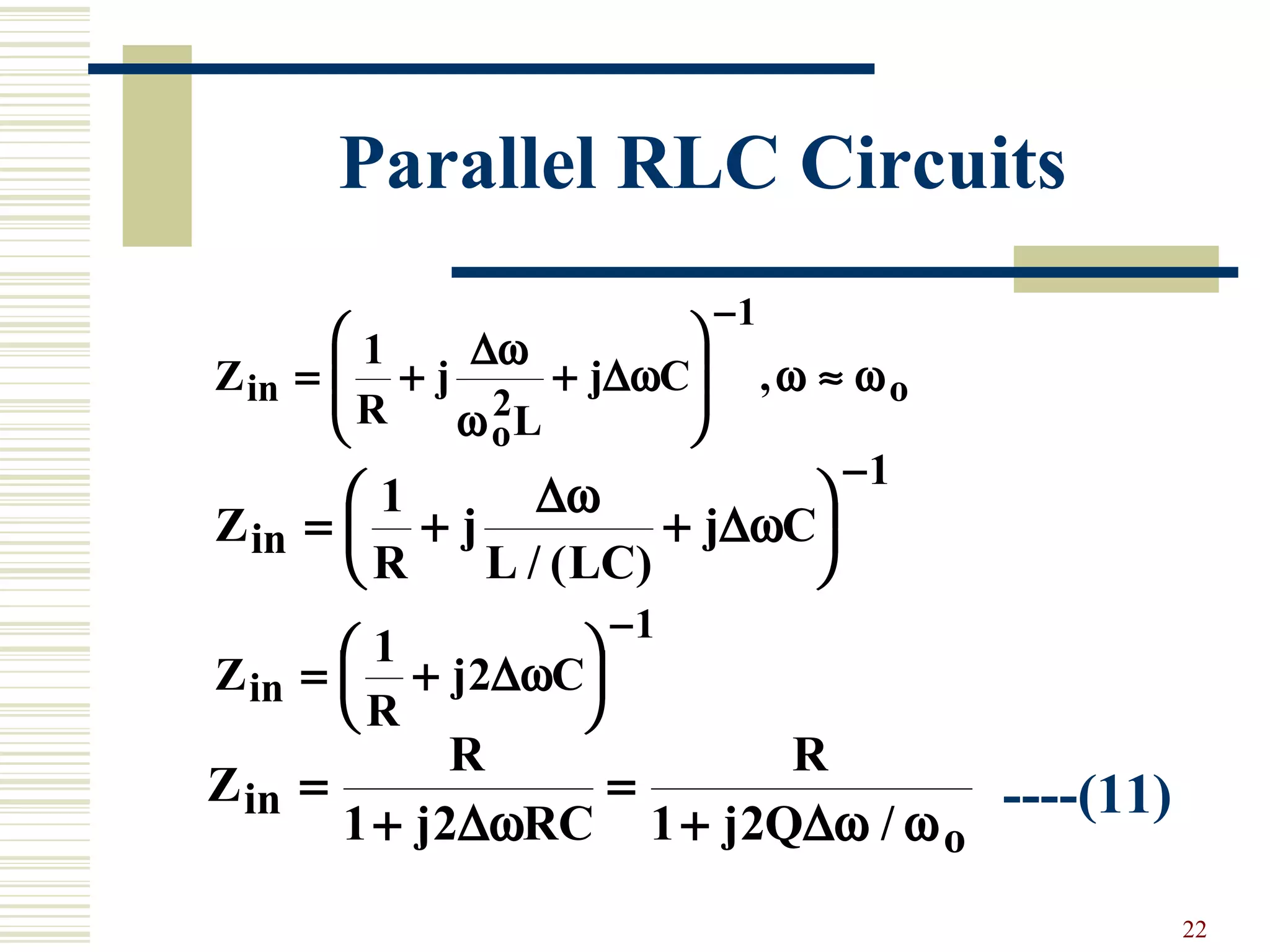
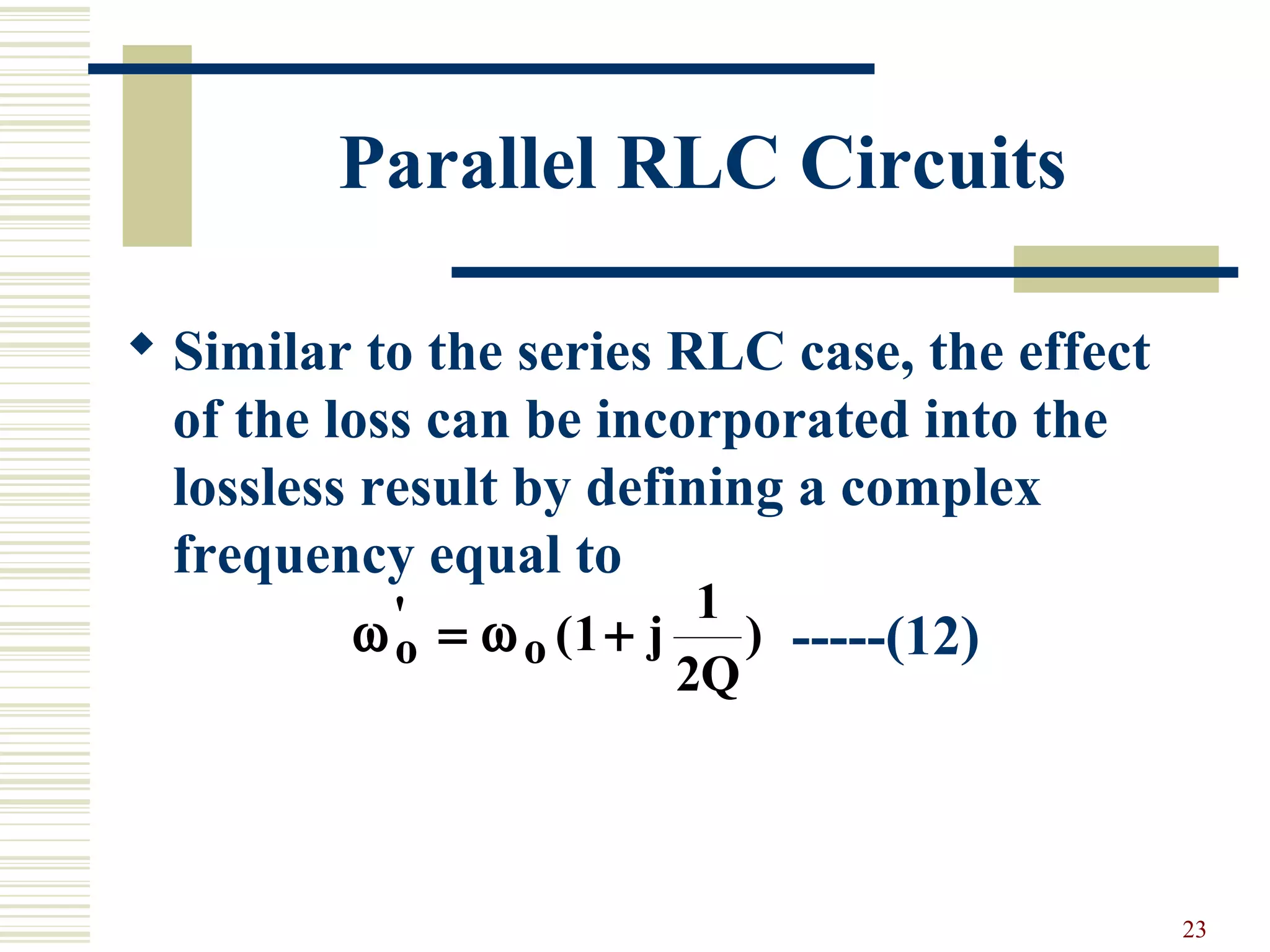
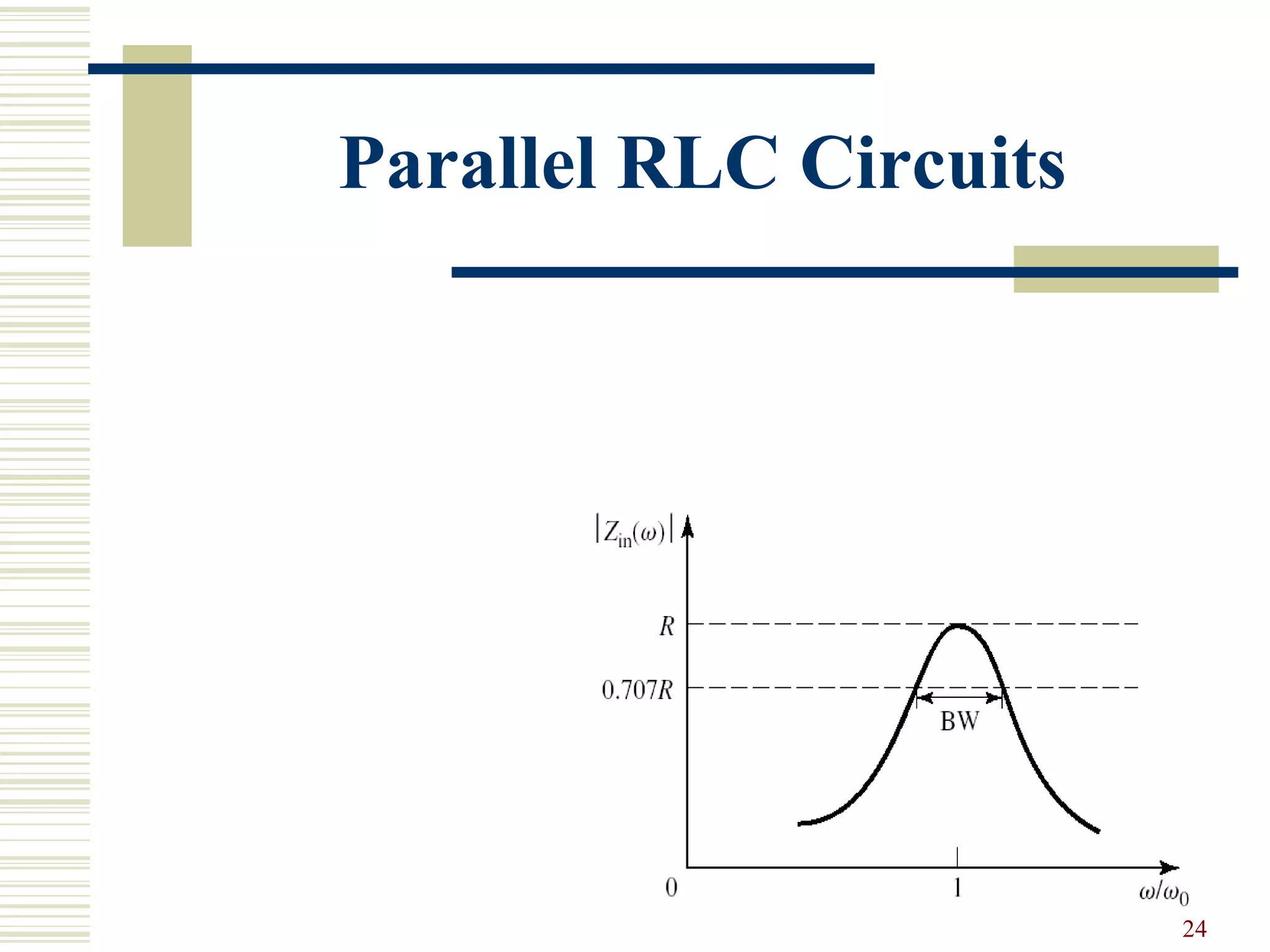
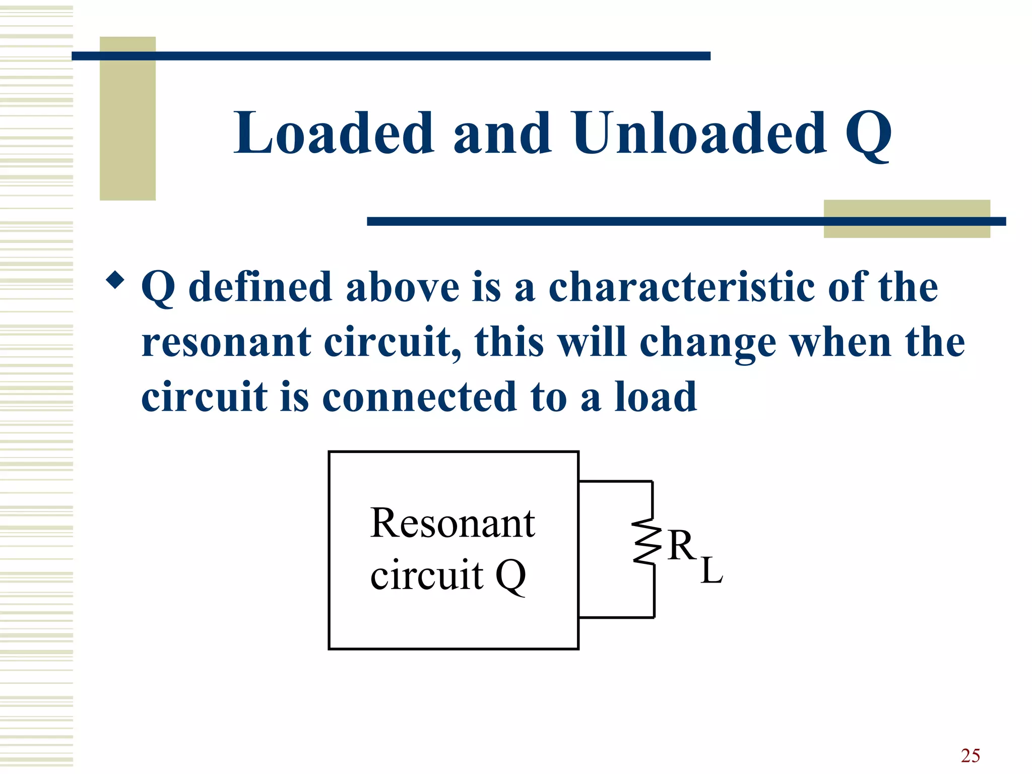
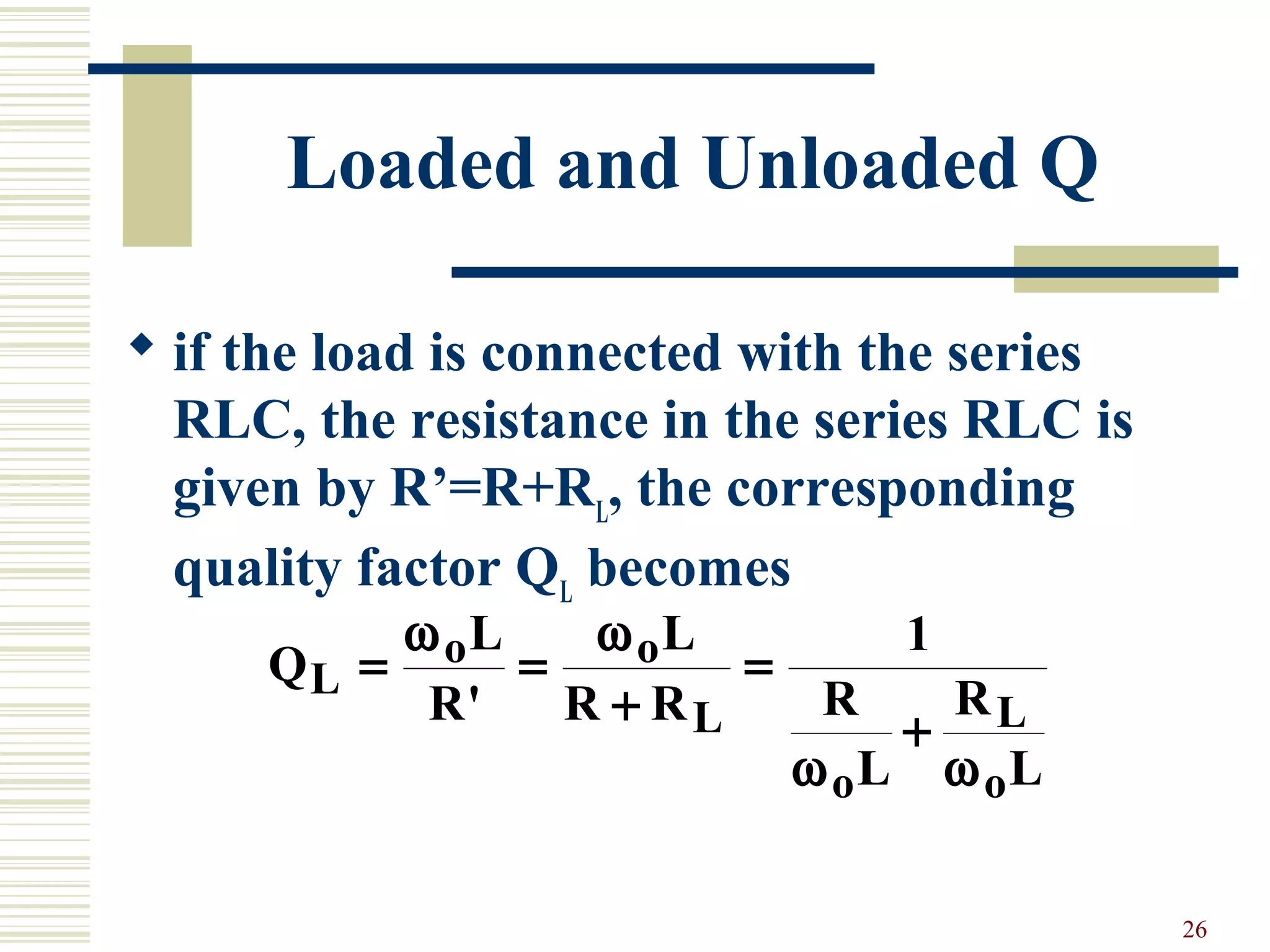
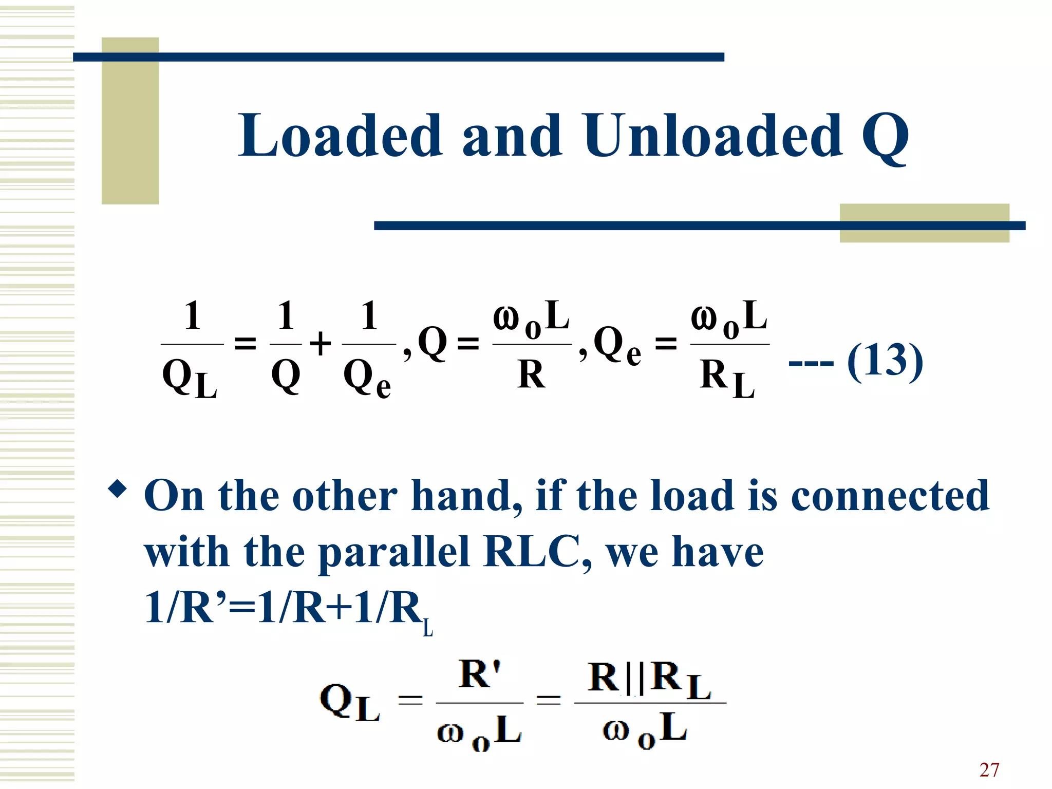
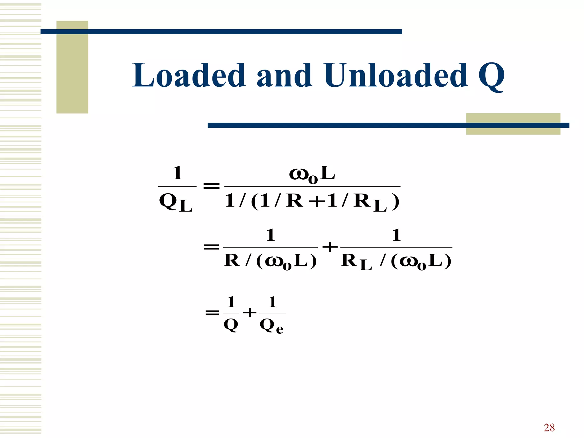
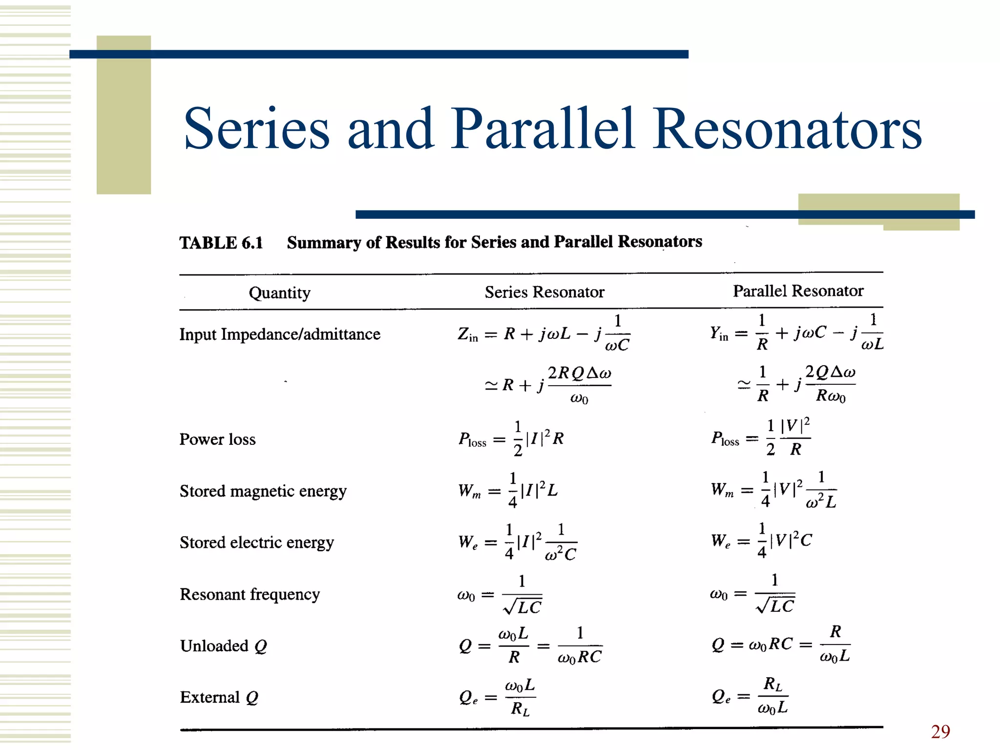


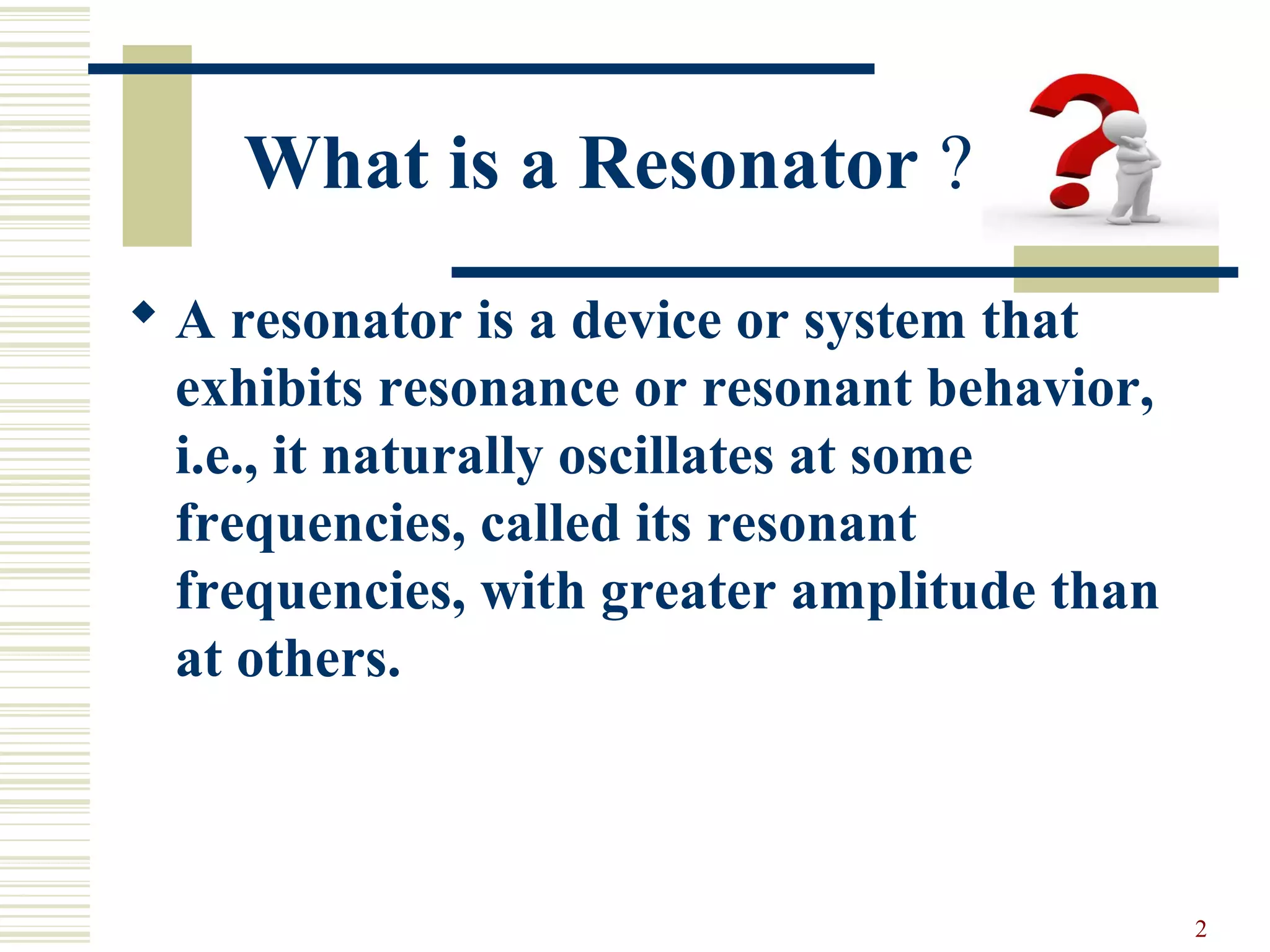
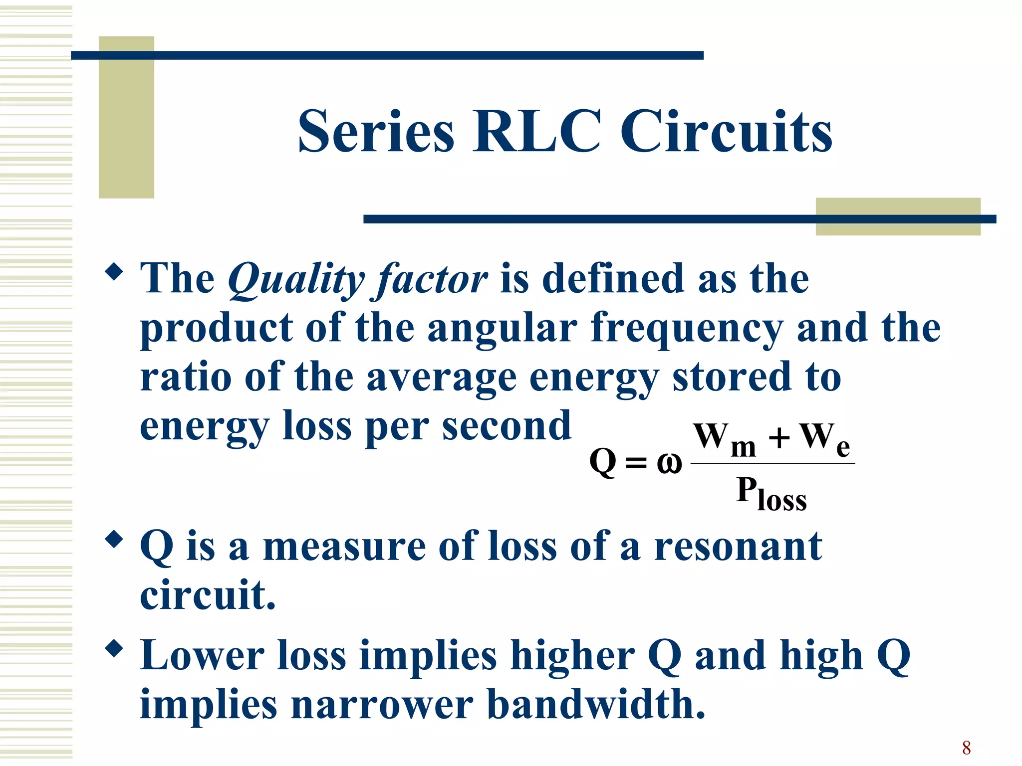
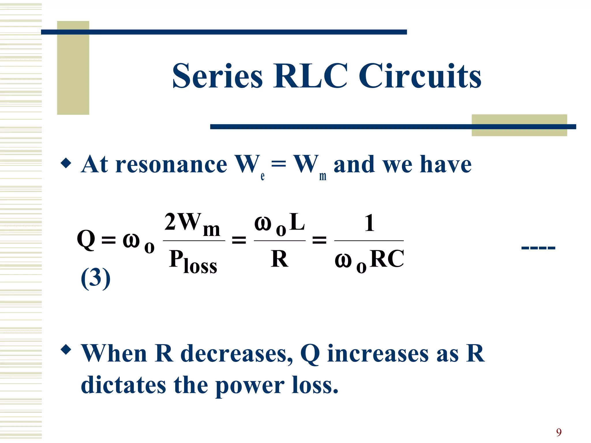
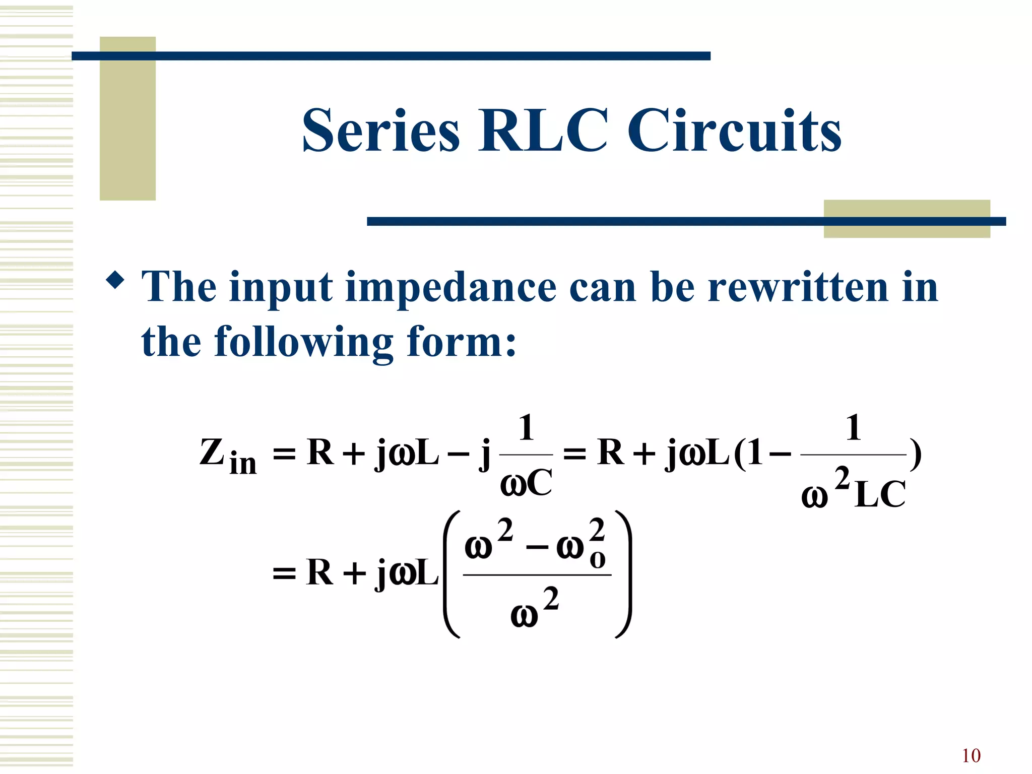
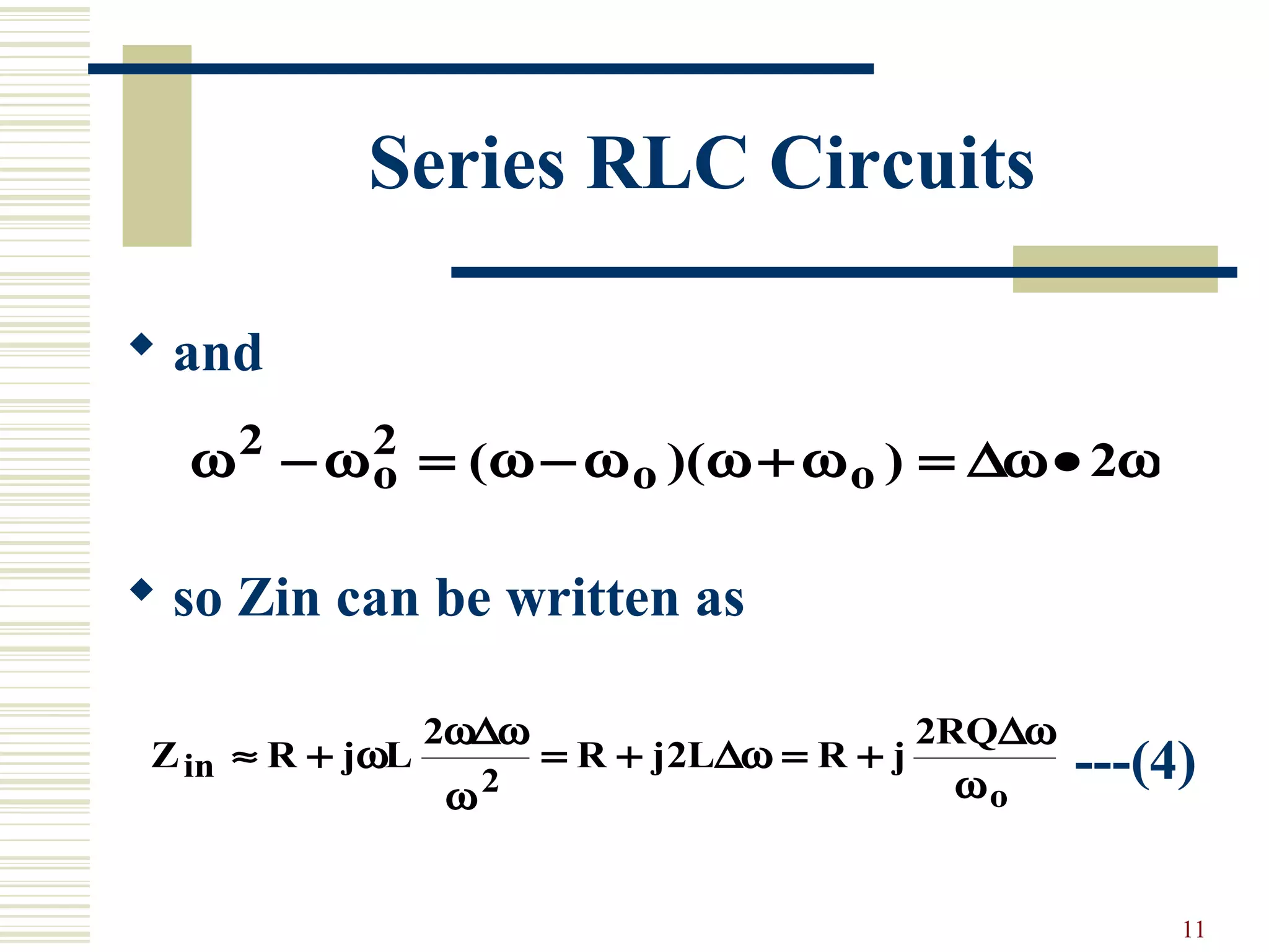
Series and parallel RLC resonator circuits are discussed. A series RLC circuit exhibits resonance at the angular frequency where the average stored magnetic energy equals the average stored electric energy. The quality factor Q of a series RLC circuit increases as the resistance R decreases. For a parallel RLC circuit, Q increases as R increases. Near resonance, the input impedance of both circuits can be approximated using Q and a complex effective frequency accounting for losses. The loaded Q of a resonant circuit decreases when connected to a resistive load.


![RF Circuit Design - [Ch4-1] Microwave Transistor Amplifier](https://cdn.slidesharecdn.com/ss_thumbnails/ch4-1-150613064409-lva1-app6892-thumbnail.jpg?width=640&height=640&fit=bounds)


![Digital Signal Processing[ECEG-3171]-Ch1_L02](https://cdn.slidesharecdn.com/ss_thumbnails/dspl2-180427094423-thumbnail.jpg?width=640&height=640&fit=bounds)