Separation Process Principles with Applications Using Process Simulators 4th Edition J. D. Seader
Separation Process Principles with Applications Using Process Simulators 4th Edition J. D. Seader
Separation Process Principles with Applications Using Process Simulators 4th Edition J. D. Seader


![Trim Size: 8.5in x 11in Seader f04.tex V2 - 10/16/2015 7:52 P.M. Page xx
xx Dimensions and Units
In the SI System, the prefix M, mega, stands for million. However, in the natural gas and petroleum industries of the United States, when
using the AE System, M stands for thousand and MM stands for million. Thus, MBtu stands for thousands of Btu, while MM Btu stands for
millions of Btu.
It should be noted that the common pressure and power units in use for the AE System are not consistent with the base units. Thus, for
pressure, pounds per square inch, psi or lbf/in.2
, is used rather than lbf/ft2
. For power, Hp is used instead of ft-lbf/h, where the conversion
factor is
1 hp = 1.980 × 10⁶
ft-lbf∕h
CONVERSION FACTORS
Physical constants may be found on the inside back cover of this book. Conversion factors are
given on the inside front cover. These factors permit direct conversion of AE and CGS values
to SI values. The following is an example of such a conversion, together with the reverse
conversion.
EXAMPLE
1. Convert 50 psia (lbf/in.2
absolute) to kPa:
The conversion factor for lbf/in.2
to Pa is 6,895, which results in
50(6, 895) = 345,000 Pa or 345 kPa
2. Convert 250 kPa to atm:
250 kPa = 250,000 Pa. The conversion factor for atm to Pa is 1.013 × 10⁵
. Therefore, dividing by the conversion factor,
250,000∕1.013 × 105
= 2.47 atm
Three of the units [gallons (gal), calories (cal), and British thermal unit (Btu)] in the list of conversion factors have two or more definitions.
The gallons unit cited here is the U.S. gallon, which is 83.3% of the Imperial gallon. The cal and Btu units used here are international (IT).
Also in common use are the thermochemical cal and Btu, which are 99.964% of the international cal and Btu.
FORMAT FOR EXERCISES IN THIS BOOK
In numerical exercises throughout this book, the system of units to be used to solve the problem
is stated. Then when given values are substituted into equations, units are not appended to the
values. Instead, the conversion of a given value to units in the above tables of base and derived
units is done prior to substitution into the equation or carried out directly in the equation, as
in the following example.
EXAMPLE
Using conversion factors on the inside back cover of this book, calculate a Reynolds number, NRe = Dvρ∕μ, given D = 4.0 ft, v = 4.5 ft∕s,
ρ = 60 lbm∕ft3
, and μ = 2.0 cP (i.e., centipoise).
Using the SI System (kg-m-s),
NRe =
Dvρ
μ
=
[(4.00)(0.3048)][(4.5)(0.3048)][(60)(16.02)]
[(2.0)(0.001)]
= 804,000
Using the CGS System (g-cm-s),
NRe =
Dvρ
μ
=
[(4.00)(30.48)][(4.5)(30.48)][(60)(0.01602)
[(0.02)]
= 804,000
Using the AE System (lbm-ft-h) and converting the viscosity 0.02 cP to lbm/ft-h,
NRe =
Dvρ
μ
=
(4.00)[(4.5)(3600)](60)
[(0.02)(241.9)]
= 804,000](https://image.slidesharecdn.com/79767-250509205929-f038e3ca/85/Separation-Process-Principles-with-Applications-Using-Process-Simulators-4th-Edition-J-D-Seader-27-320.jpg)


![Trim Size: 8.5in x 11in Seader c01.tex V2 - 10/16/2015 10:38 A.M. Page 3
§1.2 Basic Separation Techniques 3
Figure 1.3 Process for hydration of ethylene
to ethanol.
Figure 1.4 Industrial process for hydration of ethylene to ethanol.
Chemical engineers also design products that can involve
separation operations. One such product is the espresso coffee
machine. Very hot water rapidly leaches desirable chemicals
from the coffee bean, leaving behind ingredients responsible
for undesirable acidity and bitterness. The resulting cup of
espresso has (1) a topping of creamy foam that traps the
extracted chemicals, (2) a fullness of body due to emulsifica-
tion, and (3) a richness of aroma. Typically, 25% of the coffee
bean is extracted and the espresso contains less caffeine than
filtered coffee. Cussler and Moggridge [1] and Seider, Seader,
Lewin, and Widagdo [2] discuss other examples of products
designed by chemical engineers that involve the separation of
chemical mixtures.
§1.2 BASIC SEPARATION TECHNIQUES
The separation of a chemical mixture into its components is
not a spontaneous process, like the mixing by diffusion of
soluble components. Separations require energy in some form.
A mixture to be separated into its separate chemical species
is usually a single, homogeneous phase. If it is multiphase, it
is often best to first separate the phases by gravity or centrifu-
gation, followed by the separation of each phase mixture.
A schematic of a general separation process is shown in
Figure 1.5. The phase state of the feed can be a vapor, liquid,
or solid mixture. The products of the separation differ in
composition from the feed and may differ in the state of the](https://image.slidesharecdn.com/79767-250509205929-f038e3ca/85/Separation-Process-Principles-with-Applications-Using-Process-Simulators-4th-Edition-J-D-Seader-30-320.jpg)


![Trim Size: 8.5in x 11in Seader c01.tex V2 - 10/16/2015 10:38 A.M. Page 8
8 Chapter 1 Separation Processes
Until 1953, this process was the source of heavy water (D2O).
In electrodialysis, cation- and anion-permeable membranes
carry a fixed charge that prevents migration of species with like
charge. This phenomenon is applied to desalinate seawater. A
related process is electrophoresis, which exploits the different
migration velocities of charged colloidal or suspended species
in an electric field.
These external field separation operations are not discussed
further in this textbook, with the exception of electrodialysis,
which is described in Chapter 14.
§1.7 BRIEF COMPARISON OF COMMON
SEPARATION OPERATIONS
When selecting among feasible separation techniques for
a given application, some major factors to consider are
(1) technological maturity, which allows designers to apply
prior knowledge; (2) cost; (3) ease of scale-up from labora-
tory experiments; (4) ease of providing multiple stages; and
(5) need for parallel units for large capacities. A survey
by Keller [3], Figure 1.8, shows that the degree to which
a separation operation is technologically mature correlates
with its extent of commercial use. Operations based on mem-
branes are more expensive than those based on phase creation
(e.g., distillation) or phase addition (e.g., absorption, extrac-
tion, and adsorption). All separation equipment is limited
to a maximum size. For capacities requiring a larger size,
parallel units must be provided. Except for size constraints
or fabrication problems, capacity of a single unit can be dou-
bled for an additional investment cost of about 60%. If two
parallel units are installed, the additional investment for the
second unit is 100% of the first unit, unless a volume-discount
Technological maturity
Use
maturity
Distillation
Gas absorption
Ext./azeo. dist.
Solvent ext.
Crystallization
Ion exchange
Adsorption: gas feed
Membranes: gas feed
Membranes: liquid feed
Chromatography: liquid feed
Adsorption: liquid feed
Supercritical
gas abs./ext.
Liquid
membranes
Field-induced separations
Affinity separations
Invention Technology
asymptote
Use
asymptote
First
application
Figure 1.8 Technological and use maturities of separation
processes.
[Reproduced from [3] with permission of the American Institute of
Chemical Engineers.]
Table 1.4 Ease of Scale-Up of the Most Common Separations
Operation in Decreasing
Ease of Scale-Up
Ease of
Staging
Need for
Parallel Units
Distillation Easy No need
Absorption Easy No need
Liquid–liquid
extraction
Easy Sometimes
Membranes Re-pressurization
required between
stages
Almost always
Adsorption Easy Only for
regeneration
cycle
applies. Table 1.4 lists operations ranked according to ease of
scale-up. Those ranked near the top are frequently designed
without pilot-plant or laboratory data. Operations near the
middle usually require laboratory data, while those near
the bottom require pilot-plant tests. Included in the table is
an indication of the ease of providing multiple stages and
whether parallel units may be required. Ultimately, the most
cost-effective process, based on operating, maintenance, and
capital costs, is selected, provided it is controllable, safe,
and nonpolluting.
Also of interest are studies by Sherwood, Pigford, and
Wilke [4], Dwyer [5], and Keller [3] that show that the cost
of recovering and purifying a chemical depends strongly on
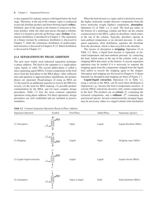
its concentration in the feed. Keller’s correlation, Figure 1.9,
shows that the more dilute the feed in the product, the higher
the product price. The five highest priced and most dilute
chemicals shown are all proteins.
Urokinase
Factor
VIII
Luciferase
Insulin
Rennin
Ag
Co
Hg
Ni
Cu
Zn
Citric
Acid
Penicillin
1,000,000,000
100,000,000
10,000,000
Price,
$/lb
Weight fraction in substrate
1,000,000
100,000
10,000
1,000
100
10
1 0.1 0.01 0.001
1
0.10
10–4
10–5
10–6
10–7
10–8
10–9
Figure 1.9 Effect of concentration of product in feed material on
price.
[Reproduced from [3] with permission of the American Institute of
Chemical Engineers.]](https://image.slidesharecdn.com/79767-250509205929-f038e3ca/85/Separation-Process-Principles-with-Applications-Using-Process-Simulators-4th-Edition-J-D-Seader-35-320.jpg)


![Trim Size: 8.5in x 11in Seader c01.tex V2 - 10/16/2015 10:38 A.M. Page 12
12 Chapter 1 Separation Processes
Table 1.7 Number of Alternative Sequences
Number of Final
Products
Number of
Columns
Number of Alternative
Sequences
2 1 1
3 2 2
4 3 5
5 4 14
6 5 42
4. Make the most difficult separations in the absence of the
other components. This will usually lower the diameter
of the tallest column.
5. Leave later in the sequence those separations that pro-
duce final products of the highest purities. This will also
lower the diameter of the tallest column.
6. Select the sequence that favors near-equimolar amounts
of distillate and bottoms in each column. Then the
two sections of the column will tend to have the same
diameter.
Unfortunately, these heuristics sometimes conflict with
one another so that one clear choice may not be possible. If
applicable, Heuristic 1 should always be employed. The most
common industrial sequence is that of Heuristic 2. When
energy costs are high, Heuristic 6 is favored because of lower
utility costs. When one of the separations is particularly diffi-
cult, such as the separation of isomers, Heuristic 4 is usually
applied. For determining an optimal sequence, Seider et al. [2]
present rigorous methods that do require column designs and
economic evaluations. They also consider complex sequences
that include separators of different types and complexity.
EXAMPLE 1.2 Selection of a Separation Sequence
using Heuristics.
A distillation sequence is to produce four final products from five
hydrocarbons. Figure 1.11 shows the five possible sequences. The
molar percentages in the process feed to the sequence are C3 (5.0%),
iC4 (15%), nC4 (25%), iC5 (20%), and nC5 (35%). The most difficult
separation by far is that between the isomers, iC4 and nC4. Use the
heuristics to determine the best sequence(s). All products are to be of
high purity.
Solution
Heuristic 1 does not apply. Heuristic 2 favors taking C3, iC4, and nC4
as distillates in Columns 1, 2, and 3, respectively, with the multicom-
ponent product of iC5 and nC5 taken as the bottoms in Column 3.
Heuristic 3 favors the removal of the multicomponent product (55%
of the feed) in Column 1. Heuristic 4 favors the separation of iC4
from nC4 in Column 3. Heuristics 3 and 4 can be combined with C3
taken as distillate in Column 2. Heuristic 5 does not apply. Heuristic 6
favors taking the multicomponent product as bottoms in Column 1
(45/55 mole split), nC4 as bottoms in Column 2 (20/25 mole split),
and C3 as distillate with iC4 as bottoms in Column 3. Thus, the heuris-
tics lead to three possible sequences as most favorable.
SUMMARY
1. Industrial chemical processes include equipment for sep-
arating chemical mixtures in process feed(s) and/or
produced in reactors within the process.
2. The more widely used separation operations involve trans-
fer of species between two phases, one of which is created
by an energy separation agent (ESA) or the introduction of
a mass-separating agent (MSA).
3. Less commonly used operations employ a barrier to prefer-
entially pass certain species or a force field to cause species
to diffuse to another location at different rates.
4. Separation operations are designed to achieve product
purity and to strive for high recovery.
5. A sequence of separators is usually required when more
than two products are to be produced or when the required
product purity cannot be achieved in a single separator.
6. The cost of purifying a chemical depends on its concentra-
tion in the feed. The extent of industrial use of a particular
separation operation depends on its cost and technological
maturity.
REFERENCES
1. Cussler, E.L., and G.D. Moggridge, Chemical Product Design, Cam-
bridge University Press, Cambridge, UK (2001).
2. Seider, W.D., J.D. Seader, D.R. Lewin and S. Widagdo, Product &
Process Design Principles 3rd ed., John Wiley & Sons, Hoboken, NJ
(2009).
3. Keller, G.E., II, AIChE Monogr. Ser, 83(17) (1987).
4. Sherwood, T.K., R.L. Pigford, and C.R. Wilke, Mass Transfer,
McGraw-Hill, New York (1975).
5. Dwyer, J.L., Biotechnology, 1, 957 (Nov. 1984).
STUDY QUESTIONS
1.1. What are the two key process operations in chemical
engineering?
1.2. What are the main auxiliary process operations in chemical
engineering?
1.3. What are the four general separation techniques and what do
they all have in common?
1.4. Why is the rate of mass transfer a major factor in separation
processes?](https://image.slidesharecdn.com/79767-250509205929-f038e3ca/85/Separation-Process-Principles-with-Applications-Using-Process-Simulators-4th-Edition-J-D-Seader-39-320.jpg)


![Trim Size: 8.5in x 11in Seader c02.tex V2 - 10/16/2015 10:39 A.M. Page 16
Chapter 2
Thermodynamics of Separation Operations
§2.0 INSTRUCTIONAL OBJECTIVES
After completing this chapter, you should be able to:
• Explain phase equilibria in terms of Gibbs free energy, chemical potential, fugacity, fugacity coefficient, activity, and
activity coefficient.
• Understand the usefulness of phase equilibrium ratios (e.g., K-values and distribution ratios) for determining vapor
and liquid phase compositions.
• Derive K-value expressions in terms of fugacity coefficients and activity coefficients.
• Explain how computer programs use equation of state (EOS) models to compute thermodynamic properties of vapor
and liquid mixtures, including K-values.
• Explain how computer programs use liquid-phase activity-coefficients derived from Gibbs excess free-energy models
to compute thermodynamic properties, including K-values.
• Make energy, entropy, and exergy (availability) balances around a separation process.
Thermodynamic properties play a major role in designing
and simulating separation operations with respect to energy
requirements, phase equilibria, and equipment sizing. This
chapter reviews methods for calculating molar volume or den-
sity, enthalpy, entropy, exergy (availability), fugacities, activity
coefficients, and phase equilibria ratios of ideal and nonideal
vapor and liquid mixtures as functions of temperature, pres-
sure, and composition. These thermodynamic properties are
used for determining compositions at phase-equilibrium, and
for making energy balances, entropy balances, and exergy
balances to determine energy efficiency. Emphasis is on the
thermodynamic property methods most widely used in process
simulators.
Experimental thermodynamic property data should be
used, when available, to design and analyze separation oper-
ations. When not available, properties can often be estimated
with reasonable accuracy by methods discussed in this chapter.
The most comprehensive source of thermodynamic proper-
ties for pure compounds and nonelectrolyte and electrolyte
mixtures—including excess volume, excess enthalpy, activity
coefficients at infinite dilution, azeotropes, and vapor–liquid,
liquid–liquid, and solid–liquid equilibrium—is the comput-
erized Dortmund Data Bank (DDB), described briefly at
www.ddbst.com, and in detail by Gmehling, et al. [1]. It was
initiated by Gmehling and Onken in 1973. It is updated annu-
ally and widely used by industry and academic institutions on
a stand-alone basis or with process simulators via the DDB
software package (DDBST). In 2014, the DDB contained
more than 6.4 million data sets for more than 49,000 compo-
nents from more than 65,400 literature references. The DDB
contains openly available experimental data from journals,
which can be searched free of charge. A large percentage of the
data is from non-English sources, industry, and MS and PhD
theses. The DDB also presents comparisons of experimental
data with various estimation methods described in this chapter.
§2.1 PHASE EQUILIBRIA
Many separations are determined by the extent to which
species are partitioned among two or more phases at equilib-
rium at a specified T and P. The distribution is determined by
application of the Gibbs free energy, G. For each phase in a
multiphase, multicomponent system, the Gibbs free energy is
G = G{T, P, N1, N2, . . . , NC} (2-1)
where T = temperature, P = pressure, and Ni = moles of
species i. At equilibrium, the total G for all phases is a
minimum, and methods for determining this are referred
to as free-energy minimization techniques. Gibbs free
energy is also the starting point for the derivation of com-
monly used equations for phase equilibria. From classical
thermodynamics, the total differential of G is
dG = −S dT + V dP +
C
∑
i=1
μidNi (2-2)
where S = entropy, V = volume, and μi is the chemical poten-
tial or partial molar Gibbs free energy of species i. For a closed
system consisting of two or more phases in equilibrium, where
each phase is an open system capable of mass transfer with
another phase,
dGsystem =
NP
∑
p=1
[ C
∑
i=1
μ
(p)
i dN
(p)
i
]
P,T
(2-3)
16](https://image.slidesharecdn.com/79767-250509205929-f038e3ca/85/Separation-Process-Principles-with-Applications-Using-Process-Simulators-4th-Edition-J-D-Seader-43-320.jpg)
![Trim Size: 8.5in x 11in Seader c02.tex V2 - 10/16/2015 10:39 A.M. Page 17
§2.1 Phase Equilibria 17
where superscript (p) refers to each of NP phases. Conserva-
tion of moles of species, in the absence of chemical reaction,
requires that
dN(1)
i = −
NP
∑
p=2
dN
(p)
i (2-4)
which, upon substitution into (2-3), gives
NP
∑
p=2
[ C
∑
i=1
(
μ
(p)
i − μ(1)
i
)
dN
(p)
i
]
= 0 (2-5)
With dN(1)
i eliminated in (2-5), each dN
(p)
i term can be varied
independently of any other dN
(p)
i term. But this requires that
each coefficient of dN
(p)
i in (2-5) be zero. Therefore,
μ(1)
i = μ(2)
i = μ(3)
i = · · · = μ
(NP)
i (2-6)
Thus, the chemical potential of a species in a multicompo-
nent system is identical in all phases at physical equilibrium.
This equation is the basis for the development of all phase-
equilibrium calculations.
§2.1.1 Fugacities and Activity Coefficients
Chemical potential is not an absolute quantity, and the numer-
ical values are difficult to relate to more easily understood
physical quantities. Furthermore, the chemical potential appro-
aches an infinite negative value as pressure approaches zero.
Thus, the chemical potential is not a favored property for
phase-equilibria calculations. Instead, fugacity, invented by
G. N. Lewis in 1901, is employed as a surrogate.
The partial fugacity of species i in a mixture is like a
pseudo-pressure, defined in terms of the chemical potential by
̄
fi = exp
( μi
RT
)
(2-7)
where is a temperature-dependent constant. Regardless of
the value of , it is shown by Prausnitz, Lichtenthaler, and de
Azevedo [2] that (2-6) can be replaced with
̄
f(1)
i = ̄
f(2)
i = ̄
f(3)
i = · · · = ̄
f
(NP)
i (2-8)
where, ̄
fi is the partial fugacity of species i. Thus, at equi-
librium, a given species has the same partial fugacity in
each phase. This equality, together with equality of phase
temperatures and pressures,
T(1)
= T(2)
= T(3)
= · · · = T(NP)
(2-9)
P(1)
= P(2)
= P(3)
= · · · = P(NP)
(2-10)
constitutes the well-accepted conditions for phase equilibria.
For a pure component, the partial fugacity, ̄
fi, becomes the
pure-component fugacity, fi. For a pure, ideal gas, fugac-
ity equals the total pressure, and for a component in an
ideal-gas mixture, the partial fugacity equals its partial pres-
sure, pi = yiP, such that the sum of the partial pressures
equals the total pressure (Dalton’s Law). Because of the close
relationship between fugacity and pressure, it is convenient to
define a pure-species fugacity coefficient, ϕi, as
ϕi =
fi
P
(2-11)
which is 1.0 for an ideal gas. For a mixture, partial fugacity
coefficients for vapor and liquid phases, respectively, are
̄
ϕiV ≡
̄
fiV
yiP
(2-12)
̄
ϕiL ≡
̄
fiL
xiP
(2-13)
As ideal-gas behavior is approached, ̄
ϕiV → 1.0 and
̄
ϕiL → Ps
i ∕P, where Ps
i = vapor pressure.
At a given temperature, the ratio of the partial fugacity of a
component to its fugacity in a standard state, fo
i
, is termed the
activity, ai. If the standard state is selected as the pure species
at the same pressure and phase condition as the mixture, then
ai ≡
̄
fi
fo
i
(2-14)
Since at phase equilibrium, the value of fo
i
is the same for each
phase, substitution of (2-14) into (2-8) gives another alterna-
tive condition for phase equilibria,
a(1)
i = a(2)
i = a(3)
i = · · · = a
(NP)
i (2-15)
For an ideal solution, aiV = yi and aiL = xi.
To represent departure of activities from mole fractions
when solutions are nonideal, activity coefficients based on
concentrations in mole fractions are defined by
γiV ≡
aiV
yi
(2-16)
γiL ≡
aiL
xi
(2-17)
For ideal solutions, γiV = 1.0 and γiL = 1.0
For convenient reference, thermodynamic quantities useful
in phase equilibria are summarized in Table 2.1.
§2.1.2 Definitions of K-Values
A phase-equilibrium ratio is the ratio of mole fractions of
a species in two phases at equilibrium. For vapor–liquid sys-
tems, the ratio is called the K-value or vapor–liquid equilib-
rium ratio:
Ki ≡
yi
xi
(2-18)
For the liquid–liquid case, the ratio is a distribution ratio,
partition coefficient, or liquid–liquid equilibrium ratio:
KDi
≡
x(1)
i
x(2)
i
(2-19)](https://image.slidesharecdn.com/79767-250509205929-f038e3ca/85/Separation-Process-Principles-with-Applications-Using-Process-Simulators-4th-Edition-J-D-Seader-44-320.jpg)


![Trim Size: 8.5in x 11in Seader c02.tex V2 - 10/16/2015 10:39 A.M. Page 20
20 Chapter 2 Thermodynamics of Separation Operations
EXAMPLE 2.1 K-Values from Raoult’s and Henry’s
Laws.
Estimate K-values and the relative volatility, αM,W, of a vapor–liquid
mixture of water (W) and methane (M) at P = 2 atm, T = 20 and
80∘C. What is the effect of T on the K-values?
Solution
At these conditions, water exists mainly in the liquid phase and will
follow Raoult’s law (2-28) if little methane dissolves in the water.
Because methane has a critical temperature of −82.5∘C, well below
the temperatures of interest, it will exist mainly in the vapor phase
and follow Henry’s law (2-31). The Aspen Plus process simulator is
used to make the calculations using the Ideal Properties option with
methane as a Henry’s law component. The Henry’s law constants for
the solubility of methane in water are provided in the simulator data
bank. The results are as follows:
T, ∘C KW KM αM,W
20 0.01154 18,078 1,567,000
80 0.23374 33,847 144,800
For both temperatures, the mole fraction of methane in the water is
less than 0.0001. The K-values for H2O are low but increase rapidly
with temperature. The K-values for methane are extremely high and
change much less rapidly with temperature.
§2.2 IDEAL-GAS, IDEAL-LIQUID-SOLUTION
MODEL
Classical thermodynamics provides a means for obtaining
fluid thermodynamic properties in a consistent manner from
P–v–T EOS models. The simplest model applies when both
liquid and vapor phases are ideal solutions (all activity coef-
ficients equal 1.0) and the vapor is an ideal gas. Then the
thermodynamic properties of mixtures can be computed
from pure-component properties of each species using the
equations given in Table 2.3. These ideal equations apply only
at low pressures—not much above ambient—for components
of similar molecular structure.
The vapor molar volume, vV, and mass density, ρV, are com-
puted from (1), the ideal-gas law in Table 2.3. It requires only
the mixture molecular weight, M, and the gas constant, R. It
assumes that Dalton’s law of additive partial pressures and
Amagat’s law of additive volumes apply.
The molar vapor enthalpy, hV, is computed from (2) in
Table 2.3 by integrating an equation in temperature for the
zero-pressure heat capacity at constant pressure, Co
PV
, starting
from a reference (datum) temperature, To, to the temperature
of interest, and then summing the resulting species vapor
enthalpies on a mole-fraction basis. Typically, To is taken
as 25∘C, although 0 K is also common. Pressure has no
effect on the enthalpy of an ideal gas. A number of empirical
equations have been used to correlate the effect of temperature
on the zero-pressure vapor heat capacity. An example is the
fourth-degree polynomial:
Co
PV
=
[
a0 + a1T + a2T2
+ a3T3
+ a4T4
]
R (2-38)
Table 2.3 Thermodynamic Properties for Ideal Mixtures
Ideal gas and ideal-gas solution:
(1) vV =
V
C
∑
i=1
Ni
=
M
ρV
=
RT
P
, M =
C
∑
i=1
yiMi
(2) hV =
C
∑
i=1
yi
∫
T
To
(Co
P)iV dT =
C
∑
i=1
yiho
iV
(3) sV =
C
∑
i=1
yi
∫
T
To
(Co
P)iV
T
dT − R ln
(
P
Po
)
− R
C
∑
i=1
yi ln yi,
where the first term is so
V
Ideal-liquid solution:
(4) vL =
V
C
∑
i=1
Ni
=
M
ρL
=
C
∑
i=1
xiviL, M =
C
∑
i=1
xiMi
(5) hL =
C
∑
i=1
xi(ho
iV − ΔH
vap
i )
(6) sL =
C
∑
i=1
xi
[
∫
T
To
(
Co
P
)
iV
T
dT −
ΔH
vap
i
T
]
− R ln
(
P
Po
)
− R
C
∑
i=1
xi ln xi
Vapor–liquid equilibria:
(7) Ki =
Ps
i
P
Reference conditions (datum): h, ideal gas at To and zero pressure; s, ideal
gas at To and Po = 1 atm.
Refer to elements if chemical reactions occur; otherwise refer to
components.
where the constants, a, depend on the species. Values of the
constants for hundreds of compounds, with T in K, are tabu-
lated by Poling, Prausnitz, and O’Connell [3]. Because CP =
dh∕dT, (2-38) can be integrated for each species to give the
ideal-gas species molar enthalpy:
ho
V =
∫
T
To
Co
PV
dT =
5
∑
k=1
ak−1(Tk − Tk
o)R
k
(2-39)
The molar vapor entropy, sV, is computed from (3) in
Table 2.3 by integrating Co
PV
∕T from To to T for each species;
summing on a mole-fraction basis; adding a term for the
effect of pressure referenced to a datum pressure, Po, which is
generally taken to be 1 atm (101.3 kPa); and adding a term for
the entropy change of mixing. Unlike the ideal vapor enthalpy,
the ideal vapor entropy includes terms for the effects of pres-
sure and mixing. The reference pressure is not zero, because](https://image.slidesharecdn.com/79767-250509205929-f038e3ca/85/Separation-Process-Principles-with-Applications-Using-Process-Simulators-4th-Edition-J-D-Seader-47-320.jpg)
![Trim Size: 8.5in x 11in Seader c02.tex V2 - 10/16/2015 10:39 A.M. Page 21
§2.3 Graphical Representation of Thermodynamic Properties 21
the entropy is infinity at zero pressure. If (2-38) is used for the
heat capacity,
∫
T
To
(
Co
PV
T
)
dT =
[
a0 ln
(
T
To
)
+
4
∑
k=1
ak(Tk − Tk
o)
k
]
R
(2-40)
The liquid molar volume, vL, and mass density, ρL, are
computed from the pure species using (4) in Table 2.3 and
assuming additive molar volumes (not densities). The effect of
temperature on pure-component liquid density from the freez-
ing point to the near-critical region at saturation pressure is
correlated well by the Rackett equation [4]:
ρL =
A
B(1−T∕Tc)2∕7 (2-41)
where values of constants A and B, and the critical temperature,
Tc, are tabulated for approximately 700 organic compounds by
Yaws et al. [5].
The vapor pressure of a liquid species, Ps, is well repre-
sented over temperatures from below the normal boiling point
to the critical region by an extended Antoine equation:
ln Ps
= k1 + k2∕(k3 + T) + k4T + k5 ln T + k6Tk7 (2-42)
where constants k for hundreds of compounds are built into the
physical-property libraries of all process simulation programs.
At low pressures, the molar enthalpy of vaporization is given
in terms of vapor pressure by classical thermodynamics:
ΔHvap
= RT2
(
d ln Ps
dT
)
(2-43)
If (2-42) is used for the vapor pressure, (2-43) becomes
ΔHvap
= RT2
(
−
k2
(
k3 + T
)2 + k4 +
k5
T
+ k7k6Tk7−1
)
(2-44)
The molar enthalpy, hL, of an ideal-liquid mixture is
obtained by subtracting the molar enthalpy of vaporization
from the ideal molar vapor enthalpy for each species, as given
by (2-39), and summing, as shown in (5) in Table 2.3. The
molar entropy, sL, of the ideal-liquid mixture, given by (6), is
obtained in a similar manner from the ideal-gas entropy by
subtracting the molar entropy of vaporization, ΔHvap∕T.
The final equation in Table 2.3 gives the expression for
the ideal K-value, previously included in Table 2.2. It is the
K-value based on Raoult’s law, using
pi = xiPs
i (2-45)
and Dalton’s law:
pi = yiP (2-46)
Combination of (2-45) and (2-46) gives the Raoult’s law
K-value:
Ki ≡
yi
xi
=
Ps
i
P
(2-47)
where the extended Antoine equation, (2-42), is used to esti-
mate vapor pressure. The ideal K-value is independent of com-
position, but exponentially dependent on temperature because
of the vapor pressure, and inversely proportional to pressure.
Note that from (2-20), the ideal relative volatility using (2-47)
is pressure independent.
EXAMPLE 2.2 Thermodynamic Properties of an
Ideal Mixture.
Styrene is manufactured by catalytic dehydrogenation of ethyl ben-
zene, followed by vacuum distillation to separate styrene from unre-
acted ethyl benzene [6]. Typical conditions for the feed are 77.9∘C
(351 K) and 100 torr (13.33 kPa), with the following flow rates:
n, kmol/h
Component Feed
Ethyl benzene (EB) 103.82
Styrene (S) 90.15
Assuming that the ideal-gas law holds and that vapor and liquid
phases exist and are ideal solutions, use a process simulator to
determine the feed-stream phase conditions and the thermody-
namic properties listed in Table 2.2. Also, compute the relative
volatility, αEB,S.
Solution:
The Aspen Plus Simulator with the Ideal Properties option gives the
following results where the datum is the elements (not the compo-
nents) at 25∘C and 1 atm.
Property Vapor Liquid
EB Flow rate, kmol/h 57.74 46.08
S Flow rate, kmol/h 42.91 47.24
Total Flow rate, kmol/h 100.65 93.32
Temperature, ∘C 77.9 77.9
Pressure, Bar 0.1333 0.1333
Molar Enthalpy, kJ/kmol 87,200 56,213
Molar Entropy, kJ/kmol-K –244.4 –350.0
Molar Volume, m3
/kmol 219.0 0.126
Average MW 105.31 105.15
Vapor Pressure, Bar 0.1546 0.1124
K-Value 1.16 for EB 0.843 for S
Relative Volatility 1.376
§2.3 GRAPHICAL REPRESENTATION
OF THERMODYNAMIC PROPERTIES
Plots of thermodynamic properties are useful not only for
the data they contain, but also for the graphical representa-
tion, which permits the user to: (1) make general observations
about the effects of temperature, pressure, and composition;
(2) establish correlations and make comparisons with experi-
mental data; and (3) make extrapolations. All process simula-
tors that calculate thermodynamic properties also allow the
user to make property plots. Handbooks and thermodynamic
textbooks contain generalized plots of thermodynamic proper-
ties as a function of temperature and/or pressure. A typical plot
is Figure 2.1, which shows vapor pressure curves of common](https://image.slidesharecdn.com/79767-250509205929-f038e3ca/85/Separation-Process-Principles-with-Applications-Using-Process-Simulators-4th-Edition-J-D-Seader-48-320.jpg)