This document discusses modeling repair strategies under warranty contracts to minimize expected warranty costs. It proposes using quasi-renewal processes to model product failures and imperfect repairs. Three repair strategies - static, improved, and dynamic - are developed and evaluated using representative cost functions under one-dimensional and two-dimensional warranty structures. Numerical experiments indicate the performance of the policies depends on factors like product reliability, cost function structure, and warranty contract type.

1. Stochastics and Statistics
The role of repair strategy in warranty cost minimization: An investigation via
quasi-renewal processes
Gülay Samatlı-Paç a
, Mehmet R. Taner b,*
a
Department of Decision Sciences, LeBow College of Business, Drexel University, Philadelphia, PA, USA
b
Department of Industrial Engineering, Bilkent University, Ankara, Turkey
a r t i c l e i n f o
Article history:
Received 24 August 2007
Accepted 30 June 2008
Available online 17 July 2008
Keywords:
Reliability
Imperfect repair
Quasi-renewal processes
Two-dimensional warranty
Warranty cost
a b s t r a c t
Most companies seek efficient rectification strategies to keep their warranty related costs under control.
This study develops and investigates different repair strategies for one- and two-dimensional warranties
with the objective of minimizing manufacturer’s expected warranty cost. Static, improved and dynamic
repair strategies are proposed and analyzed under different warranty structures. Numerical experimen-
tation with representative cost functions indicates that performance of the policies depend on various
factors such as product reliability, structure of the cost function and type of the warranty contract.
Ó 2008 Elsevier B.V. All rights reserved.
1. Introduction
Extensive warranties are commonly offered by a wide range of
manufacturers as a means of survival in increasingly fierce market
conditions. Faced with the challenge of keeping the associated
costs under control, most companies seek efficient rectification
strategies. In this study, different repair strategies are developed
and investigated under one- and two-dimensional warranties with
the intent of minimizing the manufacturer’s expected warranty
cost. Quasi-renewal processes are used to model the product fail-
ures along with the associated repair actions. Based on quasi-re-
newal processes, three different repair policies – static, improved
and dynamic – are proposed, and representative cost functions
are developed to evaluate the effectiveness of these alternative
policies.
In a one-dimensional warranty, the warrantor agrees to rectify
or compensate the customer for the failed items within a certain
time limit after time of sale. A two-dimensional warranty is a nat-
ural extension where the warranty period is characterized by a re-
gion defined simultaneously by time and usage. Examples of two-
dimensional warranties are widely seen in the automotive industry
where vehicles are covered under warranty until a certain age or
mileage after the initial purchase.
Karim and Suzuki (2005) provide a recent survey of the litera-
ture on statistical models and methods for warranty analysis. They
present a summary of important mathematical findings such as
estimators of critical parameters used in the analysis of warranty
claim data. Thomas and Rao (1999) and Murthy and Djamaludin
(2002) are also important review papers on product warranty. Tho-
mas and Rao (1999) adopt a management perspective and focus on
the works that address quantification of warranty costs and deter-
mination of warranty policies. They also present some research
directions. Murthy and Djamaludin (2002) follow a broader per-
spective. They build on Murthy and Blischke’s (1992a,b) paper
and cover the pertinent academic developments in the areas of
cost analysis, engineering design, marketing, logistics and manage-
ment systems. They also mention applications in some other
related areas such as law, accounting, economics and sociology.
Of particular interest for the current study is the modeling of
rectification actions in the warranty context. Majority of the liter-
ature on one- and two-dimensional warranties considers perfect
and minimal repairs. Imperfect repair is widely modeled as a com-
bination of perfect and minimal repair. Barlow and Hunter (1960)
are the first to combine the perfect and minimal repair under one-
dimensional warranties. The studies of Cleroux et al. (1979), Bo-
land and Proschan (1982), Phelps (1983) and Nguyen and Murthy
(1984) give some other examples of combination repair/replace
models under one-dimensional warranty. Choi and Yun (2006)
investigate the performance of several functions to calculate a
threshold limit on the acceptable cost of minimum repair. Their
model replaces the failed product if the expected cost of minimum
repair exceeds the predetermined threshold. Iskandar and Murthy
(2003), Iskandar et al. (2005), Chukova and Johnston (2006) and
Chukova et al. (2006) apply the combination type imperfect repair
models in the context of two-dimensional warranties. In these four
0377-2217/$ - see front matter Ó 2008 Elsevier B.V. All rights reserved.
doi:10.1016/j.ejor.2008.06.034
* Corresponding author. Tel.: +90 312 2901264; fax: +90 312 2664054.
E-mail address: mrtaner@bilkent.edu.tr (M.R. Taner).
European Journal of Operational Research 197 (2009) 632–641
Contents lists available at ScienceDirect
European Journal of Operational Research
journal homepage: www.elsevier.com/locate/ejor

2. papers, warranty region is divided in various ways into disjoint
sub-regions with a priory decision on whether to pursue minimum
or complete repair within each region. The objective is to deter-
mine the sub-regions so as to minimize the expected warranty
cost.
An alternative approach is a generalization of the renewal pro-
cess in which the product failure characteristics are revised after
each failure as in the virtual age model proposed in Kijima
(1989). In this model, the virtual age of the failed product is ad-
justed by a factor that reflects the degree of repair so as to bring
it to a desired state somewhere between as good as new and as
bad as old. Yanez et al. (2002) propose the use of Bayesian and
maximum likelihood methods to estimate the model parameters
for the generalized renewal process. Dagpunar (1997) and Dimit-
rov et al. (2004) use modified versions of the virtual age model.
Wang and Pham (1996a,b) and Bai and Pham (2005) use a fur-
ther alternative and model the imperfect repairs in a single-dimen-
sional warranty context as a quasi-renewal process. In the current
paper, we extend their methodology to multi-dimensional warran-
ties and adopt the appropriate version in both one and two-dimen-
sional analyses. Due to the significance of the chronological age in
warranty applications, quasi-renewal processes have greater intu-
itive appeal than the virtual age models in a warranty context.
Quasi-renewal processes yield a mathematically convenient ap-
proach to calculate the number of failures within the warranty
period.
The remainder of the paper is organized as follows. Section 2
presents a detailed description of the problem. Section 3 describes
the methodology used to model the failure and repair process, de-
fines a representative cost function, and develops different repair
strategies. Renewal equations are also characterized in this section
to calculate the expected number of failures under different types
of two-dimensional warranties. Section 4 presents an application
of the proposed approach in a real life industrial example. The ap-
proach is investigated under a variety of settings through compu-
tational experimentation in Section 5. Section 6 concludes the
paper and offers some suggested directions for future research.
2. Problem description
The objective is to investigate the performance of alternative re-
pair strategies in terms of the manufacturer’s expected warranty
cost under one- and two-dimensional warranties. The repair strat-
egy has an effect on both the cost of a single repair and the number
of repairs to be covered under warranty. Evidently, the total ex-
pected warranty cost is also a function of various other parameters
such as product’s reliability characteristics, the type of the war-
ranty contract and the mathematical structure of the cost function.
Before we introduce the detailed scheme within which we control
these parameters and pursue our analyses, we make a few simpli-
fying assumptions.
We first assume that buyers of a given product have similar
usage patterns. Thus, the time until failure follows the same prob-
ability distribution. Next we assume that all claims made during
the warranty period are valid and hence must be properly rectified
by the manufacturer in accordance with the terms of the warranty
contract. Finally, we consider the repair duration to be significantly
smaller than the length of the warranty period so that repairs can
be modeled to occur instantaneously.
With respect to repair actions, we study imperfect repairs based
on a quasi-renewal process. The quasi-renewal process is charac-
terized by a scaling parameter that alters the random variable cor-
responding to time until next failure after each renewal. In other
words, this parameter indicates the degree of deterioration or
improvement. For example, if the scaling parameter is between 0
and 1, it indicates deterioration; whereas if it is greater than 1, it
indicates an improvement. Hereon, we refer to this parameter as
the degree of repair. The degree of repair also determines the
amount of change in the mean inter-failure time and the failure
rate before and after the renewal.
To compare various policies, we use the expected total cost over
the warranty period. Representative cost functions that address
this issue for one- and two-dimensional warranties are proposed
in Section 3.2.
3. Modeling the failure and repair process
In this part, we first present in Section 3.1, the multiple quasi-
renewal processes to model the failure and associated repair pro-
cess. Then in Section 3.2, representative cost functions for one-
and two-dimensional warranties are introduced. In Section 3.3, dif-
ferent repair strategies are proposed. Lastly, calculation of the ex-
pected number of failures under one- and two-dimensional
warranties is discussed in Section 3.4.
3.1. Multiple quasi-renewal process
In this section, the univariate quasi-renewal processes proposed
by Wang and Pham (1996b) are generalized to multivariate distri-
butions to model n-dimensional warranties. For a failure process
defined along n-dimensions, let Xi = (X1i,X2i,. . .,Xni), i = 1,2,3,. . .
represent an n-dimensional random vector where Xki denotes the
length of the interval between the (i À 1)th and ith successive
renewals on the kth dimension with Xk0 = 0 for k = 1,2,. . .,n. Con-
sider a counting process {N(x1,x2,. . .,xn); xk > 0, k = 1,. . .,n} that
represents the number of events in region
(0,0,. . .,0)Â(x1,x2,. . .,xn). This process is an n-dimensional quasi-
renewal process if
X1i
..
.
Xni
2
6
6
4
3
7
7
5 ¼
aiÀ1
1 Á Á Á 0
..
. ..
. ..
.
0 Á Á Á aiÀ1
n
2
6
6
4
3
7
7
5
Y1i
..
.
Yni
2
6
6
4
3
7
7
5 ¼
aiÀ1
1 Y1i
..
.
aiÀ1
n Yni
2
6
6
4
3
7
7
5
where ak is a positive real constant that measures the degree of re-
pair in the kth dimension for k = 1,2,. . .,n and Yi is an n-dimensional
i.i.d. random vector for all i.
Let F(y1i,y2i,. . .,yni) and f(y1i,y2i,. . .,yni) be the c.d.f. and p.d.f. of
Yi=(Y1i,Y2i,. . .,Yni) for i = 1,2,3,. . . respectively. Then the cumulative
distribution and density functions of Xi can be written as follows:
Fiðx1i; . . . ; xniÞ ¼ Fða1Ài
1 x1i; . . . ; a1Ài
n xniÞ;
fiðx1i; . . . ; xniÞ ¼
on
Fiðx1i; . . . ; xniÞ
ox1i . . . oxni
¼
Yn
k¼1
a1Ài
k fða1Ài
1 x1i; . . . ; a1Ài
n xniÞ:
The probability function of N(x1,x2,. . .,xn) can be derived by using
the relationship N(x1,x2,. . .,xn) P i , Si 6 (x1,x2,. . .,xn), where Si is
the occurrence point of the ith event. The probability that there will
be i events within region (0,0,. . .,0) Â (x1,x2,. . .,xn) is
PðNðx1; . . . ; xnÞ ¼ iÞ ¼ PðSi 6 ðx1; . . . ; xnÞÞ À PðSiþ1 6 ðx1; . . . ; xnÞÞ;
PðNðx1; . . . ; xnÞ ¼ iÞ ¼ FðiÞ
ðx1; . . . ; xnÞ À Fðiþ1Þ
ðx1; . . . ; xnÞi ¼ 1; 2; . . .
where F(i)
is the i-fold convolution of F with F(0)
(x1,x2,. . .,xn) = 1.
Consequently, the renewal function for the n-dimensional
quasi-renewal process is obtained as follows:
Mn
qðx1; . . . ; xnÞ ¼ E½Nðx1; . . . ; xnÞŠ ¼
X1
k¼0
kPðNðx1; . . . ; xnÞ ¼ kÞ
¼
X1
k¼1
FðkÞ
ðx1; . . . ; xnÞ
G. Samatlı-Paç, M.R. Taner / European Journal of Operational Research 197 (2009) 632–641 633

3. This function is different from the ordinary renewal functions in
that the renewal periods are not identically distributed.
For a product whose lifetime is characterized by a single-
dimension such as time to failure, let Ti be the time interval be-
tween (i À 1)th and ith failures with T0 = 0. Then N(t) would be a
univariate quasi-renewal process characterized by
Ti ¼ aiÀ1
Yi i ¼ 1; 2; 3; . . .
where a > 0 represents the degree of repair, and Yi’s are i.i.d. random
variables with c.d.f. F(y). Similarly for a product whose lifetime de-
pends also on usage between failures, define Xi as the usage be-
tween the (i À 1)th and ith failures, with X0 = 0. Then, the
corresponding bivariate quasi-renewal process N(t, x) would be
characterized by
Ti ¼ aiÀ1
1 Yi;
Xi ¼ aiÀ1
2 Zi;
i ¼ 1; 2; 3; . . .
where a1 and a2 are positive real constants representing the degree
of repair on the respective dimension, and (Yi,Zi)’s are i.i.d. random
variables with c.d.f. F(y,z).
3.2. Modeling the warranty cost
Majority of the warranty literature assumes a constant cost
term throughout the entire warranty period. This term aggregates
all related components such as the loss of goodwill, the cost of re-
pairs and other transaction costs. In this study, we propose and use
new cost functions that have fixed and variable components. The
fixed component is paid independently of the degree of repair
and represents the costs such as loss of goodwill, shipment or set-
up, whereas the variable cost includes direct labor and direct mate-
rial costs and it increases in parallel with the degree of repair.
The following additional notation will be needed to define an
appropriate cost function that displays these characteristics for
an n-dimensional warranty:
W: Vector indicating the limit of the warranty region
N(W): Number of failures within the warranty region
c: Fixed cost charged for each failure
ck: Variable unit cost in the kth dimension
CðW; a1; . . . ; anÞ ¼ ðc þ c1a1 þ Á Á Á þ cnanÞNðWÞ:
The expected cost is then as follows:
E½CðW; a1; . . . ; anÞŠ ¼ ðc þ c1a1 þ Á Á Á þ cnanÞE½NðWÞŠ; ð1Þ
where E[N(W)] is the expected number of failures within the war-
ranty region.
3.3. Modeling the repair action
In this section, we propose three different imperfect repair pol-
icies that rely on the quasi-renewal process. These are the static,
improved and dynamic policies for the one- and two-dimensional
warranties.
3.3.1. Static policies
These policies rectify all breakdowns within the warranty period
in the same manner. That is, a for one-dimensional, a1 and a2 for
two-dimensional warranties are assumed constant over the war-
ranty period. The degree of repair takes values between 0 and 1
where the degree of repair being equal to 1 corresponds to perfect
repair. Although small a, a1 and a2 values result in small unit costs,
the total cost may be large due to a large expected number of fail-
ures. Therefore, it is important for the manufacturer to find a
trade-off in the degree of repair that minimizes the total cost.
3.3.2. Improved policy
In this policy, the product is replaced by an improved version
after the first failure and in the succeeding failures it is repaired
according to some static policy. The improved policy may be par-
ticularly suitable for high-tech products for which a newer, im-
proved version of the product may become available by the first
failure. Let b be the degree of improvement between these two ver-
sions of the product. For one-dimensional warranties, the inter-
failure times under the improved policy can be modeled as follows:
T1 ¼ Y1;
T2 ¼ bY2;
Ti ¼ aiÀ2
bYi for i P 3:
The corresponding total expected warranty cost over the warranty
period W is defined as follows:
ECð1;impÞ
¼ ðc þ bc1ÞðFð1Þ
ðWÞ À Fð2Þ
ðWÞÞ þ
X1
i¼2
½ðc þ bc1Þ
þ ði À 1Þðc þ ac1ÞŠðFðiÞ
ðWÞ À Fðiþ1Þ
ðWÞÞ
¼ ðc þ bc1ÞFð1Þ
ðWÞ þ ðc þ ac1Þ½EðNðWÞÞ À Fð1Þ
ðWÞŠ ð2Þ
For the two-dimensional warranties, define bk as the degree of
improvement with respect to dimension k. Then, the improved pol-
icy for the two-dimensional warranties can be modeled as follows:
T1 ¼ Y1;
T2 ¼ b1Y2;
Ti ¼ aiÀ2
1 b1Yi for i P 3
and
X1 ¼ Z1;
X2 ¼ b2Z2;
Xi ¼ aiÀ2
2 b2Zi for i P 3:
The corresponding total expected warranty cost before time limit W
and usage limit U is defined as follows:
ECð2;impÞ
¼ ðc þ b1 c1 þ b2c2ÞðFð1Þ
ðW; UÞ À Fð2Þ
ðW; UÞÞ
þ
X1
i¼2
½ðc þ b1c1 þ b2c2Þ
þ ði À 1Þðc þ a1c1 þ a2c2ÞŠðFðiÞ
ðW; UÞ À Fðiþ1Þ
ðW; UÞÞ
¼ ðc þ b1c1 þ b2c2ÞFð1Þ
ðW; UÞ þ ðc þ a1c1 þ a2c2Þ
 ½EðNðW; UÞÞ À Fð1Þ
ðW; UÞŠ: ð3Þ
3.3.3. Dynamic policy
In this policy, the degree of repair changes as a decreasing func-
tion of time. The motivation is to decrease the expected cost while
carrying the product to the end of the warranty period in an oper-
ational state. To model the failure time under the dynamic policy,
we denote the degree of repair by a(t) in one-dimensional, and by
a1(t) and a2(t) in the two-dimensional case to indicate that it is
now a function of time. Since good repair becomes increasingly
undesirable towards the end of warranty period, it is preferable
for these functions to be concave.
The failure times and the total expected warranty in the univar-
iate model are as follows:
T1 ¼ Y1;
Ti ¼ a
XiÀ1
k¼1
Tk
!
Yi; i P 2;
ECð1;dynÞ
¼
X1
i¼1
c þ c1 Ã E a
Xi
k¼1
Tk
!!" #
FðiÞ
ðWÞ: ð4Þ
In the two-dimensional policies, we attempt to ensure that the repair
is equally effective in both dimensions. To accomplish this, we con-
634 G. Samatlı-Paç, M.R. Taner / European Journal of Operational Research 197 (2009) 632–641

4. sider rectification in proportion to the mean time (l1) and mean
usage (l2) until the first failure in the corresponding dimension. That
is, we enforce a1ðtÞ
a2ðtÞ
¼ l1
l2
for all t with the condition that a1(t), a2(t)61.
Mathematically, the process is characterized by the following:
T1 ¼ Y1;
Ti ¼ a1
PiÀ1
k¼1
Tk
Yi; i P 2
and
X1 ¼ Z1;
Xi ¼ a2;iZi; i P 2;
where a2,i is the degree of repair for the usage dimension such that
a1ð
PiÀ1
k¼1
TkÞ
l1
¼
a2;i
l2
) a2;i ¼ a1ð
PiÀ1
k¼1TkÞ l2
l1
. Consequently, the total ex-
pected cost is as follows:
ECð2;dynÞ
¼
X1
i¼1
c þ c1 þ c2
l2
l1
à E a
Xi
k¼1
Tk
!! #
FðiÞ
ðWÞ ð5Þ
In a dynamic policy, proper selection of the function characterizing
the degree of repair at a given time, i.e. a(t) in one-dimensional and
a1(t) and a2(t) in two-dimensional warranties, is essential. Since the
expected warranty cost is highly sensitive to the repair policy,
adoption of a poorly selected function may result in excessive cost
to the manufacturer. The manufacturer usually has a chance to ap-
ply a sequence of progressively decreasing degrees of repair to a
product. When there is a large number of alternative repair types/
degrees, the function can take an almost continuous form, a hypo-
thetical example of which is to be considered in the computational
analysis of Section 5.2.
3.4. Modeling the expected number of failures under one- and two-
dimensional warranty
We consider the one-dimensional warranty and the most gen-
eral two-dimensional warranty in which the warrantor agrees to
repair or replace a failed item at no charge to the buyer up to a time
limit W or up to a usage limit U, whichever occurs first.
For the one-dimensional warranty, the expected number of fail-
ures within the warranty limit W is as follows:
M1
qðWÞ ¼ E½NðWÞŠ ¼
X1
n¼0
nPðNðWÞ ¼ nÞ ¼
X1
n¼1
FðnÞ
ðWÞ; ð6Þ
where F(n)
(Á) is the n-fold convolution corresponding to the c.d.f. of
Pn
i¼1Ti. Since Yn’s are independent, Tn’s are also independently but
not identically distributed random variables. Therefore, we can
write the joint density as the product of the marginal densities to
obtain the n-fold convolution as follows:
FðnÞ
ðtÞ ¼ PðT1 þ T2 þ Á Á Á þ Tn 6 tÞ
¼
ZZZ
Á Á Á
Z
t1þt2þÁÁÁþtn6t
f1ðt1Þf2ðt2Þ Á Á Á fnðtnÞdtn Á Á Á dt2 dt1
¼
Z t
t1¼0
Z tÀt1
t2¼0
Â
Z tÀt1Àt2
t3¼0
Á Á Á
Z tÀ
PnÀ1
i¼1
tn¼0
tif1ðt1Þf2ðt2Þ Á Á Á fnðtnÞdtn Á Á Á dt2 dt1:
ð7Þ
Note that this n-fold convolution takes the following form for a sta-
tic repair policy with a degree of repair denoted by a
FðnÞ
ðtÞ ¼
Z t
t1¼0
Z tÀt1
t2¼0
Â
Z tÀt1Àt2
t3¼0
Á Á Á
Z tÀ
PnÀ1
i¼1
ti
tn¼0
fðt1ÞaÀ1
fðaÀ1
t2ÞaÀ2
fðaÀ2
t3Þ . . . a1Àn
fða1Àn
tnÞdtn Á Á Á dt2 dt1: ð8Þ
Under two-dimensional warranties, the manufacturer covers the
cost of repair or replacement for failures that occur up to time limit
W and usage limit U. The warranty ceases either at time limit W or
at usage limit U whichever occurs earlier. The expected number of
failures over the warranty region [0,W] Â [0,U] is expressed as
M2
qðW; UÞ ¼ E½NðW; UÞŠ ¼
X1
n¼0
nPðNðW; UÞ ¼ nÞ
¼
X1
n¼1
FðnÞ
ðW; UÞ: ð9Þ
In the above equation, the general form of the n-fold convolution
can be written as follows:
FðnÞ
ðt; xÞ ¼ PðT1 þ Á Á Á þ Tn 6 t; X1 þ Á Á Á þ Xn 6 xÞ
¼
ZZZ
Á Á Á
T1þÁÁÁþTn6t
X1þÁÁÁþX26x
f1ðt1; x1Þ Á Á Á fnðtn; xnÞdxn dtn Á Á Á dx1 dt1
¼
Z t
t1¼0
Z x
x1¼0
Á Á Á
Z tÀ
PnÀ1
i¼1
ti
tn¼0
Â
Z xÀ
PnÀ1
i¼1
xi
xn¼0
f1ðt1; x1Þ Á Á Á fnðtn; xnÞdxn dtn Á Á Á dx1 dt1: ð10Þ
4. Application to a real life example
This section presents application of the proposed approach to a
problem faced by a leading beverage company that runs its own re-
pair facilities for the industrial refrigerators used in its retail out-
lets in Turkey. We have access to the last five years’ data
collected by the Ankara repair facility that serves retail outlets lo-
cated in 28 nearby cities. Failures are not covered under manufac-
turer’s warranty; hence the company desires to keep its average
repair costs under control by effectively managing the repair pro-
cess. Failures occur mainly due to several major parts such as the
compressor, the condenser, the evaporator, the thermostat and
the door seals. Time until failure is affected by age as well as usage
in terms of the number of times the internal temperature is dis-
turbed by opening the door. Sales numbers at the retailer using a
particular refrigerator constitute a reliable proxy to measure usage
of that refrigerator.
The company performs three different kinds of repairs on failed
refrigerators. In type 1 repair, only the part causing the failure is
repaired or replaced depending on whichever is applicable to that
specific part. In type 2 repair, after the leading cause of the failure
is addressed, a preventive maintenance is carried out on the con-
denser, the most critical part affecting the lifetime. Finally, type 3
repair is an ultimate refurbishment operation in which all critical
parts are checked or tested, and deteriorated parts are cleaned, re-
paired or replaced. Data indicates that repair types 1, 2 and 3 have
average costs of, 10, 28 and 59 YTL (new Turkish Liras), respec-
tively. Note that these costs correspond to the sum of the two var-
iable cost components in the time and usage dimensions.
Statistical analyses were performed on a particular brand and
model of refrigerator with data on 2150 refrigerators whose ages
at the end of the five-year observation period varied between three
and five. Of these, 285 failed at least once during the observation
period. The correlation coefficient between time and usage is cal-
culated as 0.976. In view of this high correlation (close to unity),
the remainder of the analysis is carried out solely based on the
time dimension. Maximum likelihood estimation for right cen-
sored data yields that the time until first failure closely follows a
Weibull distribution with shape and scale parameters of 1.68 and
158.24, respectively. The resulting mean time until failure is
G. Samatlı-Paç, M.R. Taner / European Journal of Operational Research 197 (2009) 632–641 635

5. 138.59 months. A similar analysis of the 285 repaired refrigerators
indicates that the time between the first and second failures is also
Weibully distributed with the parameters listed in Table 1 for each
repair type. Table 1 also shows the corresponding degree of repair
for each repair type as the ratio of the mean time between the first
and second failures to the mean time until the first failure.
Currently, the company applies the three repair types in a
rather ad hoc manner. The proposed approach is used herein to
help recommend a well-rounded, cost efficient repair policy. Time
limits of the region within which a repair will be attempted are set
in view of the distribution that characterizes the time until first
failure. In particular, the limits are set systematically first at
around a conservative value of 6 years and then at an upper ex-
treme of 15 years. Three static repair policies with repair types 1,
2 and 3 and a dynamic policy are tested. Each one of the static pol-
icies applies the corresponding repair type in any failure of the
product. The dynamic policy in this particular application is de-
fined as using repair type 2 in the first failure and repair type 1
in the succeeding failures. Since the product rarely fails more than
twice within the imposed limits, the policy in effect achieves what
the dynamic policy stated in a more idealistic fashion in Section
3.3.3 desires to accomplish.
Table 2 shows the expected number of failures and the corre-
sponding repair cost under each policy both with a 6-year limit
and a 15-year limit. The best policy in terms of the expected repair
cost is the static policy with repair type 1. The dynamic policy out-
performs the static policy with repair type 3. The total repair costs
with a 15-year limit are significantly smaller than the cost of a new
refrigerator which is in the neighborhood of 400 YTL. Therefore, a
reasonable recommendation for this company is to use a static re-
pair policy with repair type 1 throughout the lifetime of a
refrigerator.
A long term suggestion would be to also explore other types of
repair to yield a larger number of alternatives in terms of the de-
gree of repair and the corresponding cost. For example, the com-
pany may consider using different combinations of new and used
replacement parts when addressing the cause of a failure. It may
also consider replacing or maintaining other critical parts that do
not necessarily have a direct impact on the current failure. An in-
crease in the alternative repair types would allow a similar anal-
ysis considering a larger number of alternative static and
dynamic policies. The new dynamic policies would be obtained
by constructing different sequences of repair types at different
times and/or counts of failure of a given product. Obviously, if
a more reliable brand/model of a refrigerator becomes available,
an improved policy such as the one described in Section 3.3.2
also becomes an option.
This practical example showed how the proposed approach can
be applied to empirical data to formulate a preferred repair strat-
egy. The next section analyzes a number of alternative static, im-
proved and dynamic policies in a variety of settings in terms of
product’s reliability characteristics and structure of the function
governing the unit repair cost.
5. Computational experimentation
This section presents computational results on the behavior of
the expected warranty cost under various parameter settings in
different types of policies. Reliability characteristics of the initial
product are manipulated through the selection of the parameters
of the Weibull and Normal distributions that are used to model
the time/usage until first failure. Weibull distribution is widely
used in reliability analysis due to its flexibility that allows accurate
representation of a variety of lifetime distributions including life-
times of products with multiple components. When the shape
parameter exceeds one, the Weibull distribution has an increasing
failure rate applicable to a multitude of products seen in practice.
The Normal distribution is chosen in light of the empirical evidence
indicating that items manufactured and tested under close control
can be nicely modeled by its truncated versions (Davis, 1952).
Products sold with warranty are expected to be manufactured un-
der such close control. The need for truncation diminishes for prac-
tical purposes when the probability of obtaining a negative lifetime
is sufficiently small.
Due to the analytical intractability of the infinite sum of series
convolution corresponding to the expected number of failures in
Eqs. (7), (8) and (10), a numerical method is used in the calcula-
tions. This method employs a recursive algorithm based on Com-
posite Simpson’s rule (Samatlı, 2006). The algorithm starts out by
applying Simpson’s rule to the last integral, then for each evalua-
tion point, the rule is applied to the second last integral and so
on through the first integral at the beginning. Since the expected
number of failures is stated in the form of an infinite sum, the pro-
cess of numerical integration is truncated at the nth failure whose
probability of occurrence is smaller than a given threshold level.
This threshold level is set at 0.0001 in our experiments. The perfor-
mance of the numerical method is tested with a univariate normal
failure distribution, and it is seen that the difference between the
numerical and analytical results is virtually zero.
In what follows, we present the experimental design for the
computational study followed by the results for one- and two-
dimensional warranties.
5.1. Experimental design
The factors that we vary in the computational study consist of
the reliability structure, the degree of repair, and the ratio between
the fixed and variable components of the repair cost. We manipu-
late the reliability structure of the product by changing the mean
time (l1) and mean usage (l2) to the first failure under univariate
and bivariate Weibull and Normal distributions. If the ratio of the
relevant mean to the corresponding warranty limit is larger than
1, then the product is assumed to be highly reliable. On the other
extreme, if this ratio is less than 0.5, we then say that the product
is unreliable. For other values of the ratio, the product has medium
reliability. Considering that items sold with warranty are usually
well-made, results for the highly reliable items are expected to
Table 1
Distribution parameters and degrees of repair for different repair types
Repair type Time between failures
(shape,scale,l1) a1
1 (1.55,38.38,34.51) 0.25
2 (1.02,127.57,126.54) 0.91
3 (1.11,140.51,135.18) 0.98
Table 2
Expected number of failures and expected repair cost under alternative policies
Period
considered
Repair
policy
Expected number of
failures
Expected repair
cost
6 years Static 1 0.47497 4.74969
Static 2 0.25849 7.23778
Static 3 0.25650 15.1334
Dynamic 0.37463 8.05844
15 years Static 1 2.37052 23.7052
Static 2 1.02638 28.7386
Static 3 0.99295 58.5839
Dynamic 2.23448 35.3561
636 G. Samatlı-Paç, M.R. Taner / European Journal of Operational Research 197 (2009) 632–641

6. have more practical significance. The degree of repair, ai, in the
computational study takes on non-negative real values less than
or equal to 1 where ai = 1 corresponds to perfect repair (i.e.,
replacement). In the computational study, this parameter is varied
between 0.5 and 1.0 for the static repair policy. For the improved
policy, the improvement factor b is set equal to 1.2 in each dimen-
sion, indicating a 20% improvement after the first failure, followed
by a perfect repair strategy with a = 1. Finally, to investigate the ef-
fects of the cost function, the ratio of the fixed and variable cost
components is varied (c/c1 in the univariate case, and c/c1 and c1/
c2 in the bivariate case). The warranty period is assumed to be fixed
for three time units in one-dimensional warranty policies, and 3
time and 3 usage units in two-dimensional policies.
5.2. Computational results
We first discuss the results with one-dimensional warranties
followed by those with two-dimensional warranties.
5.2.1. Results with one-dimensional warranties
We systematically manipulate the shape and scale parameters
of the Weibull, density to vary the reliability structure in terms
of the mean time to the first failure. In particular, we fix the shape
parameter (c) at 2 and vary the scale parameter (u) between 0.56
and 5.66 so as to obtain mean (l1) values between 0.5 and 5. Since
empirical evidence suggests that shape parameters in many appli-
cations are between 1 and 3.22, a shape parameter of 2 should be
reasonable for the purposes of this investigation (Cohen and Whit-
ten, 1988). Similarly, for the Normal distribution we change the
reliability structure by varying the mean and variance. For each
mean value, we assign the variance so as to maintain a coefficient
of variation of 1/4, which should be a reasonable assumption for
the good quality items sold with warranty. In this way, we force
the probability of realizing a negative inter-failure time to be neg-
ligible. With these two distributions, we cover products having
both right-skewed and symmetric lifetime distributions and inves-
tigate different levels of reliability by changing the mean time to
failure.
Table 3 displays the expected number of failures (Eq. (6)) and
the corresponding cost values (Eq. (1)) for selected combinations
of l1, c/c1 and a under various static policies. First few observa-
tions on these results are quite intuitive. For a given product reli-
ability (i.e., l1), a more thorough repair indicated by larger a
values, results in a smaller expected number of failures. Similarly,
when the repair strategy is fixed (i.e., given a), more reliable prod-
ucts with larger l1 values experience fewer failures on the average.
For a product with l1 = 3 under a Normal lifetime, the degree of re-
pair has little effect on the number of failures. Although not shown
in the table, the expected number of failures for a more reliable
item with l1 = 5 ranges between 0.256821 and 0.299703 under
Weibull, and between 0.05498 and 0.055375 under Normal life-
times. The effects of the factors on the expected cost are more
interesting. The cost ratio (c/c1) has a significant effect on the ex-
pected cost. For instance, when l1 = 1, the cost function decreases
as a increases. Whereas when l1 = 3 as a increases, the expected
cost always increases for smaller cost ratios yet occasionally de-
creases for larger cost ratios. This effect is more pronounced under
a Weibull lifetime due to the greater sensitivity of the number of
failures to the degree of repair.
Tables 4 and 5 show the optimum degree of static repair corre-
sponding to the minimum warranty cost (Eq. (1)) for different cost
ratios and different mean times to the first failure under Weibull
and Normal lifetime distributions. For an unreliable product with
small mean time values, perfect repair is the selected repair type
for any cost ratio. The reason for this is the significant impact of
the degree of repair on the expected number of breakdowns, which
more than compensates the corresponding increase in the repair
cost. On the other hand, for a more reliable product with a larger
mean time, a smaller degree of repair (smaller a) gives the mini-
mum cost when the fixed component of the cost is comparable
with the variable component. However, if the fixed component is
large, then a more extensive repair (larger a) is needed to reduce
the expected cost. In addition, for a product of medium reliability,
the degree of repair varies as a function of the cost ratio. In partic-
ular, a more extensive repair is required as c/c1 ratio increases for a
given mean time to first failure. Eventually, when the fixed compo-
nent hits a certain threshold, perfect repair becomes the most pre-
ferred option regardless of the initial product reliability.
Experimental results indicate that the improved policy offers no
advantages in terms of the expected number of failures (Eq. (6))
over a perfect repair strategy for a highly reliable product with
mean values around 5. On the other hand, the improved policy is
a desirable alternative for a less reliable product (e.g., l1 = 0.5) as
it results in a fewer number of expected failures. Table 6 shows
the performance of the improved repair policy relative to the opti-
mal static policy in terms of the expected cost (Eqs. (1) vs. (2)). Var-
ious c/c1 ratios are considered. It is seen that if the fixed component
of the cost is significantly larger than the variable component, then
the improved repair policy dominates the optimum static policy
for any given mean time to first failure under both Normal and
Weibull lifetimes. This observation should not be surprising as a
larger fixed cost component makes extensive repair more attrac-
tive also in the static policies. On the other hand, when the fixed
cost is smaller than or comparable to the variable component,
the improved policy tends to perform better than the optimum sta-
tic policy for products of low and medium reliability. More specif-
ically, for a given mean time to the first failure, the performance of
the improved repair policy improves as the cost ratio increases,
Table 3
Expected number of failures and corresponding expected cost for various static policies
a Expected number of failures Expected cost (c/c1 = 0,c1 = 10) Expected cost (c/c1 = 10,c1 = 10)
l1 = 1 l1 = 3 l1 = 1 l1 = 3 l1 = 1 l1 = 3
Weibull lifetime
1.00 2.60340 0.575055 26.0340 5.7506 286.3740 63.2561
0.84 3.50697 0.602342 29.4585 4.9778 380.1555 65.2939
0.68 5.48544 0.656892 37.3010 4.4669 585.8450 70.1561
0.50 8a
0.850689 40 4.2534 840 89.3223
Normal lifetime
1.00 2.56503 0.502253 25.6503 5.0225 282.1533 55.2478
0.84 3.43516 0.503636 28.8553 4.2416 372.3713 54.7371
0.68 6.66334 0.506150 45.3107 3.4839 711.6447 54.7171
0.50 8 0.510925 75 2.7116 1575 56.9432
a
A lower bound provided to avoid excessive CPU time.
G. Samatlı-Paç, M.R. Taner / European Journal of Operational Research 197 (2009) 632–641 637

7. and for a given cost ratio, it improves as the mean time to the first
failure decreases.
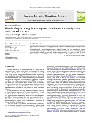
Experimentation with the dynamic policy is performed with the
degree of repair determined by the function a(t)=0.991+0.0093t-
0.03t2
selected idealistically as an example that displays the de-
sired convexity characteristics. This hypothetical function is se-
lected so that the degree of repair is almost perfect (i.e.,
a(0)=0.991) at the beginning of the warranty period and reason-
ably good (i.e., a(3) = 0.75) at the end. In practice, manufacturers
would have a chance to construct a function close to this form by
considering a sequence of progressively decreasing degrees of re-
pair. Fig. 1 shows the percentage difference in the expected cost
relative to the optimum static policy (Eqs. (4) vs. (1)) as a function
of the degree of repair for a Weibull lifetime. It is observed that the
dynamic policy outperforms the optimum static policy when it is
different from perfect repair. That is, the relative performance of
the dynamic policy improves as the fixed component of the cost
function decreases and the mean time to the first failure increases.
On the other hand, for products with a normal failure distribution,
Fig. 2 shows that for smaller ratios of the fixed to variable cost
component, the dynamic policy performs better only when the
product quality is either low or high. When the fixed cost compo-
nent is much larger than the variable component, the dynamic pol-
icy always dominates the optimum static repair policy. The
difference in the trends seen in Figs. 1 and 2 may be attributable
to the greater sensitivity of the expected number of failures to
the degree of repair under a Weibull distribution.
5.2.2. Results with two-dimensional warranties
Along the same lines in Section 5.2.1, we set the shape param-
eters of both the time and usage dimensions at 2, and manipulate
the two scale parameters to vary the mean time and usage until the
first failure. Table 7 shows the effects of product reliability and the
degree of repair on the expected number of breakdowns (Eq. (9))
with various static policies both under Weibull and Normal life-
Table 4
Optimum static repair degree for various first interarrival mean and cost ratios under
a Weibull lifetime
Table 5
Optimum static repair degree for various first interarrival mean and cost ratios under
a Normal lifetime
Table 6
Difference in expected cost between optimal static and improved repair policies
b l1 c/c1 = 0 (%) c/c1 = 5 (%) c/c1 = 10 (%) c/c1 = 100 (%)
Weibull lifetime
0.56 0.50 28.39 31.17 31.42 31.69
1.16 1.03 10.13 16.52 17.10 17.72
1.76 1.56 À2.71 9.09 10.00 10.98
2.36 2.09 À19.28 4.63 5.76 6.98
2.96 2.62 À36.65 2.02 3.29 4.64
3.56 3.15 À54.50 0.47 1.81 3.24
4.16 3.69 À72.58 À0.51 0.88 2.36
4.76 4.22 À86.60 À1.35 0.26 1.77
5.36 4.75 À97.19 À2.22 À0.17 1.36
5.66 5.01 À107.19 À5.89 À3.55 À2.01
l1 c/c1 = 0 (%) c/c1 = 1 (%) c/c1 = 10 (%) c/c1 = 100 (%) c/c1 = 1000 (%)
Normal lifetime
0.5 37.06 38.25 39.23 39.42 39.44
1.4 1.00 8.23 13.09 14.05 14.16
2.0 À40.77 À7.05 2.32 3.82 3.99
3.2 À126.27 À38.29 À3.22 À0.02 0.15
4.1 À134.92 À43.57 À4.69 À0.18 0.04
5.0 À137.42 À45.09 À5.53 À0.29 0.01
-10
0
10
20
30
40
50
60
70
80
90
100
0.00 1.00 2.00 3.00 4.00 5.00 6.00
Mean time to the first failure
Differenceinexpectedcost(%)
c/c1=0 c/c1=1 c/c1=10 c/c1=1000
Fig. 1. Expected cost under dynamic policy relative to the optimum static policy
under a Weibull lifetime.
-60
-40
-20
0
20
40
60
80
0 1 2 3 4 5 6
Mean time to the first failure
Differenceinexpectedcost(%)
c/c1=0 c/c1=1 c/c1=10
Fig. 2. Expected cost under dynamic policy relative to the optimum static policy
under a Normal lifetime.
638 G. Samatlı-Paç, M.R. Taner / European Journal of Operational Research 197 (2009) 632–641

8. times. Results indicate that for a given mean vector (l1,l2), the ex-
pected number of failures increases as the degree of repair de-
creases along at least one-dimension. In parallel with the results
under one-dimensional warranties, when the product reliability
deteriorates, the expected number of failures increases
significantly.
Table 8 investigates the effect of the correlation coefficient (q)
varied as 0.2, 0.5 and 0.9 under various static policies. It is observed
that as the time and usage dimensions become more dependent on
each other, the expected number of failures (Eq. (9)) increases. Re-
sults suggest no significant interaction between the degree of re-
pair (a1,a2) and the correlation coefficient.
Table 7
Expected number of failures under various static policies (q = 0.2)
(a1,a2) l1 = l2 l1 – l2
(5,5) (3,3) (1.5,1.5) (5,3) (5,1) (3,1)
Weibull lifetime
(1.0,1.0) 0.090153 0.338829 1.15429 0.163960 0.257874 0.620392
(1.0,0.8) 0.090466 0.343277 1.22612 0.164710 0.258058 0.62301
(1.0,0.5) 0.091333 0.354343 1.34137 0.166356 0.258111 0.82
(0.8,1.0) 0.090466 0.343277 1.22612 0.165217 0.264394 0.659544
(0.8,0.8) 0.090917 0.349766 1.34158 0.166384 0.264819 0.666086
(0.8,0.5) 0.092233 0.367364 1.35 0.168995 0.265148 0.82
(0.5,1.0) 0.091333 0.354343 1.34137 0.169103 0.292529 0.817921
(0.5,0.8) 0.092233 0.367364 1.35 0.17247 0.295131 0.82
(0.5,0.5) 0.095038 0.416865 1.35 0.180836 0.296013 0.82
Normal lifetime
(1.0,1.0) 0.006120 0.282020 1.30157 0.035645 0.054791 0.502419
(1.0,0.8) 0.006120 0.282058 1.42095 0.036123 0.054793 0.504250
(1.0,0.5) 0.006120 0.282265 1.52067 0.036126 0.054810 0.504940
(0.8,1.0) 0.006120 0.282058 1.42095 0.036123 0.054840 0.506542
(0.8,0.8) 0.006120 0.282148 1.61625 0.036125 0.054847 0.506548
(0.8,0.5) 0.006120 0.282678 1.83357 0.036134 0.054849 0.506591
(0.5,1.0) 0.006120 0.282265 1.52067 0.036130 0.055404 0.541821
(0.5,0.8) 0.006120 0.282678 1.83357 0.036142 0.055510 0.543897
(0.5,0.5) 0.006123 0.285225 1.84 0.036208 0.055614 0.545218
Table 8
Expected number of failures under various static policies with equal means and different correlation values
(a1,a2) q l1 = l2 l1 = l2
(5,5) (3,3) (1.6,1.6) (5,5) (3,3) (1.5,1.5)
Weibull lifetime Normal lifetime
(1.0,1.0) 0.2 0.090153 0.338829 1.154290 0.006120 0.282020 1.30157
0.5 0.138094 0.409353 1.243220 0.013815 0.333447 1.35608
0.9 0.222465 0.565944 1.565110 0.035227 0.429388 1.46380
(0.8,0.8) 0.2 0.090917 0.349766 1.341580 0.006120 0.282148 1.61625
0.5 0.140160 0.428501 1.469650 0.013816 0.333965 1.67354
0.9 0.228486 0.608947 1.830538 0.035243 0.431593 1.81255
(0.5,0.5) 0.2 0.095038 0.416865 1.84 0.006123 0.285225 1.82
0.5 0.151606 0.503631 1.84 0.013841 0.341547 1.82
0.9 0.25765 0.696287 1.84 0.035471 0.454591 1.82
Table 9
Optimal degree combination for static repair (c = c1,q = 0.2)
c¼c1
c2
l1 = l2 l1 – l2
(5,5) (3,3) (1.5,1.5) (5,3) (5,1) (3,1) (2,1.6)
Weibull lifetime
0.1 (0.5,0.5) (0.5,0.5) (1.0,0.5) (0.8,0.5) (0.8,0.5) (1.0,0.8) (1.0,0.8)
1 (0.5,0.5) (0.5,0.5) (1.0,0.5) (0.5,0.5) (0.5,0.5) (0.8,0.8) (1.0,0.8)
10 (0.5,0.8) (0.5,1.0) (0.5,1.0) (0.5,1.0) (0.5,0.5) (0.8,0.8) (0.5,1.0)
10000 (0.5,1.0) (0.5,1.0) (0.5,1.0) (0.5,1.0) (0.5,1.0) (0.8,1.0) (0.5,1.0)
c¼c1
c2
l1 = l2 l1 – l2
(5,5) (3,3) (1.5,1.5) (5,3) (5,1) (3,1) (2,1.5)
Normal lifetime
0.1 (0.5,0.5) (0.5,0.5) (1.0,0.5) (0.5,0.5) (0.5,0.5) (0.5,0.5) (1.0,0.5)
1 (0.5,0.5) (0.5,0.5) (1.0,0.5) (0.5,0.5) (0.5,0.5) (0.5,0.5) (1.0,0.5)
10 (0.5,0.5) (0.5,0.5) (0.5,1.0) (0.5,0.5) (0.5,0.5) (0.5,0.5) (0.5,1.0)
10000 (0.5,1.0) (0.5,1.0) (0.5,1.0) (0.5,1.0) (0.5,1.0) (0.5,1.0) (0.5,1.0)
G. Samatlı-Paç, M.R. Taner / European Journal of Operational Research 197 (2009) 632–641 639

9. Samatlı (2006) observes that when the variable components of
the cost function are equal to each other, the ratio of the fixed com-
ponent to the variable components affects the selection of the opti-
mal repair policy in a similar way as in one-dimensional warranty.
Table 9 presents the optimal degree of static repair for different
relative magnitudes of the two variable components. The fixed cost
component is set equal to one of the variable components as c = c1.
Results indicate that the optimum degree of repair tends to be lar-
ger for the dimension with a lower variable cost component.
As in one-dimensional warranty, the improved policy for a reli-
able product offers no advantages over a perfect repair in terms of
the expected number of failures. Table 10 analyzes the perfor-
mance of the improved policy relative to the optimum static policy
in terms of the expected cost (Eqs. (1) vs. (3)). When the fixed com-
ponent of the cost function is significantly larger than the variable
components, the improved policy generally dominates the opti-
mum static policy, which turns out to be perfect repair.
For the two-dimensional dynamic policy, the degree of repair
for the time dimension is determined by the same function as in
the one-dimensional case and the degree of repair for the usage
dimension is calculated such that a2;i ¼ a1ð
PiÀ1
k¼1TkÞ l2
l1
. Table 11
shows the percentage difference between the dynamic and optimal
static policies (Eqs. (1) vs. (5)) where a negative sign indicates that
the cost of optimal static policy is smaller than that of dynamic.
The relative performance of the dynamic policy improves under a
Weibull lifetime when the fixed component of the cost decreases.
Performance of the dynamic policy under a Normal lifetime dis-
plays an analogous behavior to that observed in Fig. 2 in the sin-
gle-dimensional analysis.
6. Conclusion
Computational results show that the dynamic policy generally
outperforms both static and improved policies on highly reliable
products, whereas the improved policy is the best performer for
products with low reliability. Although, the increasing number of
factors arising in the analysis of two-dimensional policies renders
generalizations difficult, several insights are offered for the selec-
tion of the rectification action based on empirical evidence.
As a future direction, the analysis can be extended to multi-
dimensional warranties. For example, a three-dimensional quasi-
renewal process may be used to model the warranty policy offered
for the flight engines. In addition, the study can be generalized to
accommodate multi-component systems. In this case, each compo-
nent failure process may be modeled as a quasi-renewal process.
Acknowledgement
The authors would like to thank the two anonymous referees
for their helpful suggestions and constructive comments on an ear-
lier version of this manuscript.
References
Bai, J., Pham, H., 2005. Repair-limit risk-free warranty policies with imperfect
repair. IEEE Transactions on Systems, Man and Cybernetics, Part A 35 (6),
765–772.
Barlow, R., Hunter, L., 1960. Optimum preventive maintenance policies. Operations
Research 8, 90–100.
Boland, P.J., Proschan, F., 1982. Periodic replacement with increasing minimal repair
costs at failure. Operations Research 30 (6), 1183–1189.
Choi, C.H., Yun, W.Y., 2006. A repair cost limit policies with fixed warranty
period. In: Yun, W.Y., Dohi, T. (Eds.), Advanced reliability modeling II:
reliability testing and improvement: Proceedings of the Second International
Workshop Aiwarm 2006. World Scientific Publishing Co. Pte. Ltd., Singapore,
2006, pp. 353–360.
Chukova, S., Johnston, M.R., 2006. Two-dimensional warranty repair strategy based
on minimal and complete repairs. Mathematical and Computer Modeling 44,
1133–1143.
Chukova, S., Hayakawa, Y., Johnston, M.R., 2006. Two-dimensional warranty:
Minimal/complete repair strategy. In: Yun, W.Y., Dohi, T. (Eds.), Advanced
reliability modeling II: Reliability testing and improvement: Proceedings of the
Second International Workshop Aiwarm 2006. World Scientific Publishing Co.
Pte. Ltd., Singapore, 2006, pp. 361–368.
Cleroux, R., Dubuc, S., Tilquin, C., 1979. The age replacement with minimal repair
and random repair costs. Operations Research 27 (6), 1158–1167.
Cohen, A.C., Whitten, B.J., 1988. Parameter Estimation in Reliability and Life Span
Models. Marcel Dekker Inc., New York and Basel.
Dagpunar, J.S., 1997. Renewal-type equations for a general repair process. Quality
and Reliability Engineering International 13, 235–245.
Table 10
Percentage difference in the expected cost under optimal static and improved repair
policies (c1 = c2)
c
c1¼c2
q l1 = l2 l1 – l2
(5,5) (3,3) (1.6,1.6) (5,3) (5,1) (3,1)
Weibull lifetime
1 0.2 À60.47 À35.65 À5.57 À52.82 À45.33 À15.81
0.5 À53.30 À34.12 À7.28 À47.01 À46.02 À15.96
0.9 À34.52 À26.69 À2.83 À45.47 À45.06 À15.75
10 0.2 À6.80 À2.04 5.39 À5.66 À6.13 À0.27
0.5 À5.12 À0.61 5.99 À5.39 À6.70 À0.74
0.9 À3.29 1.50 8.04 À5.95 À6.19 À1.07
10000 0.2 0.40 1.53 7.92 1.16 1.56 3.90
0.5 0.79 2.35 8.37 1.56 1.37 3.80
0.9 1.48 3.75 10.39 1.41 1.48 3.98
c
c1¼c2
q l1 = l2 l1 – l2
(5,5) (3,3) (1.5,1.5) (5,3) (5,1) (3,1)
Normal lifetime
1 0.2 À55.23 À58.18 À0.79 À60.63 À66.07 À55.23
0.5 À57.62 À57.64 À4.21 À63.70 À66.19 À55.47
0.9 À59.35 À54.12 À11.84 À66.11 À66.46 À55.35
10 0.2 À2.93 À4.89 10.52 À6.99 À11.09 À8.31
0.5 À4.52 À4.53 10.72 À9.25 À11.17 À8.31
0.9 À5.66 À4.17 10.97 À11.11 À11.32 À8.24
10000 0.2 8.64 5.89 13.41 3.43 0.01 0.26
0.5 7.10 5.01 13.60 2.24 À0.02 0.26
0.9 5.61 4.02 13.84 0.02 À0.02 0.26
Table 11
Percentage difference in the expected cost under optimal static and dynamic repair
policies (c1 = c2)
c
c1¼c2
q l1 = l2 l1 – l2
(5,5) (3,3) (1.6,1.6) (5,3) (5,1) (3,1)
Weibull lifetime
1 0.2 45.49 9.07 8.08 49.87 53.71 36.47
0.5 47.53 11.80 6.51 51.55 53.53 36.54
0.9 50.37 12.74 8.94 52.14 53.99 36.41
10 0.2 14.45 7.91 5.44 15.92 15.57 11.86
0.5 15.07 8.44 5.78 15.69 15.19 11.57
0.9 14.33 6.46 6.34 15.32 15.88 10.66
10000 0.2 2.90 2.87 3.59 3.49 3.96 3.67
0.5 2.45 2.71 3.76 3.43 4.01 3.69
0.9 2.37 2.70 4.43 3.80 4.37 3.16
c
c1¼c2
q l1 = l2 l1 – l2
(5,5) (3,3) (1.5,1.5) (5,3) (5,1) (3,1)
Normal lifetime
1 0.2 31.07 À15.48 À1.60 36.38 41.68 14.36
0.5 30.10 À15.10 À1.24 36.56 41.60 14.20
0.9 29.42 À12.56 À7.75 37.24 43.77 15.07
10 0.2 11.97 2.87 À1.02 13.80 15.73 13.25
0.5 10.78 3.15 À0.57 14.03 15.61 11.71
0.9 9.96 3.34 À0.07 14.93 19.66 14.68
10000 0.2 7.69 5.89 À2.76 7.35 8.98 6.00
0.5 6.32 4.96 À2.38 8.46 8.90 5.95
0.9 5.00 3.78 À1.88 9.00 10.93 7.67
640 G. Samatlı-Paç, M.R. Taner / European Journal of Operational Research 197 (2009) 632–641

10. Davis, D.J., 1952. An analysis of some failure data. Journal of the American Statistical
Association 47, 113–150.
Dimitrov, B., Chukova, S., Khalil, Z., 2004. Warranty costs: An age-dependent failure/
repair model. Naval Research Logistics 51 (7), 959–976.
Iskandar, B.P., Murthy, D.N.P., 2003. Repair–replace strategies for two-dimensional
warranty policies. Mathematical and Computing Modeling 38, 1233–1241.
Iskandar, B.P., Murthy, D.N.P., Jack, N., 2005. A new repair–replace strategy for items
sold with a two-dimensional warranty. Computers and Operations Research 32,
669–682.
Karim, M.R., Suzuki, K., 2005. Analysis of warranty claim data: A literature
review. International Journal of Quality and Reliability Management 22 (7),
667–686.
Kijima, M., 1989. Some results for repairable systems with general repair. Journal of
Applied Probability 26, 89–102.
Murthy, D.N.P., Blischke, W.R., 1992a. Product warranty management – II: An
integrated framework for study. European Journal of Operational Research 62,
261–281.
Murthy, D.N.P., Blischke, W.R., 1992b. Product warranty management – III: A review
of mathematical models. European Journal of Operational Research 63, 1–34.
Murthy, D.N.P., Djamaludin, I., 2002. New product warranty: A literature review.
International Journal of Production Economics 79, 231–260.
Nguyen, D.G., Murthy, D.N.P., 1984. A combined block and repair limit replacement
policy. Journal of the Operational Research Society 35 (7), 653–658.
Phelps, R.I., 1983. Optimal policy for minimal repair. Journal of the Operational
Research Society 34 (5), 425–427.
Samatlı, G., 2006. Warranty Cost Analysis Under Imperfect Repair. Unpublished
Masters Thesis, Bilkent University, Ankara, Turkey.
Thomas, M.U., Rao, S.S., 1999. Warranty economic decision models: A summary and
some suggested directions for future research. Operations Research 47 (6), 807–
820.
Wang, H., Pham, H., 1996a. Optimal maintenance policies for several imperfect
repair models. International Journal of Systems Science 27 (6), 543–549.
Wang, H., Pham, H., 1996b. A quasi renewal process and its applications in
imperfect maintenance. International Journal of Systems Science 27 (10), 1055–
1062.
Yanez, M., Joglar, F., Modarres, M., 2002. Generalized renewal process for analysis of
repairable systems with limited failure experience. Reliability Engineering and
System Safety 77, 167–180.
G. Samatlı-Paç, M.R. Taner / European Journal of Operational Research 197 (2009) 632–641 641