This paper analyzes optimal reinstatement strategies for short-tail excess of loss reinsurance programs, highlighting that mirror layers and certain reinstatement premium protections are often sub-optimal. It examines the impact of reinstatement alternatives, the calculation of break-even reinsurance premiums, and compares various strategies based on their effectiveness and costs. The findings aim to provide a clearer understanding of how to structure reinsurance in a manner that aligns motivation between insurers and reinsurers.

1. Reinstatement strategy: philosophy, theory, and practice
Richard Hartigan FIA FIAA BEc MBA
Abstract
This paper determines the optimal reinstatement strategy for an insurer’s short-tail
excess of loss reinsurance programme. Mirror layers, 1-shot layers (with or without
back-up layers), and reinstatement premium protection will almost certainly be sub-
optimal.
Keywords: Reinsurance, Reinstatement Premium, Capital
Correspondence to: richard_hartigan@hotmail.com
Special thanks to Paul Johnson for review, comments, and challenge.
2 March 2017
Other papers in the series from the same author:
• Quota share reinsurance: philosophy, theory, and practice (21 August 2015)
• Capital-optimal reinsurance strategy: philosophy, theory, and practice (14 April 2016)

2. Reinstatement strategy: philosophy, theory, and practice (Richard Hartigan)
2 2 March 2017
Survey of prior research
Anderson & Dong (1988) incorporated reinstatement premiums as a standard feature of
excess of loss catastrophe reinsurance, but were principally concerned with the (then
relatively new) use of catastrophe models to price catastrophe risk.
Mata (2000) focussed on how splitting longer layers in an excess of loss reinsurance
programme into smaller sub-layers affected the theoretical price of the longer layer versus
the theoretical price of the sum of the smaller sub-layers, under varying reinstatement
premium provisions.
Campana (2011) focussed on the initial risk adjusted premium by varying the number of
reinstatements, with the reinstatement premium provision fixed at 100%.
Introduction
Short-tail excess of loss reinsurance programmes are typically placed in a tower of
ascending layers, above the insurer’s net retention. For example, the insurer may choose to
retain the first $4m of each loss (this becomes the insurer’s net retention) and buy $46m of
excess of loss reinsurance above the net retention as follows: $6m excess of $4m (i.e. $6m
x $4m), plus $10m excess of $10m (i.e. $10m x $10m), plus $30m excess of $20m (i.e.
$30m x $20m).
The reinsurance premium for a layer is often expressed as a Rate-On-Line (ROL), and this is
simply the reinsurance premium for the layer (e.g. $3.3m) divided by the size of the layer
(e.g. $30m for the $30m x $20m layer). The ROL in that instance is $3.3m / $30m = 11%.
Typically, cover is not unlimited for multiple events in a given time period (which is typically 1
year). The most-typical cover limitation (i.e. reinstatement alternative) is expressed as
1@100%, which means the layer must be reinstated once (after the first loss) with the
payment of an additional reinsurance premium (i.e. the reinstatement premium) of 100% of
the original reinsurance premium (and note: not pro-rata for the remaining time period of
cover). The reinstatement typically happens automatically and without optionality (for either
party).
An example will clarify: the ROL for the $6m x $4m layer is 25% (i.e. a reinsurance premium
of $1.5m), and cover incepts on 1 January 2016. A $10m qualifying event occurs on 15
February 2016. The insurer recovers $6m (after retaining the first $4m of the loss) from the
reinsurer, and then reinstates the layer by paying a reinstatement premium of $1.5m. In
practice, the $1.5m is simply netted off the $6m when the reinsurer pays the insurer. A
second $10m qualifying event occurs on 25 July 2016. Again, the insurer recovers $6m
(after retaining the first $4m of the loss) from the reinsurer. Having recovered a second time
the layer is now exhausted and no further reinstatements are permitted. For the $6m x $4m
layer for the balance of the year (i.e. 25 July 2016 to 31 December 2016) the insurer has no
cover for losses.
Reinstatement alternatives vary. 1@100% is by far the most common but 1@200% and
1@300% are also observed, especially when the ROL is low. Straight multiples of 100% are
not mandatory; for example 1@125% is occasionally observed. More than one
reinstatement is possible; for example 2@100%.
Other reinstatement alternatives exist. 1@free is self-explanatory. Cover might be 1-shot,
i.e. with zero reinstatements. Cover might be back-up, i.e. covering the second loss only.
As an aside (and I shall prove this later) the theoretical reinsurance premium for a 1@free

3. Reinstatement strategy: philosophy, theory, and practice (Richard Hartigan)
3 2 March 2017
layer is identical to the sum of the theoretical reinsurance premium for a 1-shot layer plus the
theoretical reinsurance premium for a back-up layer.
Other reinstatement alternatives exist. The insurer can buy a 1@100% layer, and then
separately buy reinstatement premium protection (RPP) to cover the reinstatement premium.
As an aside (and I shall prove this later) the theoretical reinsurance premium for a 1@free
layer is identical to the sum of the theoretical reinsurance premium for a 1@100% layer plus
the theoretical reinsurance premium for RPP. Another reinstatement alternative is a so-
called mirror layer: the insurer overbuys a given layer so that any recovery additionally funds
the reinstatement premium due.
Probability of loss
I start with the assumption that, for a given layer, the probability of attaching (i.e. a qualifying
event being equal to the bottom of the layer) equals the probability of exhaustion (i.e. a
qualifying event being equal to the top of the layer). This assumption is valid if the size of
the layer is relatively small, say $1 reductio ad absurdum.
Having made the above assumption I model using a Poisson probability distribution. I note
that other discrete probability distributions (e.g. Negative Binomial) may be more appropriate
for certain perils, certain geographical regions, and/or certain layers in an excess of loss
reinsurance programme.
Poisson: P(k events in 1 year) = λ^k.e^(-λ) / k!
Assume the probability of 1 or more events in 1 year is X. Therefore λ = -LN(100%-X) and:
P0 = e^(-λ)
P1 = e^(-λ).λ
P2+ = 1 - P0 - P1 (for the balance of this paper I shall use P2 to denote P2+)
Quantum of the net loss
Focussing (for the moment) on just the 1@100% reinstatement alternative, there are three
outcomes.
0 losses in which case the reinsurance premium (ROLgross) is paid
1 loss in which case the reinsurance premium (ROLgross) is paid, one recovery is made,
the reinstatement premium is paid
2+ losses in which case the reinsurance premium (ROLgross) is paid, one recovery is made,
the reinstatement premium is paid, a second recovery is made
At this stage I must recognise an additional factor. Typically, excess of loss reinsurance
programmes are placed by a broker who receives brokerage (B, typically 10% of the
reinsurance premium). Thus the reinsurer receives less than 100% of the reinsurance
premium. Further complicating this issue is that brokerage is typically only payable on the
original reinsurance premium, not on any additional reinsurance premium (i.e. the
reinstatement premium). Complicating matters further is the fact that often the broker
rebates part of the brokerage received back to their client (the insurer) (R, typically 25% of
the brokerage).

4. Reinstatement strategy: philosophy, theory, and practice (Richard Hartigan)
4 2 March 2017
The reinsurer will calculate the burn (break-even) reinsurance premium (ROLburn) as follows:
0 = P0 * ((1 - B) * ROLburn - 0)
+ P1 * ((2 - B) * ROLburn - 1)
+ P2 * ((2 - B) * ROLburn - 2)
Solving: ROLburn = (1 - P0 + P2) / (2 - 1 * P0 - B)
Using a similar approach for other reinstatement alternatives:
1@free: ROLburn = (1 - P0 + P2) / (1 - 0 * P0 - B)
1@100%: ROLburn = (1 - P0 + P2) / (2 - 1 * P0 - B)
1@200%: ROLburn = (1 - P0 + P2) / (3 - 2 * P0 - B)
1@300%: ROLburn = (1 - P0 + P2) / (4 - 3 * P0 - B)
1-shot: ROLburn = (1 - P0) / (1 - B)
back-up: ROLburn = P2 / (1 - B)
Determining the burn (break-even) reinsurance premium (ROLburn)
From above the ROLburn (1@100%) = (1 - P0 + P2) / (2 - 1 * P0 - B), and B = 10%.
Assume the probability of 1 or more events in 1 year is 20% (i.e. X).
Therefore λ = 22.31% (i.e. -LN(100%-X)).
Therefore:
P0 = 80.00% (i.e. e^(-λ), from above)
P1 = 17.85% (i.e. e^(-λ).λ, from above)
P2 = 2.15% (i.e. 1 - P0 - P1, from above)
Therefore the burn (break-even) reinsurance premium, ROLburn (1@100%) = 20.14%.
What is of more interest though is the equivalent burn (break-even) reinsurance premium
(ROLburn) for different reinstatement alternatives, and at different ROLburn levels. The table
below gives an abbreviated summary (I select ROLburn (1@100%) at whole percentages):
1@300% 1@200% 1@100% 1-shot 1@free back-up mirror RPP
0.98% 0.98% 1.00% 1.00% 1.00% 0.00% 1.01% 0.01%
4.55% 4.76% 5.00% 5.13% 5.25% 0.12% 5.26% 0.26%
8.40% 9.13% 10.00% 10.53% 11.05% 0.52% 11.11% 1.05%
11.73% 13.16% 15.00% 16.18% 17.42% 1.24% 17.65% 2.43%
14.69% 16.94% 20.00% 22.06% 24.41% 2.35% 25.00% 4.41%
17.37% 20.50% 25.00% 28.12% 32.03% 3.90% 33.33% 7.03%
19.85% 23.89% 30.00% 34.33% 40.29% 5.96% 42.86% 10.30%
This table can be interpreted (by example) as follows: the insurer and the reinsurer will be
similarly motivated between engaging in a 1@100% layer at 10.00% ROLburn and engaging
in a 1@300% layer at 8.40% ROLburn. Note: the mirror layer ROLburn = 100% / (100% -
ROLburn (1@100%)), and is the sum of the 1@100% layer and the mirror layer itself.

5. Reinstatement strategy: philosophy, theory, and practice (Richard Hartigan)
5 2 March 2017
As an aside, one can see (subject to minor rounding errors):
1@free = 1-shot + back-up; and
1@free = 1@100% + RPP (where RPP = 1@100% * 1-shot)
= 1@100% (1 + 1-shot)
Proof (formulae on Page 4):
1@free: ROLburn = (1 - P0 + P2) / (1 - 0 * P0 - B) = (1 - P0 + P2) / (1 - B)
1@100%: ROLburn = (1 - P0 + P2) / (2 - 1 * P0 - B) = (1 - P0 + P2) / (2 - P0 - B)
1-shot: ROLburn = (1 - P0) / (1 - B)
back-up: ROLburn = P2 / (1 - B)
1-shot + back-up= (1 - P0) / (1 - B) + P2 / (1 - B) = (1 - P0 + P2) / (1 - B) = 1@free
1@100% + RPP = 1@100% (1 + 1-shot)
= (1 - P0 + P2) / (2 - P0 - B) * [1 + (1 - P0) / (1 - B)]
= (1 - P0 + P2) / (2 - P0 - B) * [(1 - B + 1 - P0) / (1 - B)]
= (1 - P0 + P2) / (2 - P0 - B) * [(2 - P0 - B) / (1 - B)]
= (1 - P0 + P2) / (1 - B)
= 1@free
Determining the gross (loaded) reinsurance premium (ROLgross)
The reinsurer is naturally profit-seeking. The above ROLburn figures need to be loaded.
Each reinsurer will have their own method for doing so, and therefore I must choose a
simple and sensible method. I simply add the square root of the burn (break-even)
reinsurance premium (ROLburn). For example: the square root of 15% is 3.87%, and
therefore the gross (loaded) reinsurance premium (ROLgross) would be 18.87%. This method
results in sensible expected reinsurance recovery rates (expected total reinsurance
recoveries / expected total reinsurance premium), both by reinstatement alternative and by
ROLgross level.
The table below gives an abbreviated summary (I re-select ROLgross (1@100%) at whole
percentages):
1@300% 1@200% 1@100% 1-shot 1@free back-up mirror RPP
0.99% 0.99% 1.00% 1.00% 1.00% 0.03% 1.01% 0.04%
4.74% 4.86% 5.00% 5.06% 5.12% 0.27% 5.26% 0.43%
8.92% 9.42% 10.00% 10.33% 10.64% 0.78% 11.11% 1.30%
12.59% 13.68% 15.00% 15.82% 16.63% 1.55% 17.65% 2.62%
15.86% 17.67% 20.00% 21.51% 23.11% 2.63% 25.00% 4.44%
18.82% 21.44% 25.00% 27.38% 30.11% 4.05% 33.33% 6.78%
21.54% 25.02% 30.00% 33.43% 37.69% 5.88% 42.86% 9.68%
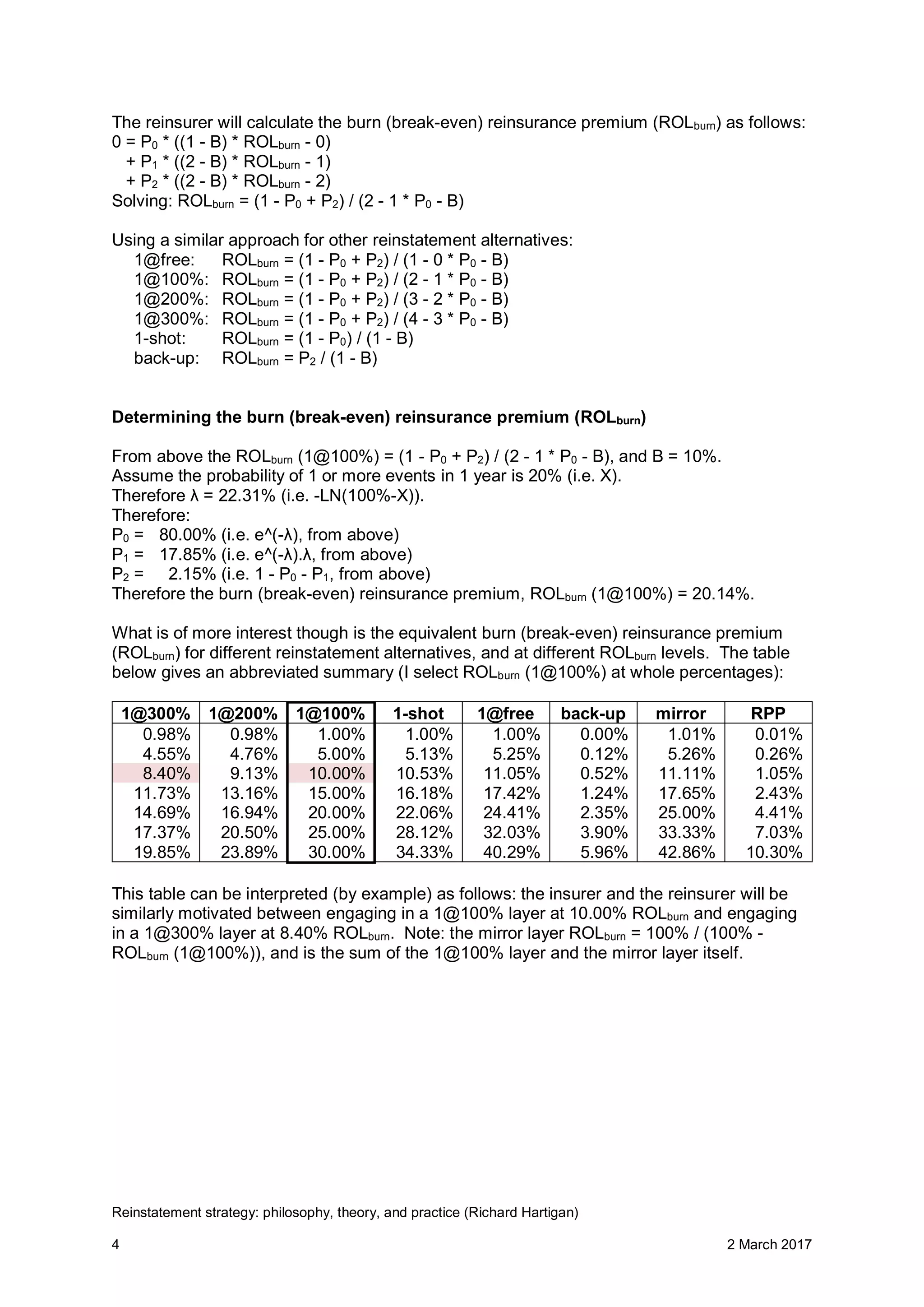
This table can be interpreted (by example) as follows: the insurer and the reinsurer will be
similarly motivated between engaging in a 1@100% layer at 10.00% ROLgross and engaging
in a 1@300% layer at 8.92% ROLgross. Note: the mirror layer ROLgross = 100% / (100% -
ROLgross (1@100%)), and is the sum of the 1@100% layer and the mirror layer itself.

6. Reinstatement strategy: philosophy, theory, and practice (Richard Hartigan)
6 2 March 2017
Comparing reinstatement alternatives
I now compare reinstatement alternatives (as follows), and at different ROLgross levels:
• 1@300%
• 1@200%
• 1@100%
• 1@free
• 1-shot, paired with a back-up
• 1@100%, paired with a mirror layer, such that any recovery additionally funds the
reinstatement premium due for the first loss
• 1@100%, paired with RPP
The latter three reinstatement alternatives can immediately be identified as being
administratively more cumbersome as they involve buying two ‘things’ rather than just one
‘thing’. It turns out that they are also more capital-intensive, and incur more brokerage. In
addition, the mirror layer reinstatement alternative results in an over-recovery for the second
loss (when the reinstatement premium would not be payable).
To assess the optimal reinstatement strategy I must maximise expected profit to the insurer
from reinsuring (as % layer), using (in the case of the 1@100% reinstatement alternative):
P0 * (0 - (1 - B * R) * ROLgross)
+ P1 * (1 - (2 - B * R) * ROLgross)
+ P2 * (2 - (2 - B * R) * ROLgross)
It should be readily apparent that the expected profit to the insurer from reinsuring will be
negative.
Calculations for all reinstatement alternatives, and at different ROLgross levels, are on the
page following.
Expected profit to the insurer from reinsuring (as % layer)
ROLgross
(1@100%)
1@300% 1@200% 1@100% 1@free 1 shot +
back-up
mirror
(1@100%)
RPP
(1@100%)
1.00% -0.6307% -0.6299% -0.6378% -0.6344% -0.6598% -0.6443% -0.6726%
2.00% -1.0627% -1.0593% -1.0639% -1.0525% -1.1158% -1.0857% -1.1529%
3.00% -1.4308% -1.4238% -1.4193% -1.4096% -1.5169% -1.4632% -1.5674%
4.00% -1.7615% -1.7499% -1.7440% -1.7269% -1.8803% -1.8166% -1.9526%
5.00% -2.0697% -2.0530% -2.0482% -2.0200% -2.2210% -2.1559% -2.3179%
6.00% -2.3650% -2.3426% -2.3320% -2.2986% -2.5487% -2.4809% -2.6638%
7.00% -2.6526% -2.6238% -2.5957% -2.5682% -2.8690% -2.7911% -2.9910%
8.00% -2.9288% -2.8933% -2.8589% -2.8257% -3.1774% -3.1075% -3.3166%
9.00% -3.1965% -3.1540% -3.1216% -3.0741% -3.4770% -3.4303% -3.6407%
10.00% -3.4610% -3.4111% -3.3740% -3.3186% -3.7736% -3.7488% -3.9552%
11.00% -3.7236% -3.6657% -3.6161% -3.5604% -4.0684% -4.0631% -4.2605%
12.00% -3.9820% -3.9160% -3.8577% -3.7977% -4.3591% -4.3838% -4.5647%
13.00% -4.2374% -4.1627% -4.0988% -4.0316% -4.6465% -4.7112% -4.8678%
14.00% -4.4904% -4.4067% -4.3392% -4.2628% -4.9317% -5.0455% -5.1700%
15.00% -4.7445% -4.6513% -4.5692% -4.4946% -5.2183% -5.3755% -5.4634%
16.00% -4.9945% -4.8914% -4.8080% -4.7222% -5.5005% -5.7239% -5.7637%
17.00% -5.2465% -5.1331% -5.0364% -4.9512% -5.7850% -6.0679% -6.0554%
18.00% -5.4952% -5.3712% -5.2734% -5.1770% -6.0661% -6.4310% -6.3537%
19.00% -5.7466% -5.6114% -5.4997% -5.4049% -6.3503% -6.7898% -6.6436%
20.00% -5.9981% -5.8513% -5.7248% -5.6328% -6.6347% -7.1560% -6.9327%
21.00% -6.2474% -6.0886% -5.9582% -5.8583% -6.9166% -7.5420% -7.2280%
22.00% -6.4973% -6.3261% -6.1901% -6.0844% -7.1993% -7.9361% -7.5223%
23.00% -6.7482% -6.5640% -6.4204% -6.3110% -7.4831% -8.3382% -7.8155%
24.00% -7.0002% -6.8026% -6.6489% -6.5386% -7.7681% -8.7485% -8.1074%
25.00% -7.2534% -7.0419% -6.8753% -6.7672% -8.0545% -9.1671% -8.3982%

7. Reinstatement strategy: philosophy, theory, and practice (Richard Hartigan)
7 2 March 2017
ROLgross
(1@100%)
1@300% 1@200% 1@100% 1@free 1 shot +
back-up
mirror
(1@100%)
RPP
(1@100%)
26.00% -7.5080% -7.2822% -7.0996% -6.9970% -8.3425% -9.5940% -8.6877%
27.00% -7.7617% -7.5211% -7.3312% -7.2258% -8.6293% -10.0428% -8.9828%
28.00% -8.0171% -7.7612% -7.5602% -7.4561% -8.9180% -10.5003% -9.2763%
29.00% -8.2744% -8.0028% -7.7864% -7.6882% -9.2088% -10.9667% -9.5682%
30.00% -8.5311% -8.2433% -8.0193% -7.9197% -9.4989% -11.4562% -9.8653%
Note: the ROLgross used is the ROLgross (1@100%) equivalent. The green shading indicates
the optimal strategy.
Summary
It is clear that amongst the first four reinstatement alternatives there is little to choose. It
turns out the best reinstatement strategy is as follows:
• if the ROLgross (1@100%) quoted is <1.25% ... ask for a 1@200% quote instead, and
take that;
• if the ROLgross (1@100%) quoted is >1.25% ... ask for a 1@free quote instead, and
take that;
• mirror layers, 1-shot layers (with or without back-up layers), and reinstatement
premium protection will almost certainly be sub-optimal.

8. Reinstatement strategy: philosophy, theory, and practice (Richard Hartigan)
8 2 March 2017
Varying capital assumptions (away from the ‘square root’ method)
• abandoning the ‘square root’ method and instead marking-up ROLburn to ROLgross by a
variable proportion (higher mark-up for lower ROLburn) makes little difference
• retaining the ‘square root’ method and setting the brokerage rebate (R) to 0% makes
little difference
• retaining the ‘square root’ method and setting the brokerage (B) to 0% makes little
difference
Conclusion
Under most reasonable conditions and assumptions, and across the vast majority of the
ROLgross curve (i.e. the excess of loss reinsurance programme), the optimal reinstatement
alternative for the insurer is the 1@free reinstatement alternative.
Naturally the up-front ROLgross will be higher for the 1@free reinstatement alternative,
although not materially so; a selection of ROLgross for comparison purposes is as follows:
1@100% 1@free
1.00% 1.00%
5.00% 5.12%
10.00% 10.64%
15.00% 16.63%
20.00% 23.11%
25.00% 30.11%
30.00% 37.69%
A higher up-front ROLgross might be especially appealing to the reinsurer in the current
challenging market environment. Otherwise the reinsurer should be indifferent. The broker
might be similarly attracted due to brokerage being applied to a higher up-front ROLgross
(remembering that brokerage is typically only payable on the original reinsurance premium,
not on any additional reinsurance premium (i.e. the reinstatement premium)).
The insurer will recognise that they can, on a probability-weighted basis, reduce reinsurance
premiums by opting for the 1@free reinstatement alternative. There will also be
administration benefits, and simpler post-event communication to senior management of the
final net loss from an event.

9. Reinstatement strategy: philosophy, theory, and practice (Richard Hartigan)
9 2 March 2017
Bibliography
Anderson, Richard R. and Dong, Wemin: Pricing catastrophe reinsurance with reinstatement
provisions using a catastrophe model. Casualty Actuarial Society Forum, pages 303–322,
1988.
Campana, Antonella: Risk adjusted premiums for excess of loss reinsurance with
reinstatements. Dipartimento di Scienze Economiche, Gestionali e Sociali
Universita degli Studi del Molise. Mathematical Methods in Economics and Finance – m2
ef,
Vol. 5/6, No. 1, 2010/11.
Mata, Ana J.: Pricing excess of loss reinsurance with reinstatements. Department of
Actuarial Mathematics and Statistics, Heriot-Watt University. ASTIN BULLETIN, Vol. 30, No.
2, 2000, pp. 349-368.