History of theArtificial Neural
Networks
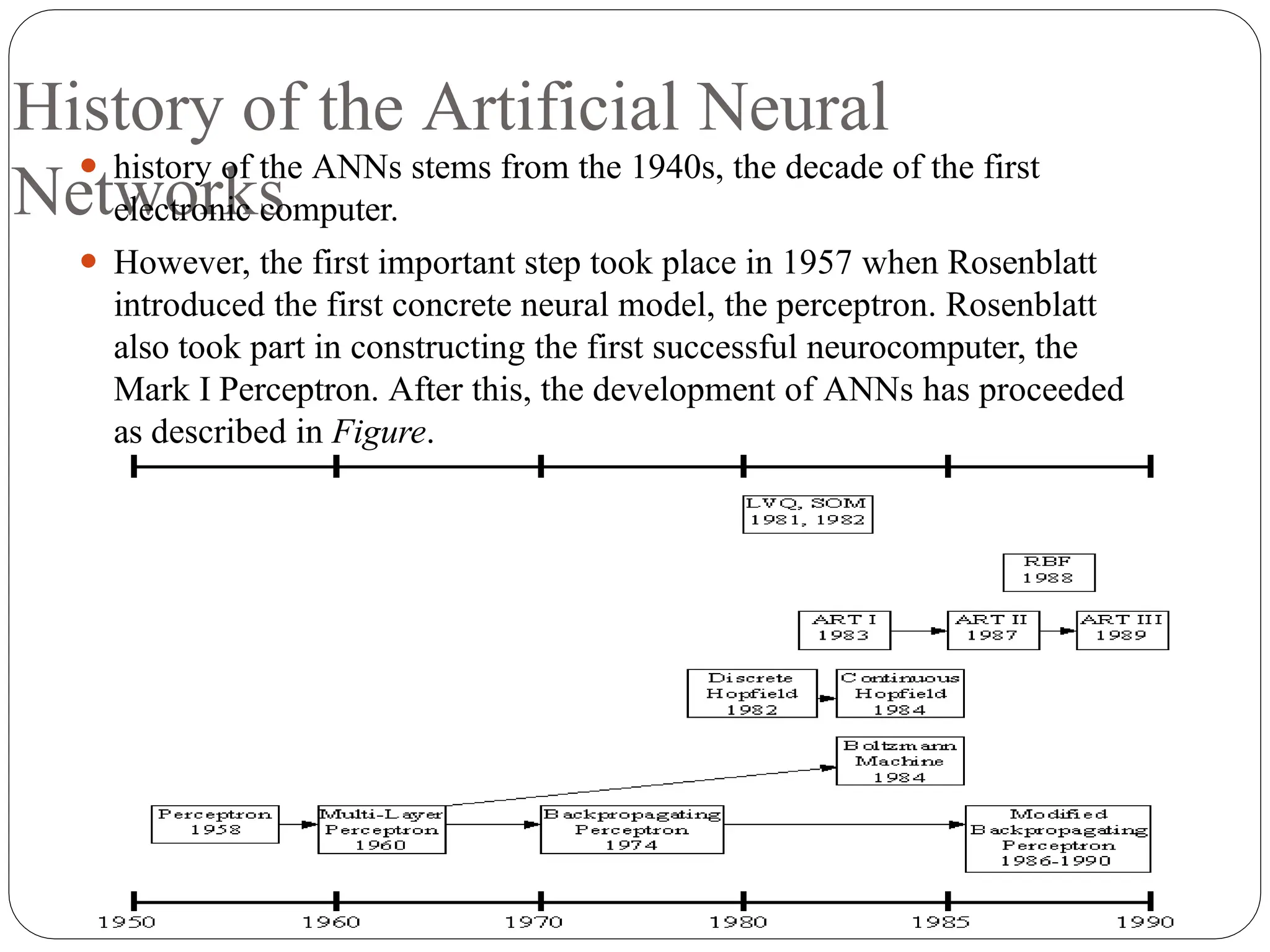
⚫ history of the ANNs stems from the 1940s, the decade of the first
electronic computer.
⚫ However, the first important step took place in 1957 when Rosenblatt
introduced the first concrete neural model, the perceptron. Rosenblatt
also took part in constructing the first successful neurocomputer, the
Mark I Perceptron. After this, the development of ANNs has proceeded
as described in Figure.
2.
History of theArtificial Neural
Networks
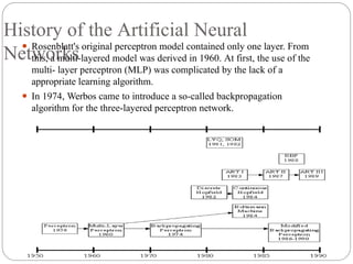
⚫ Rosenblatt's original perceptron model contained only one layer. From
this, a multi-layered model was derived in 1960. At first, the use of the
multi- layer perceptron (MLP) was complicated by the lack of a
appropriate learning algorithm.
⚫ In 1974, Werbos came to introduce a so-called backpropagation
algorithm for the three-layered perceptron network.
3.
History of theArtificial Neural
Networks
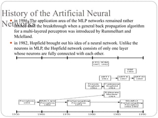
⚫ in 1986, The application area of the MLP networks remained rather
limited until the breakthrough when a general back propagation algorithm
for a multi-layered perceptron was introduced by Rummelhart and
Mclelland.
⚫ in 1982, Hopfield brought out his idea of a neural network. Unlike the
neurons in MLP, the Hopfield network consists of only one layer
whose neurons are fully connected with each other.
4.
History of theArtificial Neural
Networks
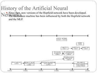
⚫ Since then, new versions of the Hopfield network have been developed.
The Boltzmann machine has been influenced by both the Hopfield network
and the MLP.
5.
History of theArtificial Neural
Networks
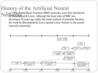
⚫ in 1988, Radial Basis Function (RBF) networks were first introduced
by Broomhead & Lowe. Although the basic idea of RBF was
developed 30 years ago under the name method of potential function,
the work by Broomhead & Lowe opened a new frontier in the neural
network community.
6.
History of theArtificial Neural
Networks
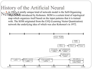
⚫ in 1982, A totally unique kind of network model is the Self-Organizing
Map (SOM) introduced by Kohonen. SOM is a certain kind of topological
map which organizes itself based on the input patterns that it is trained
with. The SOM originated from the LVQ (Learning Vector Quantization)
network the underlying idea of which was also Kohonen's in 1972.
7.
History of ArtificialNeural
Networks
Since then, research on artificial neural networks has
remained active, leading to many new network types, as
well as hybrid algorithms and hardware for neural
information processing.
8.
Artificial Neural Network
⚫Anartificial neural network consists of a pool of simple
processing units which communicate by sending signals
to each other over a large number of weighted
connections.
9.
Artificial Neural Network
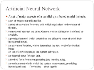
⚫A set of major aspects of a parallel distributed model include:
a set of processing units (cells).
a state of activation for every unit, which equivalent to the output of
the unit.
connections between the units. Generally each connection is defined by
a weight.
a propagation rule, which determines the effective input of a unit from
its external inputs.
an activation function, which determines the new level of activation
based
on the effective input and the current activation.
an external input for each unit.
a method for information gathering (the learning rule).
an environment within which the system must operate, providing
input signals and _ if necessary _ error signals.
10.
Computers vs. NeuralNetworks
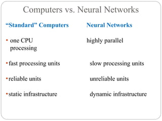
“Standard” Computers Neural Networks
⚫ one CPU highly parallel
processing
⚫fast processing units slow processing units
⚫reliable units unreliable units
⚫static infrastructure dynamic infrastructure
11.
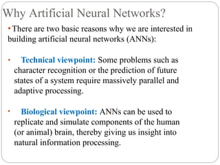
Why Artificial NeuralNetworks?
⚫There are two basic reasons why we are interested in
building artificial neural networks (ANNs):
• Technical viewpoint: Some problems such as
character recognition or the prediction of future
states of a system require massively parallel and
adaptive processing.
• Biological viewpoint: ANNs can be used to
replicate and simulate components of the human
(or animal) brain, thereby giving us insight into
natural information processing.
12.
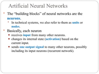
Artificial Neural Networks
•The “building blocks” of neural networks are the
neurons.
• In technical systems, we also refer to them as units or
nodes.
• Basically, each neuron
⚫ receives input from many other neurons.
⚫ changes its internal state (activation) based on the
current input.
⚫ sends one output signal to many other neurons, possibly
including its input neurons (recurrent network).
13.
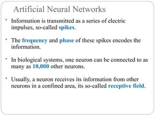
Artificial Neural Networks
•Information is transmitted as a series of electric
impulses, so-called spikes.
• The frequency and phase of these spikes encodes the
information.
• In biological systems, one neuron can be connected to as
many as 10,000 other neurons.
• Usually, a neuron receives its information from other
neurons in a confined area, its so-called receptive field.
14.
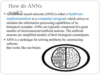
How do ANNs
work?
⚫An artificial neural network (ANN) is either a hardware
implementation or a computer program which strives to
simulate the information processing capabilities of its
biological exemplar. ANNs are typically composed of a great
number of interconnected artificial neurons. The artificial
neurons are simplified models of their biological counterparts.
⚫ ANN is a technique for solving problems by constructing
software
that works like our brains.
15.
How do ourbrains work?
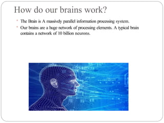
The Brain is A massively parallel information processing system.
Our brains are a huge network of processing elements. A typical brain
contains a network of 10 billion neurons.
16.
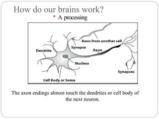
How do ourbrains work?
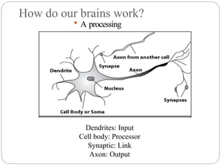
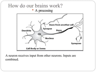
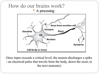
A processing
element
Dendrites: Input
Cell body: Processor
Synaptic: Link
Axon: Output
17.
How do ourbrains work?
A processing
element
A neuron is connected to other neurons through about
10,000 synapses
18.
How do ourbrains work?
A processing
element
A neuron receives input from other neurons. Inputs are
combined.
19.
How do ourbrains work?
A processing
element
Once input exceeds a critical level, the neuron discharges a spike
‐ an electrical pulse that travels from the body, down the axon, to
the next neuron(s)
20.
How do ourbrains work?
A processing
element
The axon endings almost touch the dendrites or cell body of
the next neuron.
21.
How do ourbrains work?
A processing
element
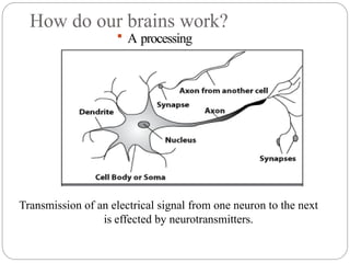
Transmission of an electrical signal from one neuron to the next
is effected by neurotransmitters.
22.
How do ourbrains work?
A processing
element
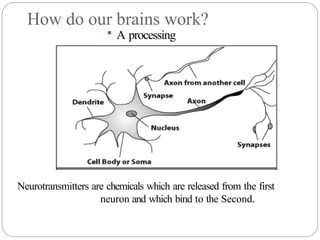
Neurotransmitters are chemicals which are released from the first
neuron and which bind to the Second.
23.
How do ourbrains work?
A processing
element
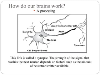
This link is called a synapse. The strength of the signal that
reaches the next neuron depends on factors such as the amount
of neurotransmitter available.
24.
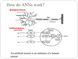
How do ANNswork?
An artificial neuron is an imitation of a human
neuron
25.
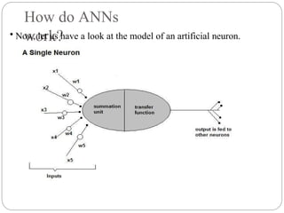
How do ANNs
work?
•Now, let us have a look at the model of an artificial neuron.
26.
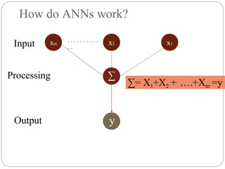
How do ANNswork?
Output
x1
x2
xm
∑
y
Processing
Input
∑= X1+X2 + ….+Xm =y
. . . . . . . . . .
. .
27.
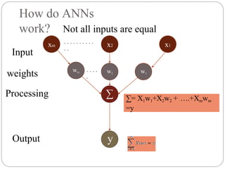
How do ANNs
work?Not all inputs are equal
Output
x1
xm x2
∑
y
Input
∑= X1w1+X2w2 + ….+Xmwm
=y
w1
w2
wm
weights
Processing
. . . . . . . . . .
. .
. . . .
.
28.
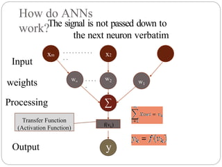
How do ANNs
work?Thesignal is not passed down to
the next neuron verbatim
Transfer Function
(Activation Function)
Output
xm x2
x1
∑
y
Input
w1
w2
wm
weights
Processing
. . . . . . . . . .
. .
f(vk)
. . . .
.
29.
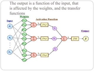
The output isa function of the input, that
is affected by the weights, and the transfer
functions
Artificial Neural Networks
⚫AnANN can:
1. compute any computable function, by the appropriate
selection of the network topology and weights values.
2. learn from experience!
Specifically, by trial and error
‐ ‐
32.
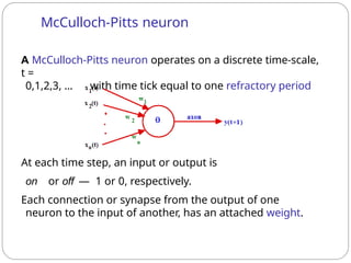
A McCulloch-Pitts neuronoperates on a discrete time-scale,
t =
0,1,2,3, ... with time tick equal to one refractory period
At each time step, an input or output is
on or off — 1 or 0, respectively.
Each connection or synapse from the output of one
neuron to the input of another, has an attached weight.
McCulloch-Pitts neuron
33.
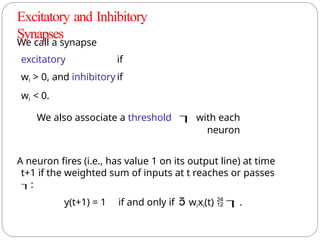
We call asynapse
excitatory if
wi > 0, and inhibitory if
wi < 0.
We also associate a threshold with each
neuron
A neuron fires (i.e., has value 1 on its output line) at time
t+1 if the weighted sum of inputs at t reaches or passes
:
y(t+1) = 1 if and only if wixi(t) .
Excitatory and Inhibitory
Synapses
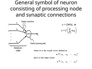
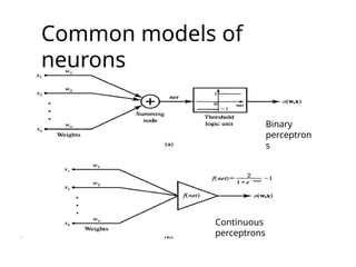
General symbol ofneuron
consisting of processing node
and synaptic connections
37.
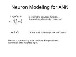
Neuron Modeling forANN
Is referred to activation function.
Domain is set of activation values net.
Scalar product of weight and input vector
Neuron as a processing node performs the operation of
summation of its weighted input.
38.
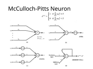
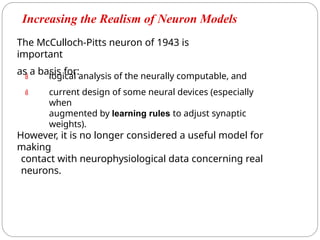
The McCulloch-Pitts neuronof 1943 is
important
as a basis for:
logical analysis of the neurally computable, and
current design of some neural devices (especially
when
augmented by learning rules to adjust synaptic
weights).
However, it is no longer considered a useful model for
making
contact with neurophysiological data concerning real
neurons.
Increasing the Realism of Neuron Models
39.
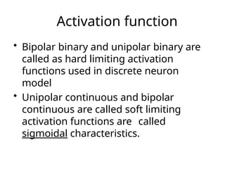
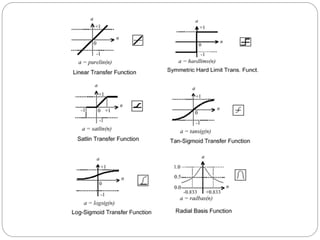
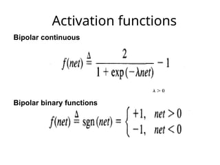
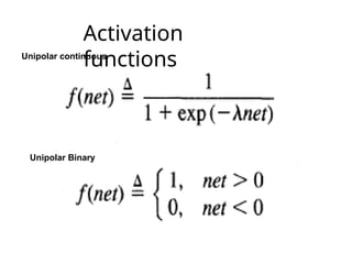
Activation function
• Bipolarbinary and unipolar binary are
called as hard limiting activation
functions used in discrete neuron
model
• Unipolar continuous and bipolar
continuous are called soft limiting
activation functions are called
sigmoidal characteristics.
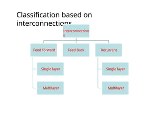
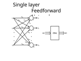
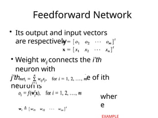
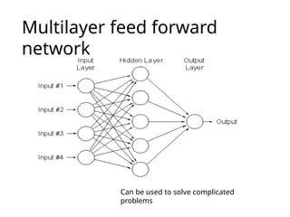
Feedforward Network
• Itsoutput and input vectors
are respectively
• Weight wij connects the i’th
neuron with
j’th input. Activation rule of ith
neuron is
wher
e
EXAMPLE
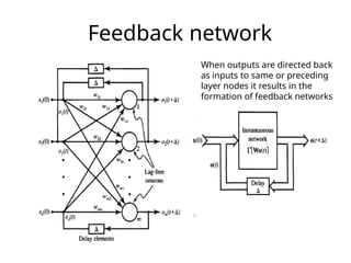
Feedback network
When outputsare directed back
as inputs to same or preceding
layer nodes it results in the
formation of feedback networks
49.
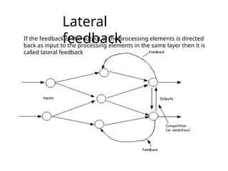
Lateral
feedback
If the feedbackof the output of the processing elements is directed
back as input to the processing elements in the same layer then it is
called lateral feedback
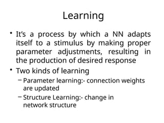
Learning
• It’s aprocess by which a NN adapts
itself to a stimulus by making proper
parameter adjustments, resulting in
the production of desired response
• Two kinds of learning
– Parameter learning:- connection weights
are updated
– Structure Learning:- change in
network structure
53.
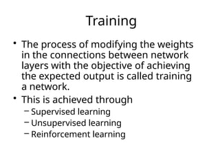
Training
• The processof modifying the weights
in the connections between network
layers with the objective of achieving
the expected output is called training
a network.
• This is achieved through
– Supervised learning
– Unsupervised learning
– Reinforcement learning
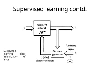
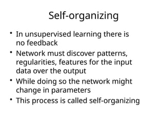
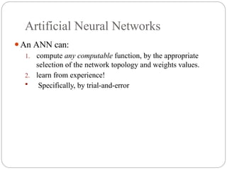
Supervised Learning
• Childlearns from a teacher
• Each input vector requires a Corresponding
target vector.
• Training pair=[input vector, target vector]
Neural
Networ
k W
Error
Signal
Generato
r
X
(Input
)
Y
(Actual
output)
(Desired
Output)
Error
(D-Y)
sign
als
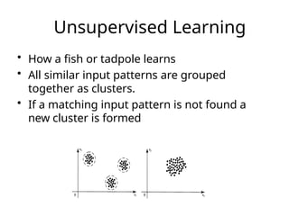
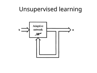
Unsupervised Learning
• Howa fish or tadpole learns
• All similar input patterns are grouped
together as clusters.
• If a matching input pattern is not found a
new cluster is formed
Self-organizing
• In unsupervisedlearning there is
no feedback
• Network must discover patterns,
regularities, features for the input
data over the output
• While doing so the network might
change in parameters
• This process is called self-organizing
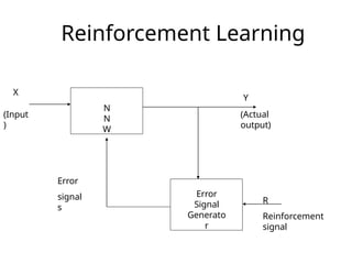
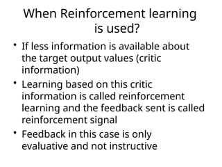
When Reinforcement learning
isused?
• If less information is available about
the target output values (critic
information)
• Learning based on this critic
information is called reinforcement
learning and the feedback sent is called
reinforcement signal
• Feedback in this case is only
evaluative and not instructive
62.
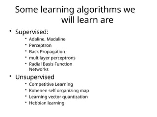
Some learning algorithmswe
will learn are
• Supervised:
• Adaline, Madaline
• Perceptron
• Back Propagation
• multilayer perceptrons
• Radial Basis Function
Networks
• Unsupervised
• Competitive Learning
• Kohenen self organizing map
• Learning vector quantization
• Hebbian learning
63.
Neural processing
• Recall:-processing phase for a NN and
its objective is to retrieve the
information. The process of computing
o for a given x
• Basic forms of neural information
processing
– Auto association
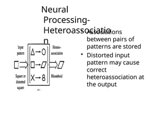
– Hetero association
– Classification
64.
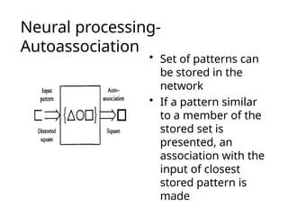
Neural processing-
Autoassociation
• Setof patterns can
be stored in the
network
• If a pattern similar
to a member of the
stored set is
presented, an
association with the
input of closest
stored pattern is
made
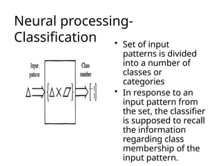
Neural processing-
Classification •Set of input
patterns is divided
into a number of
classes or
categories
• In response to an
input pattern from
the set, the classifier
is supposed to recall
the information
regarding class
membership of the
input pattern.
67.
Important terminologies of
ANNs
•Weights
• Bias
• Threshold
• Learning rate
• Momentum factor
• Vigilance parameter
• Notations used in
ANN
68.
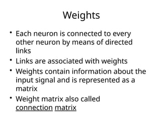
Weights
• Each neuronis connected to every
other neuron by means of directed
links
• Links are associated with weights
• Weights contain information about the
input signal and is represented as a
matrix
• Weight matrix also called
connection matrix
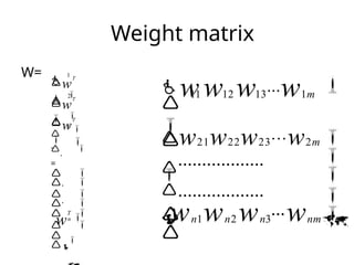
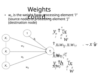
Weights
contd…
• wij –isthe weight from processing element ”i”
(source node) to processing element “j”
(destination node)
X1
1
Xi
Yj
Xn
w1j
wij
wnj
bj
n
i
0
i
ij
in
j
n
nj
n
n
i
1
j i
ij
in
j
y x
w
y
i
1
x0w0 j
x1w1 j
x2w2 j
.... x w
w0 j
xiwi
j
b x
w
71.
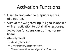
Activation Functions
• Usedto calculate the output response
of a neuron.
• Sum of the weighted input signal is applied
with an activation to obtain the response.
• Activation functions can be linear or non
linear
• Already dealt
– Identity function
– Single/binary step function
– Discrete/continuous sigmoidal function.
72.
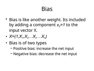
Bias
• Bias islike another weight. Its included
by adding a component x0=1 to the
input vector X.
• X=(1,X1,X2…Xi,…Xn)
• Bias is of two types
– Positive bias: increase the net input
– Negative bias: decrease the net input
73.
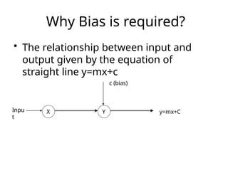
Why Bias isrequired?
X Y
• The relationship between input and
output given by the equation of
straight line y=mx+c
c (bias)
Inpu
t
y=mx+C
74.
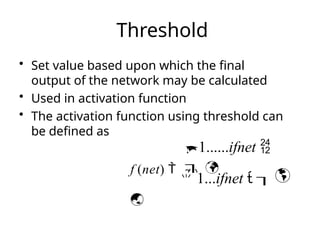
Threshold
• Set valuebased upon which the final
output of the network may be calculated
• Used in activation function
• The activation function using threshold can
be defined as
1......ifnet
f (net)
1...ifnet
75.
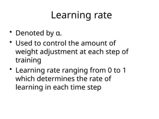
Learning rate
• Denotedby α.
• Used to control the amount of
weight adjustment at each step of
training
• Learning rate ranging from 0 to 1
which determines the rate of
learning in each time step
76.
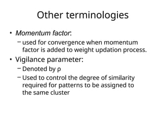
Other terminologies
• Momentumfactor:
– used for convergence when momentum
factor is added to weight updation process.
• Vigilance parameter:
– Denoted by ρ
– Used to control the degree of similarity
required for patterns to be assigned to
the same cluster


![Supervised Learning
• Child learns from a teacher
• Each input vector requires a Corresponding
target vector.
• Training pair=[input vector, target vector]
Neural
Networ
k W
Error
Signal
Generato
r
X
(Input
)
Y
(Actual
output)
(Desired
Output)
Error
(D-Y)
sign
als](https://image.slidesharecdn.com/publication319749213-250814092842-dd147144/85/publication_3_19749_213-publicationpublication-55-320.jpg)