Data Mining

1. Data Warehousing

2. Unit 1: Data Warehousing
• Data Warehousing: Overview, Definition
• Delivery Process
• Difference between Database System and Data Warehouse,
• Multi-Dimensional Data Model: Data Cubes, Stars and Snow
Flake Schema,
• Fact Constellations,
• Concept hierarchy,
• Process Architecture,
• 3 Tier Architecture,
• Data Mart, Slowly
• Changing Dimensions (SCD),
• OLAP: ROLAP, MOLAP, HOLAP.

3. History of Decision-Support Systems
Depending on the size and nature of the business, most companies have gone through
the following stages of attempts to provide strategic information for decision making:
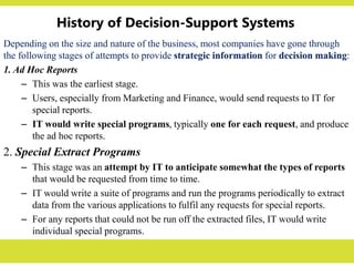
1. Ad Hoc Reports
– This was the earliest stage.
– Users, especially from Marketing and Finance, would send requests to IT for
special reports.
– IT would write special programs, typically one for each request, and produce
the ad hoc reports.
2. Special Extract Programs
– This stage was an attempt by IT to anticipate somewhat the types of reports
that would be requested from time to time.
– IT would write a suite of programs and run the programs periodically to extract
data from the various applications to fulfil any requests for special reports.
– For any reports that could not be run off the extracted files, IT would write
individual special programs.

4. History of Decision-Support Systems
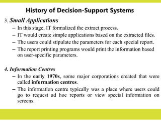
3. Small Applications
– In this stage, IT formalized the extract process.
– IT would create simple applications based on the extracted files.
– The users could stipulate the parameters for each special report.
– The report printing programs would print the information based
on user-specific parameters.
4. Information Centres
– In the early 1970s, some major corporations created that were
called information centres.
– The information centre typically was a place where users could
go to request ad hoc reports or view special information on
screens.

5. History of Decision-Support Systems
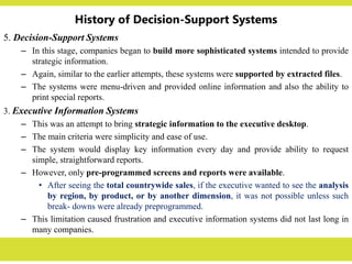
5. Decision-Support Systems
– In this stage, companies began to build more sophisticated systems intended to provide
strategic information.
– Again, similar to the earlier attempts, these systems were supported by extracted files.
– The systems were menu-driven and provided online information and also the ability to
print special reports.
3. Executive Information Systems
– This was an attempt to bring strategic information to the executive desktop.
– The main criteria were simplicity and ease of use.
– The system would display key information every day and provide ability to request
simple, straightforward reports.
– However, only pre-programmed screens and reports were available.
• After seeing the total countrywide sales, if the executive wanted to see the analysis
by region, by product, or by another dimension, it was not possible unless such
break- downs were already preprogrammed.
– This limitation caused frustration and executive information systems did not last long in
many companies.

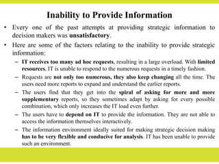
6. Inability to Provide Information
• Every one of the past attempts at providing strategic information to
decision makers was unsatisfactory.
• Here are some of the factors relating to the inability to provide strategic
information:
– IT receives too many ad hoc requests, resulting in a large overload. With limited
resources, IT is unable to respond to the numerous requests in a timely fashion.
– Requests are not only too numerous, they also keep changing all the time. The
users need more reports to expand and understand the earlier reports.
– The users find that they get into the spiral of asking for more and more
supplementary reports, so they sometimes adapt by asking for every possible
combination, which only increases the IT load even further.
– The users have to depend on IT to provide the information. They are not able to
access the information themselves interactively.
– The information environment ideally suited for making strategic decision making
has to be very flexible and conducive for analysis. IT has been unable to provide
such an environment.

7. 7
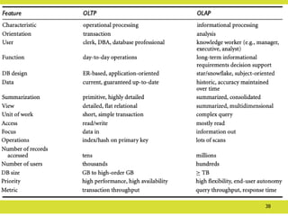
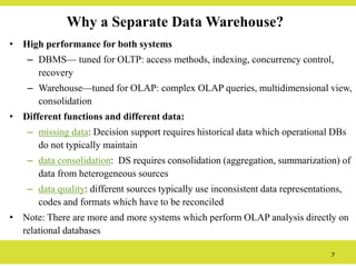
Why a Separate Data Warehouse?
• High performance for both systems
– DBMS— tuned for OLTP: access methods, indexing, concurrency control,
recovery
– Warehouse—tuned for OLAP: complex OLAP queries, multidimensional view,
consolidation
• Different functions and different data:
– missing data: Decision support requires historical data which operational DBs
do not typically maintain
– data consolidation: DS requires consolidation (aggregation, summarization) of
data from heterogeneous sources
– data quality: different sources typically use inconsistent data representations,
codes and formats which have to be reconciled
• Note: There are more and more systems which perform OLAP analysis directly on
relational databases

8. 8
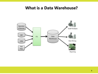
What is a Data Warehouse?
Operation
al Sources
ERP
CRM
Flat
Files
ETL Data
Warehouse
OLAP Analysis
Data Mining
Reporting

9. 9
What is a Data Warehouse?
• Data warehouses generalize and consolidate data in
multidimensional space.
• Data warehousing provides architectures and tools for
business executives to systematically organize,
understand, and use their data to make strategic
decisions.
• A decision support database that is maintained
separately from the organization’s operational database.
• Support information processing by providing a solid
platform of consolidated, historical data for analysis.

10. 10
What is a Data Warehouse?
• “Then, what exactly is a data warehouse?”
– Data warehouses have been defined in many ways,
making it difficult to formulate a rigorous definition.
– Loosely speaking, a data warehouse refers to a data
repository that is maintained separately from an
organization’s operational databases.
– Data warehouse systems allow for integration of a
variety of application systems.
– They support information processing by providing
a solid platform of consolidated historic data for
analysis.

11. 11
What is a Data Warehouse?
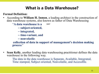
Formal Definition:
• According to William H. Inmon, a leading architect in the construction of
data warehouse systems, also known as father of Data Warehousing
“A data warehouse is a
– subject-oriented,
– integrated,
– time-variant, and
– nonvolatile
collection of data in support of management’s decision making
process”
• Sean Kelly, another leading data warehousing practitioner defines the data
warehouse in the following way.
The data in the data warehouse is Separate, Available, Integrated,
Time stamped, Subject oriented, Nonvolatile, and Accessible.
SINT

12. 12
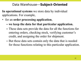
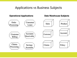
Data Warehouse—Subject-Oriented
In operational systems we store data by individual
applications. For example,
• for an order processing application,
– we keep the data for that particular application.
– These data sets provide the data for all the functions for
entering orders, checking stock, verifying customer’s
credit, and assigning the order for shipment.
– But these data sets contain only the data that is needed
for those functions relating to this particular application.

13. 13
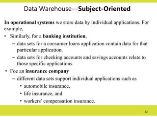
Data Warehouse—Subject-Oriented
In operational systems we store data by individual applications. For
example,
• Similarly, for a banking institution,
– data sets for a consumer loans application contain data for that
particular application.
– data sets for checking accounts and savings accounts relate to
those specific applications.
• Foe an insurance company
– different data sets support individual applications such as
• automobile insurance,
• life insurance, and
• workers’ compensation insurance.

14. 14
Data Warehouse—Subject-Oriented
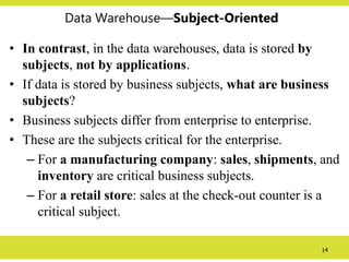
• In contrast, in the data warehouses, data is stored by
subjects, not by applications.
• If data is stored by business subjects, what are business
subjects?
• Business subjects differ from enterprise to enterprise.
• These are the subjects critical for the enterprise.
– For a manufacturing company: sales, shipments, and
inventory are critical business subjects.
– For a retail store: sales at the check-out counter is a
critical subject.

15. Applications vs Business Subjects

16. 16
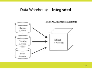
Data Warehouse—Integrated
• Constructed by integrating multiple, heterogeneous data
sources
– relational databases,
– flat files,
– on-line transaction records etc.
• Data cleaning and data integration techniques are applied.
– Ensure consistency in naming conventions, encoding
structures, attribute measures, etc. among different data
sources
• E.g., Hotel price: currency, tax, breakfast covered,
etc.
– When data is moved to the warehouse, it is converted.

17. 17
Data Warehouse—Integrated

18. 18
Data Warehouse—Time Variant
• The time horizon for the data warehouse is significantly longer than
that of operational systems
– Operational database: current value data (day-to-day current
operations).
– Data warehouse data: provide information from a historical
perspective (e.g., past 5-10 years)
• Every key structure in the data warehouse
– Contains an element of time, explicitly or implicitly
– But the key of operational data may or may not contain “time
element”
• The time-variant nature of the data in a data warehouse
– Allows for analysis of the past
– Relates information to the present
– Enables forecasts for the future

19. 19
Data Warehouse—Nonvolatile
• A physically separate store of data transformed from
the operational environment
• Operational update of data does not occur in the
data warehouse environment
– Does not require transaction processing, recovery,
and concurrency control mechanisms
– Requires only two operations in data accessing:
• initial loading of data and access of data

20. 20
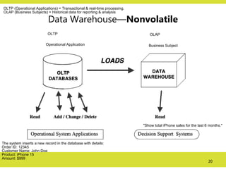
Data Warehouse—Nonvolatile
Operational Application Business Subject
OLTP OLAP
"Show total iPhone sales for the last 6 months."
The system inserts a new record in the database with details:
Order ID: 12345
Customer Name: John Doe
Product: iPhone 15
Amount: $999
OLTP (Operational Applications) = Transactional & real-time processing.
OLAP (Business Subjects) = Historical data for reporting & analysis

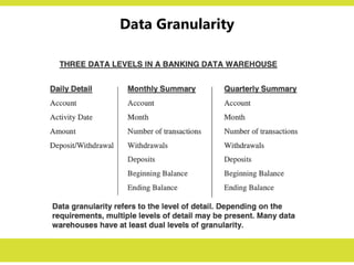
21. Data Granularity
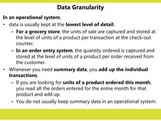
In an operational system,
• data is usually kept at the lowest level of detail.
– For a grocery store, the units of sale are captured and stored at
the level of units of a product per transaction at the check-out
counter.
– In an order entry system, the quantity ordered is captured and
stored at the level of units of a product per order received from
the customer.
• Whenever you need summary data, you add up the individual
transactions.
– If you are looking for units of a product ordered this month,
you read all the orders entered for the entire month for that
product and add up.
– You do not usually keep summary data in an operational system.

22. Data Granularity
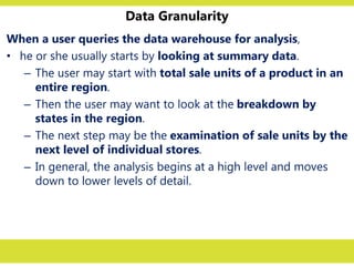
When a user queries the data warehouse for analysis,
• he or she usually starts by looking at summary data.
– The user may start with total sale units of a product in an
entire region.
– Then the user may want to look at the breakdown by
states in the region.
– The next step may be the examination of sale units by the
next level of individual stores.
– In general, the analysis begins at a high level and moves
down to lower levels of detail.

23. Data Granularity
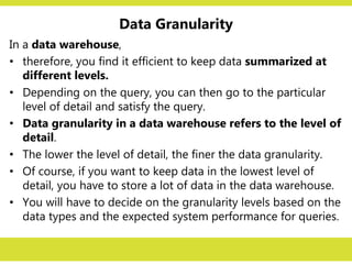
In a data warehouse,
• therefore, you find it efficient to keep data summarized at
different levels.
• Depending on the query, you can then go to the particular
level of detail and satisfy the query.
• Data granularity in a data warehouse refers to the level of
detail.
• The lower the level of detail, the finer the data granularity.
• Of course, if you want to keep data in the lowest level of
detail, you have to store a lot of data in the data warehouse.
• You will have to decide on the granularity levels based on the
data types and the expected system performance for queries.

24. Data Granularity

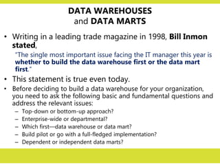
25. DATA WAREHOUSES
and DATA MARTS
• Writing in a leading trade magazine in 1998, Bill Inmon
stated,
“The single most important issue facing the IT manager this year is
whether to build the data warehouse first or the data mart
first.”
• This statement is true even today.
• Before deciding to build a data warehouse for your organization,
you need to ask the following basic and fundamental questions and
address the relevant issues:
– Top-down or bottom-up approach?
– Enterprise-wide or departmental?
– Which first—data warehouse or data mart?
– Build pilot or go with a full-fledged implementation?
– Dependent or independent data marts?

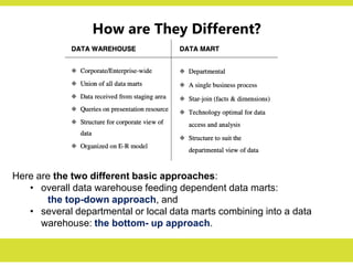
26. How are They Different?
Here are the two different basic approaches:
• overall data warehouse feeding dependent data marts:
the top-down approach, and
• several departmental or local data marts combining into a data
warehouse: the bottom- up approach.

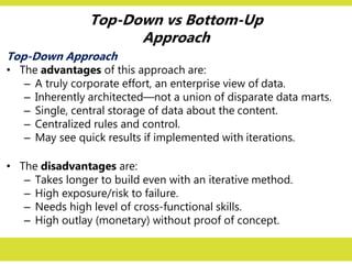
27. Top-Down vs Bottom-Up
Approach
Top-Down Approach
• The advantages of this approach are:
– A truly corporate effort, an enterprise view of data.
– Inherently architected—not a union of disparate data marts.
– Single, central storage of data about the content.
– Centralized rules and control.
– May see quick results if implemented with iterations.
• The disadvantages are:
– Takes longer to build even with an iterative method.
– High exposure/risk to failure.
– Needs high level of cross-functional skills.
– High outlay (monetary) without proof of concept.

28. Top-Down vs Bottom-Up
Approach
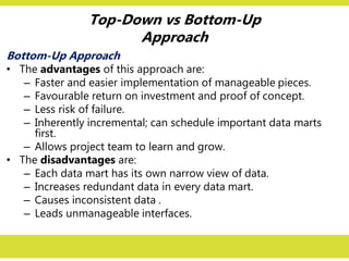
Bottom-Up Approach
• The advantages of this approach are:
– Faster and easier implementation of manageable pieces.
– Favourable return on investment and proof of concept.
– Less risk of failure.
– Inherently incremental; can schedule important data marts
first.
– Allows project team to learn and grow.
• The disadvantages are:
– Each data mart has its own narrow view of data.
– Increases redundant data in every data mart.
– Causes inconsistent data .
– Leads unmanageable interfaces.

29. A Practical Approach
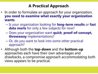
• In order to formulate an approach for your organization,
you need to examine what exactly your organization
wants.
– Is your organization looking for long-term results or fast
data marts for only a few subjects for now?
– Does your organization want quick, proof-of-concept,
throwaway implementations?
– Or, do you want to look into some other practical
approach?
• Although both the top-down and the bottom-up
approaches each have their own advantages and
drawbacks, a compromise approach accommodating both
views appears to be practical.

30. A Practical Approach
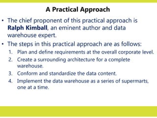
• The chief proponent of this practical approach is
Ralph Kimball, an eminent author and data
warehouse expert.
• The steps in this practical approach are as follows:
1. Plan and define requirements at the overall corporate level.
2. Create a surrounding architecture for a complete
warehouse.
3. Conform and standardize the data content.
4. Implement the data warehouse as a series of supermarts,
one at a time.

31. 31
Three Data Warehouse Models
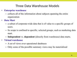
• Enterprise warehouse
– collects all of the information about subjects spanning the entire
organization
• Data Mart
– a subset of corporate-wide data that is of value to a specific groups of
users.
– Its scope is confined to specific, selected groups, such as marketing data
mart.
– Independent vs. dependent (directly from warehouse) data marts.
• Virtual warehouse
– A set of views over operational databases
– Only some of the possible summary views may be materialized

32. 32
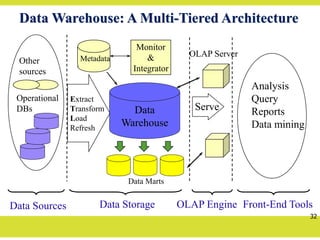
Data Warehouse: A Multi-Tiered Architecture
Data
Warehouse
Extract
Transform
Load
Refresh
OLAP Engine
Analysis
Query
Reports
Data mining
Monitor
&
Integrator
Metadata
Data Sources Front-End Tools
Serve
Data Marts
Operational
DBs
Other
sources
Data Storage
OLAP Server

33. 33
Data Sources
• Source data coming into the data warehouse may be grouped
into four broad categories, as discussed here.
– Production Data: This category of data comes from the
various operational systems of the enterprise.
– Internal Data: In every organization, users keep their
“private” spreadsheets, documents, customer profiles, and
sometimes even departmental databases. This is the internal
data, parts of which could be useful in a data warehouse.
– Archived Data: In every operational system, you periodically
take the old data and store it in archived files.
– External Data: Most executives depend on data from
external sources for a high percentage of the information they
use. They use statistics relating to their industry produced by
external agencies or market share data of competitors.

34. 34
Extraction,
Transformation, and Loading (ETL)
• Data extraction
– get data from multiple, heterogeneous, and external sources
• Data cleaning
– detect errors in the data and rectify them when possible
• Data transformation
– convert data from legacy or host format to warehouse format
• Load
– sort, summarize, consolidate, compute views, check integrity,
and build indicies and partitions
• Refresh
– propagate the updates from the data sources to the warehouse

35. 35
Metadata Repository
Metadata is the data defining warehouse objects.
It stores:
• Description of the structure of the data warehouse
– schema, view, dimensions, hierarchies, derived data definitions, data mart
locations and contents
• Operational metadata
– data lineage (history of migrated data and transformation path),
– currency of data (active, archived, or purged),
– monitoring information (warehouse usage statistics, error reports, audit trails)
• The algorithms used for summarization
• The mapping from operational environment to the data warehouse
• Data related to system performance
– warehouse schema, view and derived data definitions
• Business data
– business terms and definitions, ownership of data, charging policies

36. OnLine Analytical Processing (OLAP)
• An OLAP tool enables analysts, managers, and decision makers to gain insights
into data through fast, consistent, interactive access to a variety of possible views
of information transformed from raw data to reflect real dimensionality of the
enterprise as understood by the users.
• OLAP is used for analysis of data because it enables
• Multidimensional analysis
• Fast access
• Powerful calculations
like:
 Summaries and Aggregation,
 Moving from summaries to detailed and vice-versa,
 Simple Calculations,
 Shared Calculation,
 Trend analysis using statistical methods etc.
Read: OLAP Council White Paper, 1997,
URL: http://www.olapcouncil.org/research/whtpaply.htm

37. OLAP Query
 A sequence of OLAP queries is required for an analysis session.
 The OLAP queries can be in SQL or MDX (MultiDimensional
eXpression) query languages depending on the OLAP tools.
MDX Query sample:
Query1:
select Crossjoin({[Time].[Month].Members}, {[Measures].[Store Cost]}) ON COLUMNS,
{[Store].[Mexico]} ON ROWS
from [Sales]
Query2:
select Crossjoin(Crossjoin({[Time].[Month].Members}, {[Store Type].[Store Type].Members}),
{[Measures].[Sales Count]}) ON COLUMNS,
{[Store Size in SQFT].[24597]} ON ROWS
from [Sales]

38. 38

39. 39
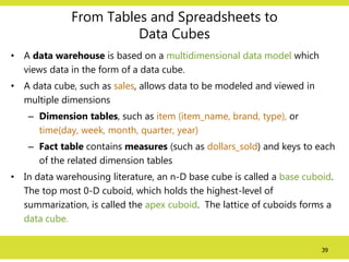
From Tables and Spreadsheets to
Data Cubes
• A data warehouse is based on a multidimensional data model which
views data in the form of a data cube.
• A data cube, such as sales, allows data to be modeled and viewed in
multiple dimensions
– Dimension tables, such as item (item_name, brand, type), or
time(day, week, month, quarter, year)
– Fact table contains measures (such as dollars_sold) and keys to each
of the related dimension tables
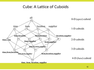
• In data warehousing literature, an n-D base cube is called a base cuboid.
The top most 0-D cuboid, which holds the highest-level of
summarization, is called the apex cuboid. The lattice of cuboids forms a
data cube.

40. 40
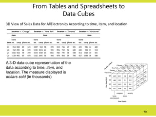
From Tables and Spreadsheets to
Data Cubes
3D View of Sales Data for AllElectronics According to time, item, and location
A 3-D data cube representation of the
data according to time, item, and
location. The measure displayed is
dollars sold (in thousands)

41. 41
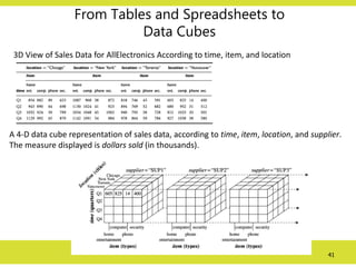
From Tables and Spreadsheets to
Data Cubes
3D View of Sales Data for AllElectronics According to time, item, and location
A 4-D data cube representation of sales data, according to time, item, location, and supplier.
The measure displayed is dollars sold (in thousands).

42. 42
Cube: A Lattice of Cuboids
time,item
time,item,location
time, item, location, supplier
all
time item location supplier
time,location
time,supplier
item,location
item,supplier
location,supplier
time,item,supplier
time,location,supplier
item,location,supplier
0-D (apex) cuboid
1-D cuboids
2-D cuboids
3-D cuboids
4-D (base) cuboid

43. 43
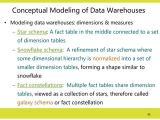
Conceptual Modeling of Data Warehouses
• Modeling data warehouses: dimensions & measures
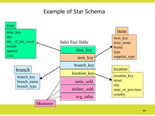
– Star schema: A fact table in the middle connected to a set
of dimension tables
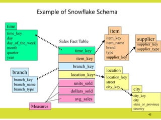
– Snowflake schema: A refinement of star schema where
some dimensional hierarchy is normalized into a set of
smaller dimension tables, forming a shape similar to
snowflake
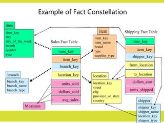
– Fact constellations: Multiple fact tables share dimension
tables, viewed as a collection of stars, therefore called
galaxy schema or fact constellation

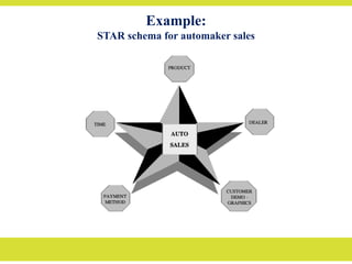
44. 44
Example of Star Schema
time_key
day
day_of_the_week
month
quarter
year
time
location_key
street
city
state_or_province
country
location
Sales Fact Table
time_key
item_key
branch_key
location_key
units_sold
dollars_sold
avg_sales
Measures
item_key
item_name
brand
type
supplier_type
item
branch_key
branch_name
branch_type
branch

45. 45
Example of Snowflake Schema
time_key
day
day_of_the_week
month
quarter
year
time
location_key
street
city_key
location
Sales Fact Table
time_key
item_key
branch_key
location_key
units_sold
dollars_sold
avg_sales
Measures
item_key
item_name
brand
type
supplier_key
item
branch_key
branch_name
branch_type
branch
supplier_key
supplier_type
supplier
city_key
city
state_or_province
country
city

46. 46
Example of Fact Constellation
time_key
day
day_of_the_week
month
quarter
year
time
location_key
street
city
province_or_state
country
location
Sales Fact Table
time_key
item_key
branch_key
location_key
units_sold
dollars_sold
avg_sales
Measures
item_key
item_name
brand
type
supplier_type
item
branch_key
branch_name
branch_type
branch
Shipping Fact Table
time_key
item_key
shipper_key
from_location
to_location
dollars_cost
units_shipped
shipper_key
shipper_name
location_key
shipper_type
shipper

47. 47
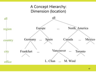
A Concept Hierarchy:
Dimension (location)
all
Europe North_America
Mexico
Canada
Spain
Germany
Vancouver
M. Wind
L. Chan
...
...
...
... ...
...
all
region
office
country
Toronto
Frankfurt
city

48. 48
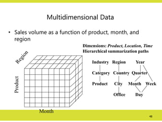
Multidimensional Data
• Sales volume as a function of product, month, and
region
Product
Month
Dimensions: Product, Location, Time
Hierarchical summarization paths
Industry Region Year
Category Country Quarter
Product City Month Week
Office Day

49. 49
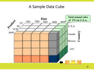
A Sample Data Cube
Total annual sales
of TVs in U.S.A.
Date
Country
sum
sum
TV
VCR
PC
1Qtr 2Qtr 3Qtr 4Qtr
U.S.A
Canada
Mexico
sum

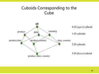
50. 50
Cuboids Corresponding to the
Cube
all
product date country
product,date product,country date, country
product, date, country
0-D (apex) cuboid
1-D cuboids
2-D cuboids
3-D (base) cuboid

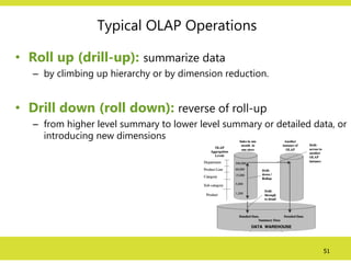
51. 51
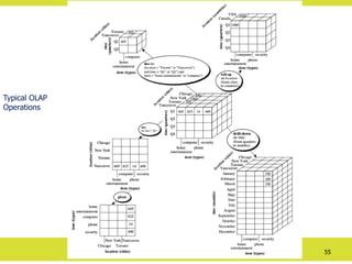
Typical OLAP Operations
• Roll up (drill-up): summarize data
– by climbing up hierarchy or by dimension reduction.
• Drill down (roll down): reverse of roll-up
– from higher level summary to lower level summary or detailed data, or
introducing new dimensions

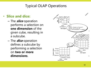
52. 52
Typical OLAP Operations
• Slice and dice:
– The slice operation
performs a selection on
one dimension of the
given cube, resulting in
a subcube.
– The dice operation
defines a subcube by
performing a selection
on two or more
dimensions.

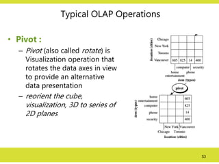
53. 53
Typical OLAP Operations
• Pivot :
– Pivot (also called rotate) is
Visualization operation that
rotates the data axes in view
to provide an alternative
data presentation
– reorient the cube,
visualization, 3D to series of
2D planes

54. 54
Typical OLAP Operations
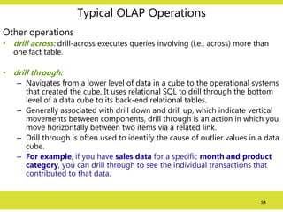
Other operations
• drill across: drill-across executes queries involving (i.e., across) more than
one fact table.
• drill through:
– Navigates from a lower level of data in a cube to the operational systems
that created the cube. It uses relational SQL to drill through the bottom
level of a data cube to its back-end relational tables.
– Generally associated with drill down and drill up, which indicate vertical
movements between components, drill through is an action in which you
move horizontally between two items via a related link.
– Drill through is often used to identify the cause of outlier values in a data
cube.
– For example, if you have sales data for a specific month and product
category, you can drill through to see the individual transactions that
contributed to that data.

55. 55
Typical OLAP
Operations

56. 56
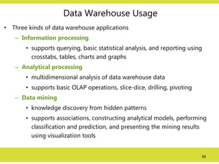
Data Warehouse Usage
• Three kinds of data warehouse applications
– Information processing
• supports querying, basic statistical analysis, and reporting using
crosstabs, tables, charts and graphs
– Analytical processing
• multidimensional analysis of data warehouse data
• supports basic OLAP operations, slice-dice, drilling, pivoting
– Data mining
• knowledge discovery from hidden patterns
• supports associations, constructing analytical models, performing
classification and prediction, and presenting the mining results
using visualization tools

57. 57
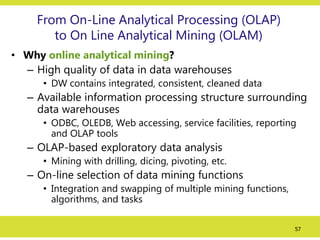
From On-Line Analytical Processing (OLAP)
to On Line Analytical Mining (OLAM)
• Why online analytical mining?
– High quality of data in data warehouses
• DW contains integrated, consistent, cleaned data
– Available information processing structure surrounding
data warehouses
• ODBC, OLEDB, Web accessing, service facilities, reporting
and OLAP tools
– OLAP-based exploratory data analysis
• Mining with drilling, dicing, pivoting, etc.
– On-line selection of data mining functions
• Integration and swapping of multiple mining functions,
algorithms, and tasks

58. 58
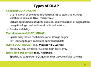
Types of OLAP
• Relational OLAP (ROLAP)
– Use relational or extended-relational DBMS to store and manage
warehouse data and OLAP middle ware
– Include optimization of DBMS backend, implementation of aggregation
navigation logic, and additional tools and services
– Greater scalability
• Multidimensional OLAP (MOLAP)
– Sparse array-based multidimensional storage engine
– Fast indexing to pre-computed summarized data
• Hybrid OLAP (HOLAP) (e.g., Microsoft SQLServer)
– Flexibility, e.g., low level: relational, high-level: array
• Specialized SQL servers (e.g., Redbricks)
– Specialized support for SQL queries over star/snowflake schemas

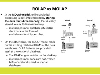
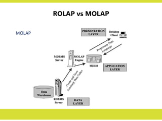
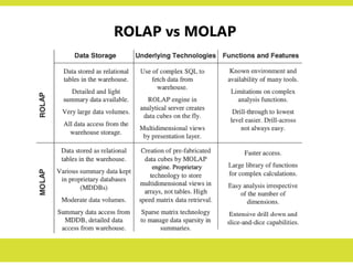
59. ROLAP vs MOLAP
• In the MOLAP model, online analytical
processing is best implemented by storing
the data multidimensionally, that is, easily
viewed in a multidimensional way.
– multidimensional databases (MDDBs)
store data in the form of
multidimensional hypercubes.
• On the other hand, the ROLAP model relies
on the existing relational DBMS of the data
warehouse. OLAP features are provided
against the relational database.
– The OLAP engine resides on the desktop.
– multidimensional cubes are not created
beforehand and stored in special
databases.

60. ROLAP vs MOLAP
MOLAP

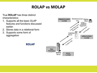
61. ROLAP
True ROLAP has three distinct
characteristics:
1. Supports all the basic OLAP
features and functions discussed
earlier.
2. Stores data in a relational form
3. Supports some form of
aggregation
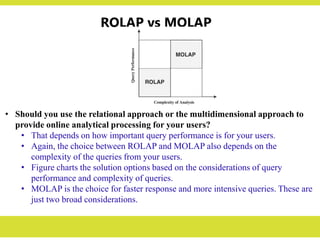
ROLAP vs MOLAP

62. ROLAP vs MOLAP

63. ROLAP vs MOLAP
• Should you use the relational approach or the multidimensional approach to
provide online analytical processing for your users?
• That depends on how important query performance is for your users.
• Again, the choice between ROLAP and MOLAP also depends on the
complexity of the queries from your users.
• Figure charts the solution options based on the considerations of query
performance and complexity of queries.
• MOLAP is the choice for faster response and more intensive queries. These are
just two broad considerations.

64. 64
64
DIMENSIONAL MODELING
DW Schema Design

65. FROM REQUIREMENTS TO
DATA DESIGN

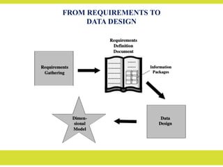
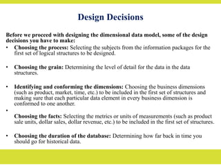
66. Design Decisions
Before we proceed with designing the dimensional data model, some of the design
decisions you have to make:
• Choosing the process: Selecting the subjects from the information packages for the
first set of logical structures to be designed.
• Choosing the grain: Determining the level of detail for the data in the data
structures.
• Identifying and conforming the dimensions: Choosing the business dimensions
(such as product, market, time, etc.) to be included in the first set of structures and
making sure that each particular data element in every business dimension is
conformed to one another.
•
Choosing the facts: Selecting the metrics or units of measurements (such as product
sale units, dollar sales, dollar revenue, etc.) to be included in the first set of structures.
• Choosing the duration of the database: Determining how far back in time you
should go for historical data.

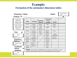
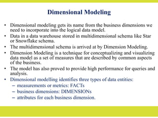
67. Dimensional Modeling
• Dimensional modeling gets its name from the business dimensions we
need to incorporate into the logical data model.
• Data in a data warehouse stored in multidimensional schema like Star
or Snowflake schema.
• The multidimensional schema is arrived at by Dimension Modeling.
• Dimension Modeling is a technique for conceptualizing and visualizing
data model as a set of measures that are described by common aspects
of the business.
• The model has also proved to provide high performance for queries and
analysis.
• Dimensional modelling identifies three types of data entities:
– measurements or metrics: FACTs
– business dimensions: DIMENSIONs
– attributes for each business dimension.

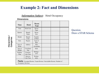
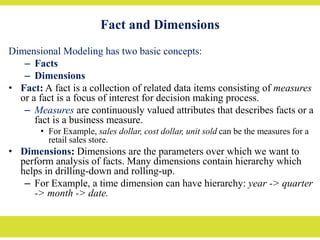
68. Fact and Dimensions
Dimensional Modeling has two basic concepts:
– Facts
– Dimensions
• Fact: A fact is a collection of related data items consisting of measures
or a fact is a focus of interest for decision making process.
– Measures are continuously valued attributes that describes facts or a
fact is a business measure.
• For Example, sales dollar, cost dollar, unit sold can be the measures for a
retail sales store.
• Dimensions: Dimensions are the parameters over which we want to
perform analysis of facts. Many dimensions contain hierarchy which
helps in drilling-down and rolling-up.
– For Example, a time dimension can have hierarchy: year -> quarter
-> month -> date.

69. Example:
Fact and Dimensions

70. Example:
Formation of the automaker dimension tables

71. Example:
STAR schema for automaker sales

72. Example 2: Fact and Dimensions
Question.
Draw a STAR Schema

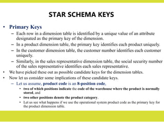
73. STAR SCHEMA KEYS
• Primary Keys
– Each row in a dimension table is identified by a unique value of an attribute
designated as the primary key of the dimension.
– In a product dimension table, the primary key identifies each product uniquely.
– In the customer dimension table, the customer number identifies each customer
uniquely.
– Similarly, in the sales representative dimension table, the social security number
of the sales representative identifies each sales representative.
• We have picked these out as possible candidate keys for the dimension tables.
• Now let us consider some implications of these candidate keys.
– Let us assume, product code is an 8-position code,
• two of which positions indicate the code of the warehouse where the product is normally
stored, and
• two other positions denote the product category.
• Let us see what happens if we use the operational system product code as the primary key for
the product dimension table.

74. STAR SCHEMA KEYS
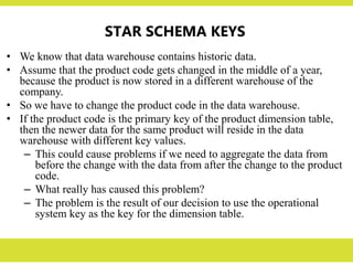
• We know that data warehouse contains historic data.
• Assume that the product code gets changed in the middle of a year,
because the product is now stored in a different warehouse of the
company.
• So we have to change the product code in the data warehouse.
• If the product code is the primary key of the product dimension table,
then the newer data for the same product will reside in the data
warehouse with different key values.
– This could cause problems if we need to aggregate the data from
before the change with the data from after the change to the product
code.
– What really has caused this problem?
– The problem is the result of our decision to use the operational
system key as the key for the dimension table.

75. STAR SCHEMA KEYS
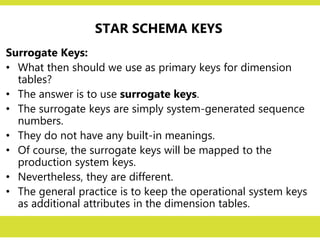
Surrogate Keys:
• What then should we use as primary keys for dimension
tables?
• The answer is to use surrogate keys.
• The surrogate keys are simply system-generated sequence
numbers.
• They do not have any built-in meanings.
• Of course, the surrogate keys will be mapped to the
production system keys.
• Nevertheless, they are different.
• The general practice is to keep the operational system keys
as additional attributes in the dimension tables.

76. Factless Fact Table

77. Factless Fact Table
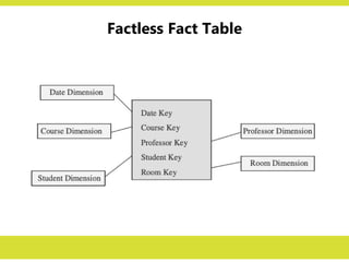
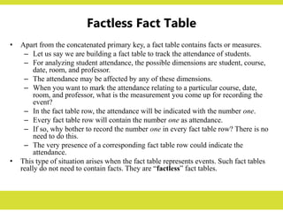
• Apart from the concatenated primary key, a fact table contains facts or measures.
– Let us say we are building a fact table to track the attendance of students.
– For analyzing student attendance, the possible dimensions are student, course,
date, room, and professor.
– The attendance may be affected by any of these dimensions.
– When you want to mark the attendance relating to a particular course, date,
room, and professor, what is the measurement you come up for recording the
event?
– In the fact table row, the attendance will be indicated with the number one.
– Every fact table row will contain the number one as attendance.
– If so, why bother to record the number one in every fact table row? There is no
need to do this.
– The very presence of a corresponding fact table row could indicate the
attendance.
• This type of situation arises when the fact table represents events. Such fact tables
really do not need to contain facts. They are “factless” fact tables.

78. E-R Modeling vs Dimensional
Modeling
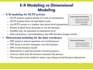
• E-R modeling for OLTP systems
– OLTP systems capture details of events or transactions
– OLTP systems focus on individual events
– An OLTP system is a window into micro-level transactions
– Picture at detail level necessary to run the business
– Suitable only for questions at transaction level
– Data consistency, non-redundancy, and efficient data storage critical.
• Dimensional modeling for the data warehouse.
– DW meant to answer questions on overall process
– DW focus is on how managers view the business
– DW reveals business trends
– Information is centered around a business process
– Answers show how the business measures the process
– The measures to be studied in many ways along several business dimensions

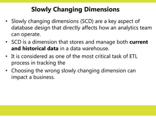
79. Slowly Changing Dimensions
• Slowly changing dimensions (SCD) are a key aspect of
database design that directly affects how an analytics team
can operate.
• SCD is a dimension that stores and manage both current
and historical data in a data warehouse.
• It is considered as one of the most critical task of ETL
process in tracking the
• Choosing the wrong slowly changing dimension can
impact a business.

80. Types of SCDs
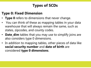
Type 0: Fixed Dimension
• Type 0 refers to dimensions that never change.
• You can think of these as mapping tables in your data
warehouse that will always remain the same, such as
states, zipcodes, and county codes.
• Date_dim tables that you may use to simplify joins are
also considers type 0 dimensions.
• In addition to mapping tables, other pieces of data like
social security number and date of birth are
considered type 0 dimensions.

81. Types of SCDs
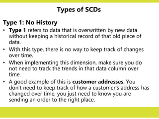
Type 1: No History
• Type 1 refers to data that is overwritten by new data
without keeping a historical record of that old piece of
data.
• With this type, there is no way to keep track of changes
over time.
• When implementing this dimension, make sure you do
not need to track the trends in that data column over
time.
• A good example of this is customer addresses. You
don’t need to keep track of how a customer’s address has
changed over time, you just need to know you are
sending an order to the right place.

82. Types of SCDs
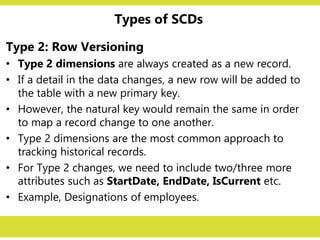
Type 2: Row Versioning
• Type 2 dimensions are always created as a new record.
• If a detail in the data changes, a new row will be added to
the table with a new primary key.
• However, the natural key would remain the same in order
to map a record change to one another.
• Type 2 dimensions are the most common approach to
tracking historical records.
• For Type 2 changes, we need to include two/three more
attributes such as StartDate, EndDate, IsCurrent etc.
• Example, Designations of employees.

83. Types of SCDs
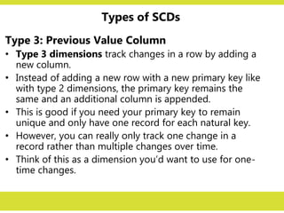
Type 3: Previous Value Column
• Type 3 dimensions track changes in a row by adding a
new column.
• Instead of adding a new row with a new primary key like
with type 2 dimensions, the primary key remains the
same and an additional column is appended.
• This is good if you need your primary key to remain
unique and only have one record for each natural key.
• However, you can really only track one change in a
record rather than multiple changes over time.
• Think of this as a dimension you’d want to use for one-
time changes.

84. Types of SCDs
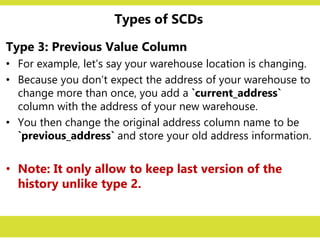
Type 3: Previous Value Column
• For example, let’s say your warehouse location is changing.
• Because you don’t expect the address of your warehouse to
change more than once, you add a `current_address`
column with the address of your new warehouse.
• You then change the original address column name to be
`previous_address` and store your old address information.
• Note: It only allow to keep last version of the
history unlike type 2.

85. Types of SCDs
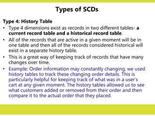
Type 4: History Table
• Type 4 dimensions exist as records in two different tables- a
current record table and a historical record table.
• All of the records that are active in a given moment will be in
one table and then all of the records considered historical will
exist in a separate history table.
• This is a great way of keeping track of records that have many
changes over time.
• Example: Order information may constantly changing, we used
history tables to track these changing order details. This is
particularly helpful for keeping track of what was in a user’s
cart at any given moment. The history tables allowed us to see
what customers added or removed from their order and then
compare it to the actual order that they placed.

86. Types of SCDs
Type 6: Hybrid of Type 1, Type 2 and Type 3
• Here we need to maintain a history of all changes,
simultaneously updating the “current value” columns on
all records