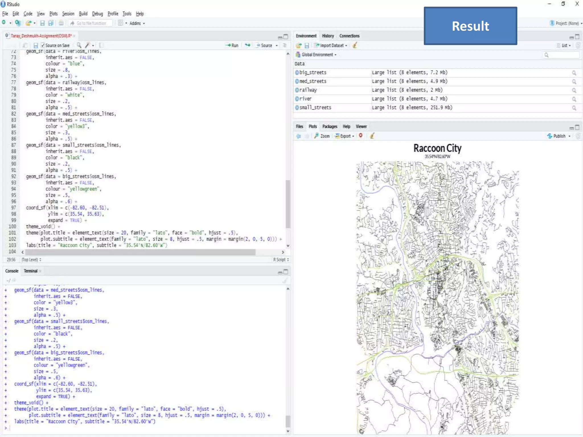
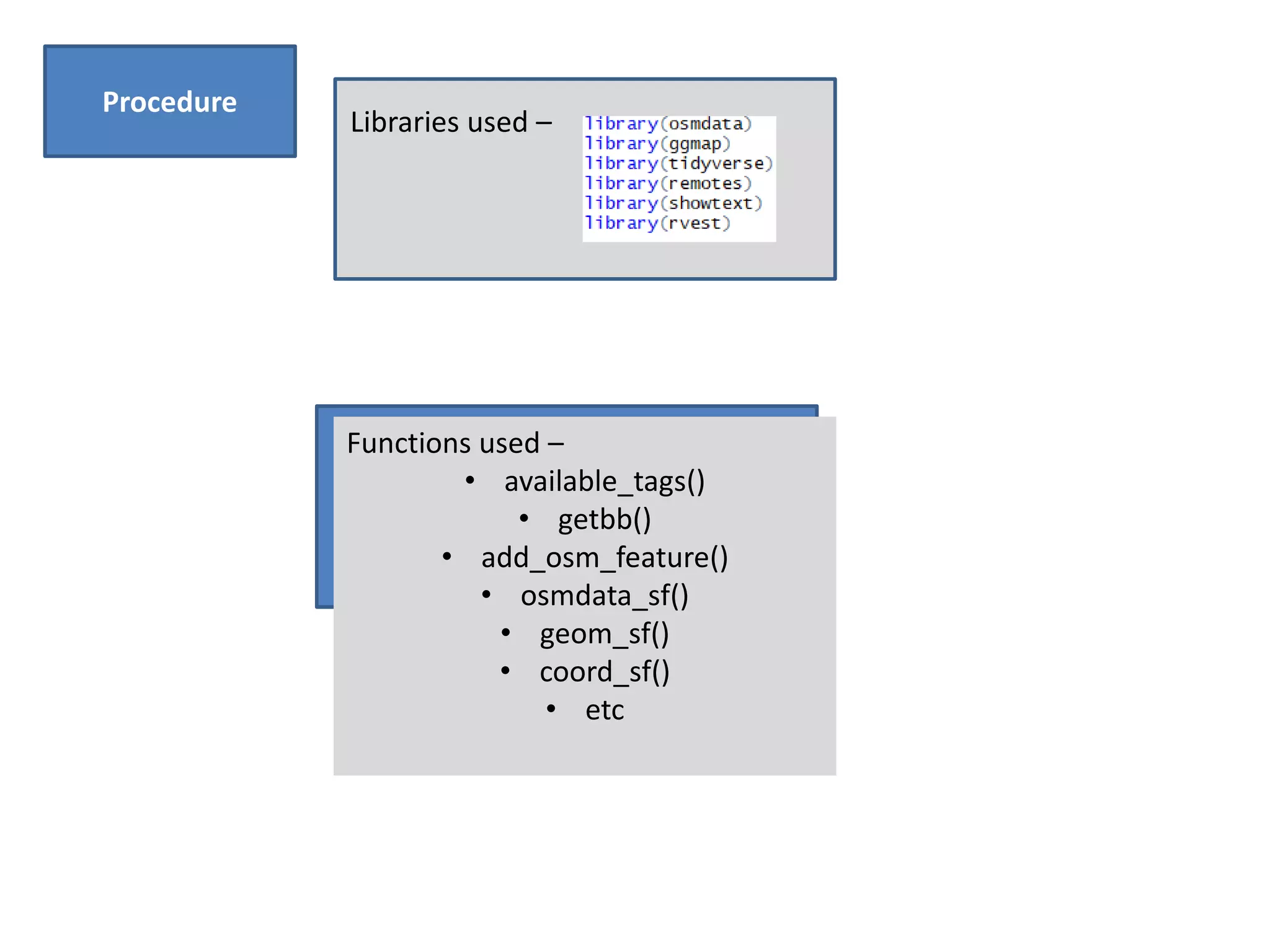
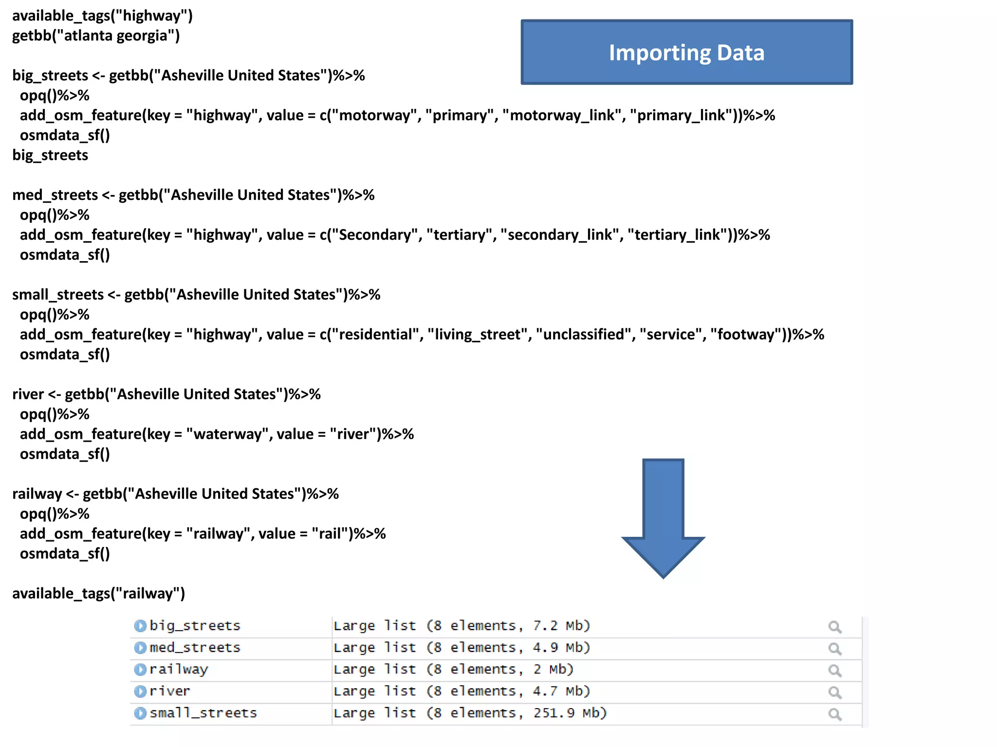
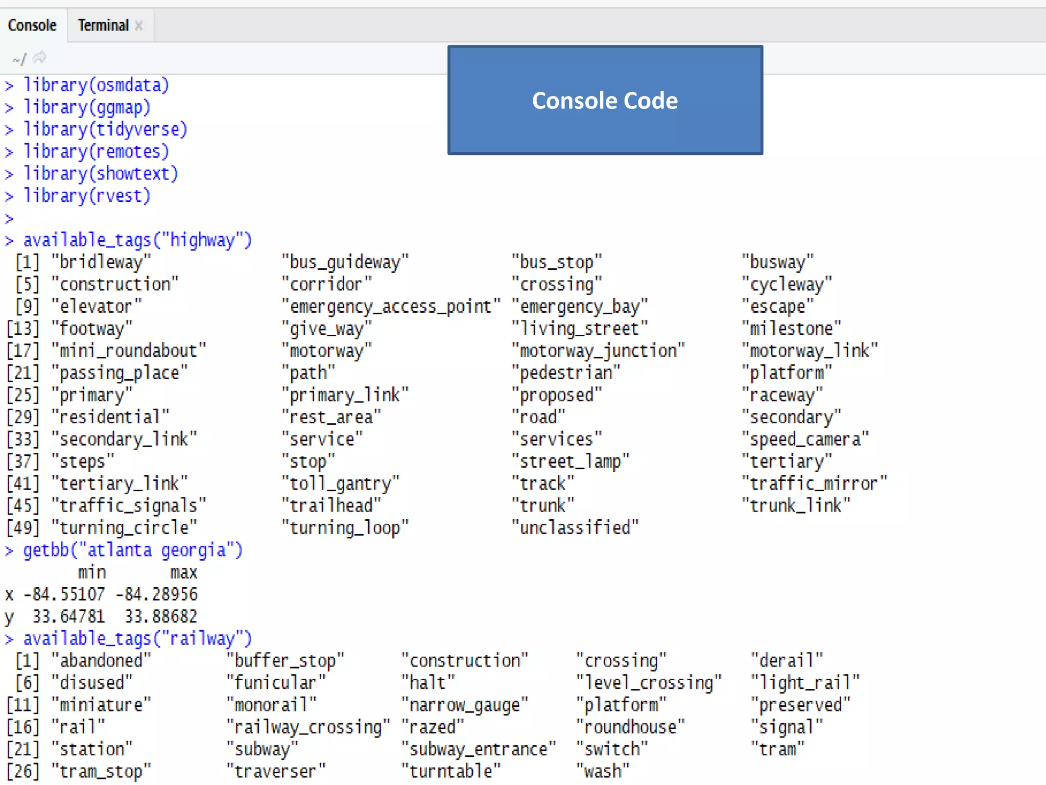
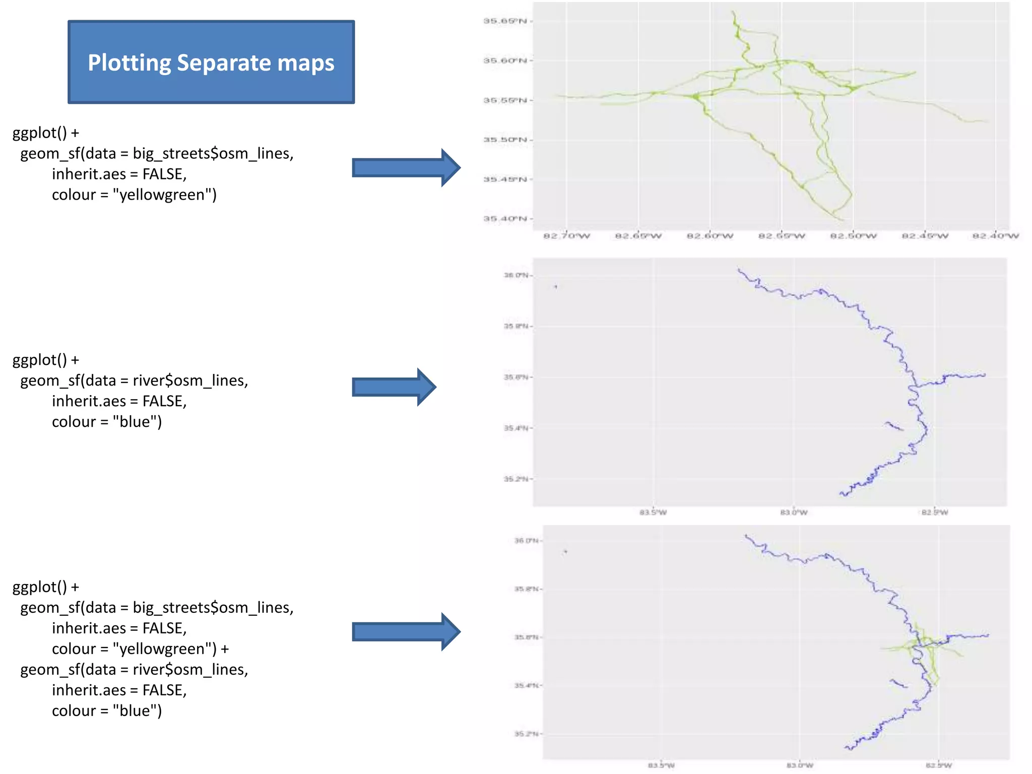
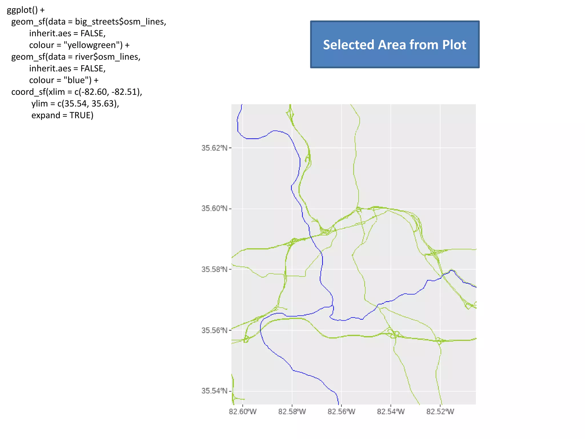
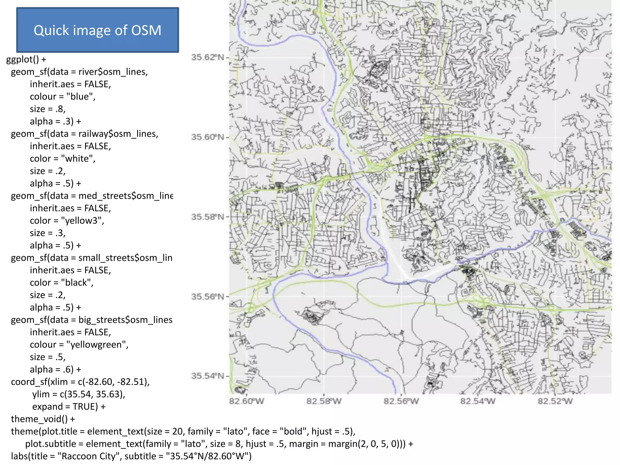
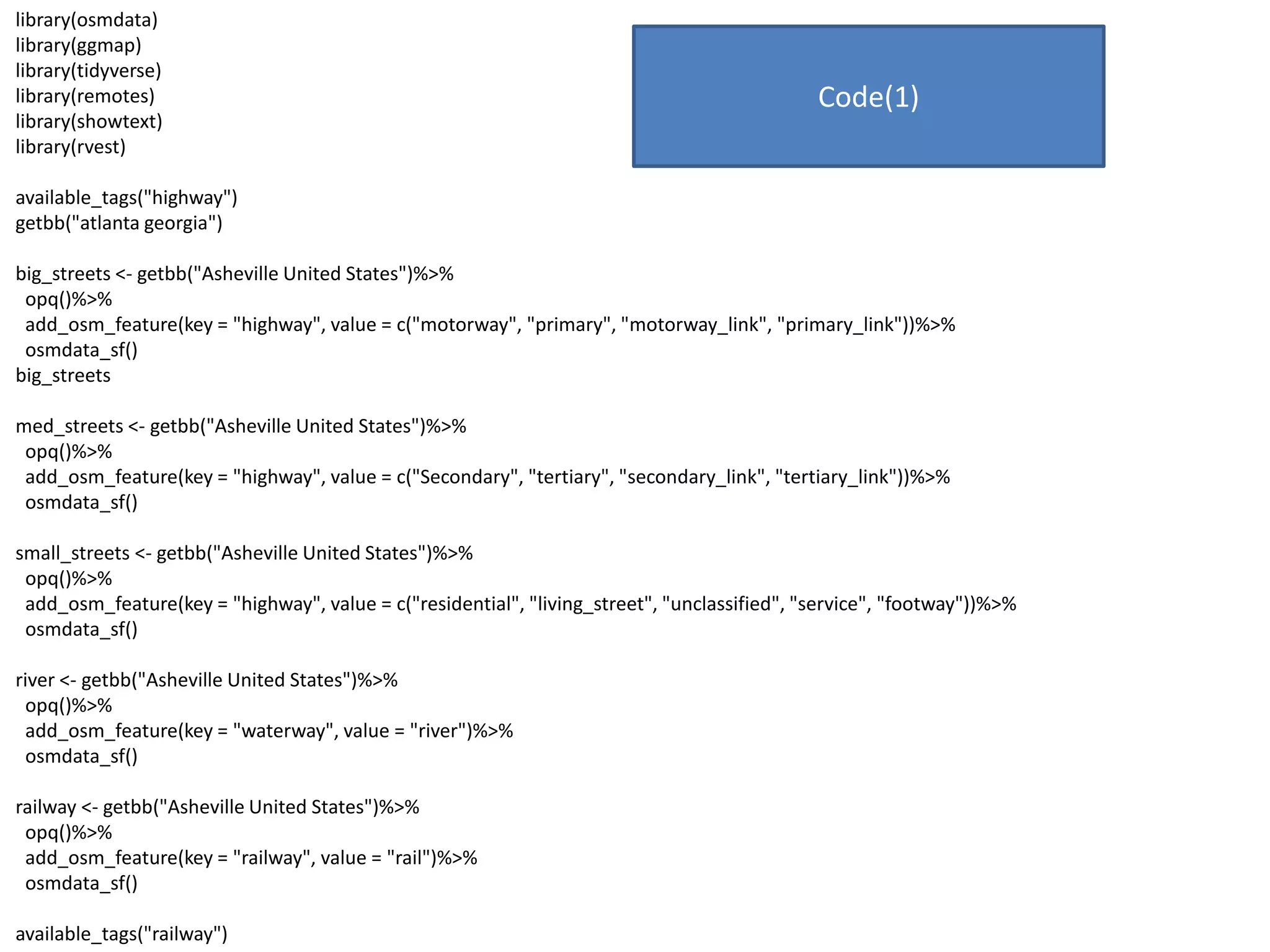
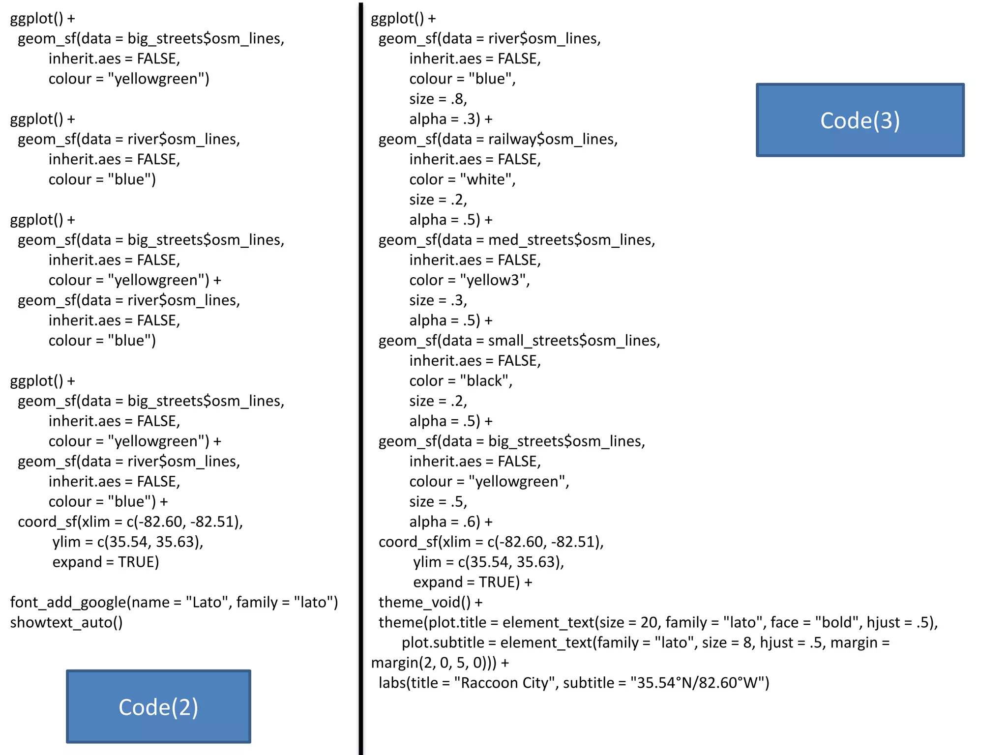
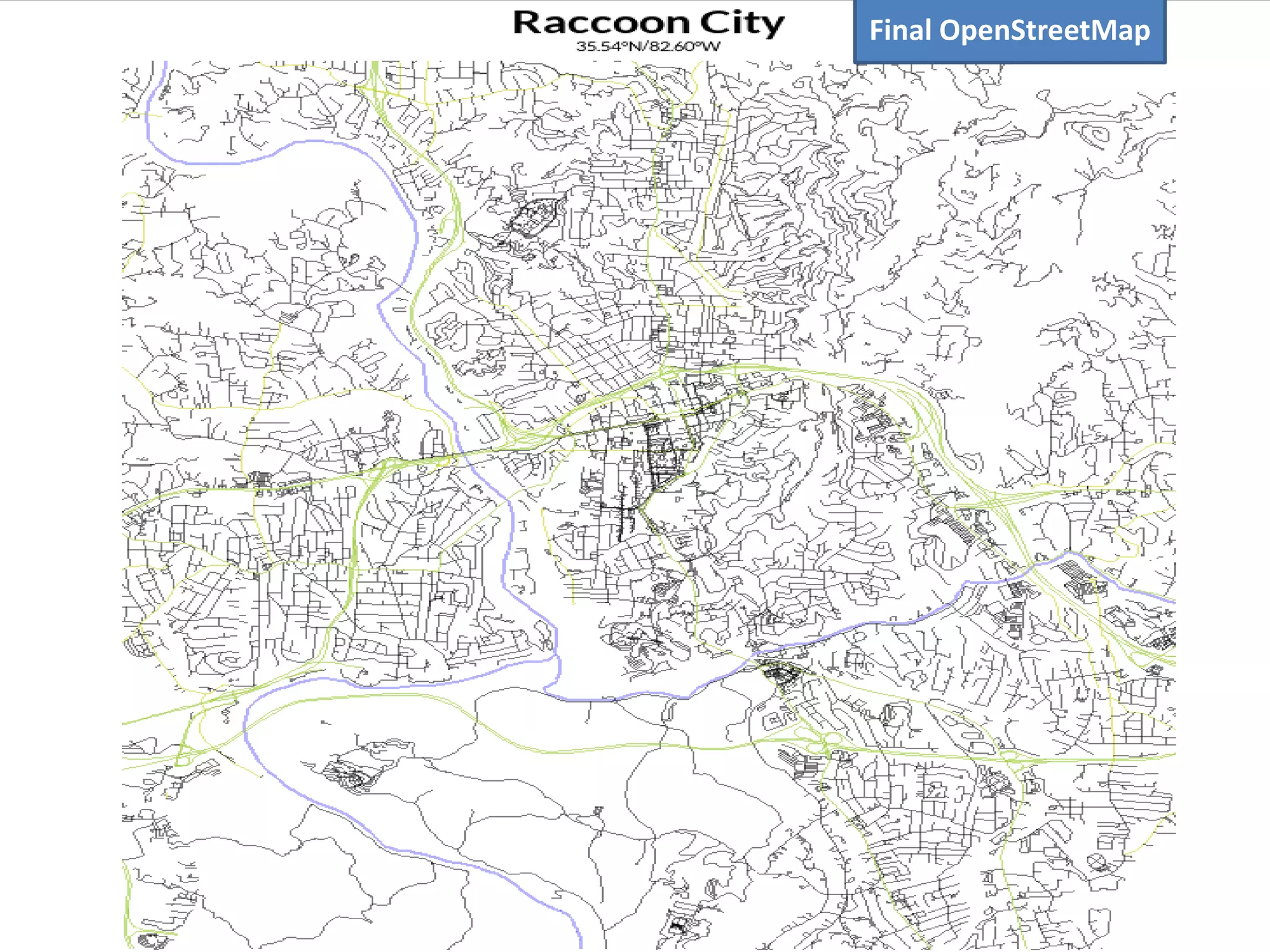
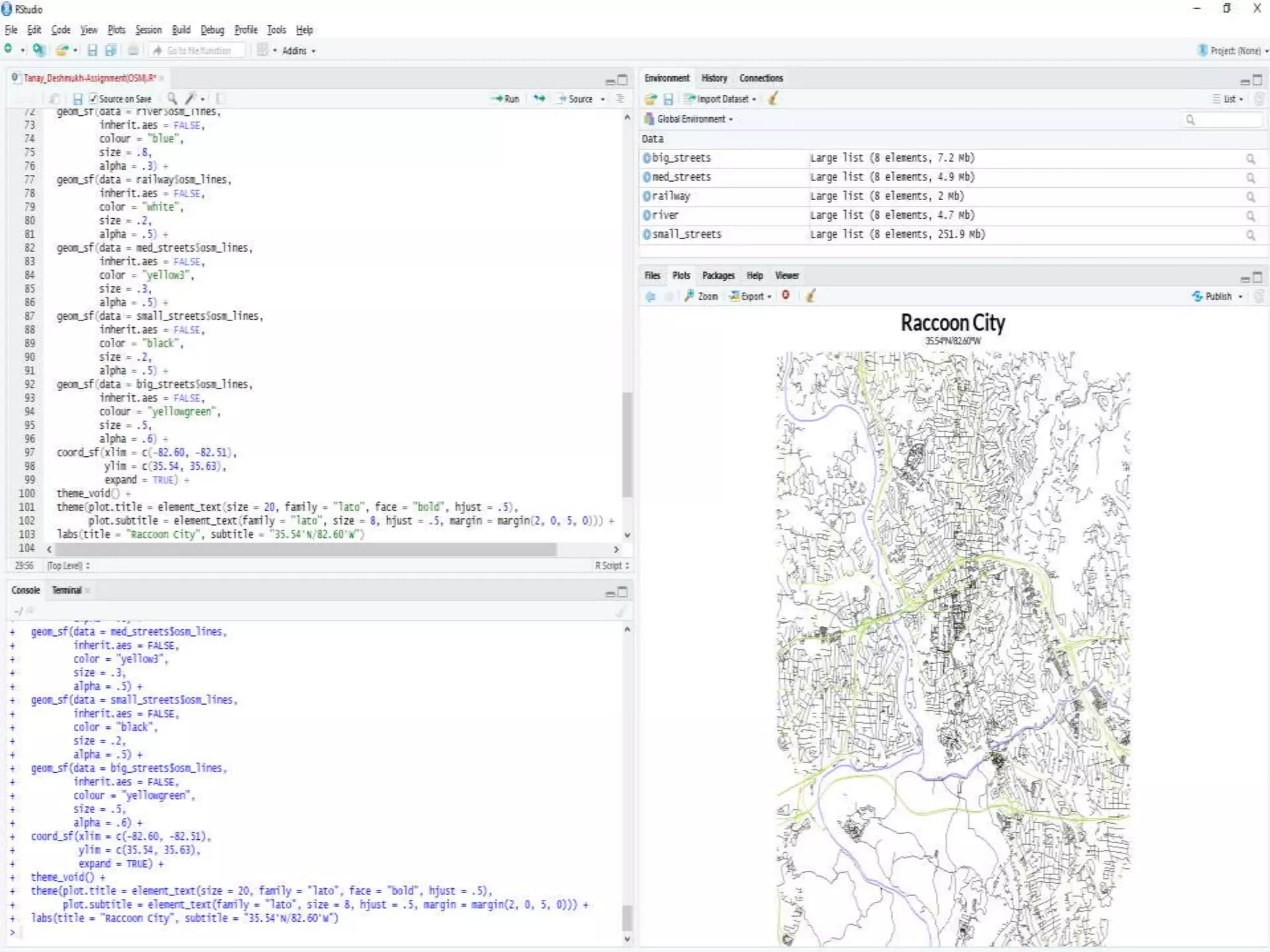
DAVV
School of Data Science and Forecasting
M.sc. (Data Science and Analytics) 2nd Sem
Name - Tanay Deshmukh
Roll Number - DS5B-2034
Subject - Statistical Programming in R
Subject Code - DS5B-508
Assignment Topic - OpenStreetMap(OSM)
Date - 30-06-2021
Submitted to – Mr. Vandit Hedau
Result
Libraries used –
Functions used –
• available_tags()
• getbb()
• add_osm_feature()
• osmdata_sf()
• geom_sf()
• coord_sf()
• etc
Procedure
available_tags("highway")
getbb("atlanta georgia")
big_streets <- getbb("Asheville United States")%>%
opq()%>%
add_osm_feature(key = "highway", value = c("motorway", "primary", "motorway_link", "primary_link"))%>%
osmdata_sf()
big_streets
med_streets <- getbb("Asheville United States")%>%
opq()%>%
add_osm_feature(key = "highway", value = c("Secondary", "tertiary", "secondary_link", "tertiary_link"))%>%
osmdata_sf()
small_streets <- getbb("Asheville United States")%>%
opq()%>%
add_osm_feature(key = "highway", value = c("residential", "living_street", "unclassified", "service", "footway"))%>%
osmdata_sf()
river <- getbb("Asheville United States")%>%
opq()%>%
add_osm_feature(key = "waterway", value = "river")%>%
osmdata_sf()
railway <- getbb("Asheville United States")%>%
opq()%>%
add_osm_feature(key = "railway", value = "rail")%>%
osmdata_sf()
available_tags("railway")
Importing Data
Console Code
ggplot() +
geom_sf(data = big_streets$osm_lines,
inherit.aes = FALSE,
colour = "yellowgreen")
ggplot() +
geom_sf(data = river$osm_lines,
inherit.aes = FALSE,
colour = "blue")
ggplot() +
geom_sf(data = big_streets$osm_lines,
inherit.aes = FALSE,
colour = "yellowgreen") +
geom_sf(data = river$osm_lines,
inherit.aes = FALSE,
colour = "blue")
Plotting Separate maps
ggplot() +
geom_sf(data = big_streets$osm_lines,
inherit.aes = FALSE,
colour = "yellowgreen") +
geom_sf(data = river$osm_lines,
inherit.aes = FALSE,
colour = "blue") +
coord_sf(xlim = c(-82.60, -82.51),
ylim = c(35.54, 35.63),
expand = TRUE)
Selected Area from Plot
ggplot() +
geom_sf(data = river$osm_lines,
inherit.aes = FALSE,
colour = "blue",
size = .8,
alpha = .3) +
geom_sf(data = railway$osm_lines,
inherit.aes = FALSE,
color = "white",
size = .2,
alpha = .5) +
geom_sf(data = med_streets$osm_lines,
inherit.aes = FALSE,
color = "yellow3",
size = .3,
alpha = .5) +
geom_sf(data = small_streets$osm_lines,
inherit.aes = FALSE,
color = "black",
size = .2,
alpha = .5) +
geom_sf(data = big_streets$osm_lines,
inherit.aes = FALSE,
colour = "yellowgreen",
size = .5,
alpha = .6) +
coord_sf(xlim = c(-82.60, -82.51),
ylim = c(35.54, 35.63),
expand = TRUE) +
theme_void() +
theme(plot.title = element_text(size = 20, family = "lato", face = "bold", hjust = .5),
plot.subtitle = element_text(family = "lato", size = 8, hjust = .5, margin = margin(2, 0, 5, 0))) +
labs(title = "Raccoon City", subtitle = "35.54°N/82.60°W")
Quick image of OSM
library(osmdata)
library(ggmap)
library(tidyverse)
library(remotes)
library(showtext)
library(rvest)
available_tags("highway")
getbb("atlanta georgia")
big_streets <- getbb("Asheville United States")%>%
opq()%>%
add_osm_feature(key = "highway", value = c("motorway", "primary", "motorway_link", "primary_link"))%>%
osmdata_sf()
big_streets
med_streets <- getbb("Asheville United States")%>%
opq()%>%
add_osm_feature(key = "highway", value = c("Secondary", "tertiary", "secondary_link", "tertiary_link"))%>%
osmdata_sf()
small_streets <- getbb("Asheville United States")%>%
opq()%>%
add_osm_feature(key = "highway", value = c("residential", "living_street", "unclassified", "service", "footway"))%>%
osmdata_sf()
river <- getbb("Asheville United States")%>%
opq()%>%
add_osm_feature(key = "waterway", value = "river")%>%
osmdata_sf()
railway <- getbb("Asheville United States")%>%
opq()%>%
add_osm_feature(key = "railway", value = "rail")%>%
osmdata_sf()
available_tags("railway")
Code(1)
ggplot() +
geom_sf(data = big_streets$osm_lines,
inherit.aes = FALSE,
colour = "yellowgreen")
ggplot() +
geom_sf(data = river$osm_lines,
inherit.aes = FALSE,
colour = "blue")
ggplot() +
geom_sf(data = big_streets$osm_lines,
inherit.aes = FALSE,
colour = "yellowgreen") +
geom_sf(data = river$osm_lines,
inherit.aes = FALSE,
colour = "blue")
ggplot() +
geom_sf(data = big_streets$osm_lines,
inherit.aes = FALSE,
colour = "yellowgreen") +
geom_sf(data = river$osm_lines,
inherit.aes = FALSE,
colour = "blue") +
coord_sf(xlim = c(-82.60, -82.51),
ylim = c(35.54, 35.63),
expand = TRUE)
font_add_google(name = "Lato", family = "lato")
showtext_auto()
ggplot() +
geom_sf(data = river$osm_lines,
inherit.aes = FALSE,
colour = "blue",
size = .8,
alpha = .3) +
geom_sf(data = railway$osm_lines,
inherit.aes = FALSE,
color = "white",
size = .2,
alpha = .5) +
geom_sf(data = med_streets$osm_lines,
inherit.aes = FALSE,
color = "yellow3",
size = .3,
alpha = .5) +
geom_sf(data = small_streets$osm_lines,
inherit.aes = FALSE,
color = "black",
size = .2,
alpha = .5) +
geom_sf(data = big_streets$osm_lines,
inherit.aes = FALSE,
colour = "yellowgreen",
size = .5,
alpha = .6) +
coord_sf(xlim = c(-82.60, -82.51),
ylim = c(35.54, 35.63),
expand = TRUE) +
theme_void() +
theme(plot.title = element_text(size = 20, family = "lato", face = "bold", hjust = .5),
plot.subtitle = element_text(family = "lato", size = 8, hjust = .5, margin =
margin(2, 0, 5, 0))) +
labs(title = "Raccoon City", subtitle = "35.54°N/82.60°W")
Code(2)
Code(3)
Final OpenStreetMap
Thank You

OpenStreetMap R

  • 1.
    DAVV School of DataScience and Forecasting M.sc. (Data Science and Analytics) 2nd Sem Name - Tanay Deshmukh Roll Number - DS5B-2034 Subject - Statistical Programming in R Subject Code - DS5B-508 Assignment Topic - OpenStreetMap(OSM) Date - 30-06-2021 Submitted to – Mr. Vandit Hedau
  • 2.
  • 3.
    Libraries used – Functionsused – • available_tags() • getbb() • add_osm_feature() • osmdata_sf() • geom_sf() • coord_sf() • etc Procedure
  • 4.
    available_tags("highway") getbb("atlanta georgia") big_streets <-getbb("Asheville United States")%>% opq()%>% add_osm_feature(key = "highway", value = c("motorway", "primary", "motorway_link", "primary_link"))%>% osmdata_sf() big_streets med_streets <- getbb("Asheville United States")%>% opq()%>% add_osm_feature(key = "highway", value = c("Secondary", "tertiary", "secondary_link", "tertiary_link"))%>% osmdata_sf() small_streets <- getbb("Asheville United States")%>% opq()%>% add_osm_feature(key = "highway", value = c("residential", "living_street", "unclassified", "service", "footway"))%>% osmdata_sf() river <- getbb("Asheville United States")%>% opq()%>% add_osm_feature(key = "waterway", value = "river")%>% osmdata_sf() railway <- getbb("Asheville United States")%>% opq()%>% add_osm_feature(key = "railway", value = "rail")%>% osmdata_sf() available_tags("railway") Importing Data
  • 5.
  • 6.
    ggplot() + geom_sf(data =big_streets$osm_lines, inherit.aes = FALSE, colour = "yellowgreen") ggplot() + geom_sf(data = river$osm_lines, inherit.aes = FALSE, colour = "blue") ggplot() + geom_sf(data = big_streets$osm_lines, inherit.aes = FALSE, colour = "yellowgreen") + geom_sf(data = river$osm_lines, inherit.aes = FALSE, colour = "blue") Plotting Separate maps
  • 7.
    ggplot() + geom_sf(data =big_streets$osm_lines, inherit.aes = FALSE, colour = "yellowgreen") + geom_sf(data = river$osm_lines, inherit.aes = FALSE, colour = "blue") + coord_sf(xlim = c(-82.60, -82.51), ylim = c(35.54, 35.63), expand = TRUE) Selected Area from Plot
  • 8.
    ggplot() + geom_sf(data =river$osm_lines, inherit.aes = FALSE, colour = "blue", size = .8, alpha = .3) + geom_sf(data = railway$osm_lines, inherit.aes = FALSE, color = "white", size = .2, alpha = .5) + geom_sf(data = med_streets$osm_lines, inherit.aes = FALSE, color = "yellow3", size = .3, alpha = .5) + geom_sf(data = small_streets$osm_lines, inherit.aes = FALSE, color = "black", size = .2, alpha = .5) + geom_sf(data = big_streets$osm_lines, inherit.aes = FALSE, colour = "yellowgreen", size = .5, alpha = .6) + coord_sf(xlim = c(-82.60, -82.51), ylim = c(35.54, 35.63), expand = TRUE) + theme_void() + theme(plot.title = element_text(size = 20, family = "lato", face = "bold", hjust = .5), plot.subtitle = element_text(family = "lato", size = 8, hjust = .5, margin = margin(2, 0, 5, 0))) + labs(title = "Raccoon City", subtitle = "35.54°N/82.60°W") Quick image of OSM
  • 9.
    library(osmdata) library(ggmap) library(tidyverse) library(remotes) library(showtext) library(rvest) available_tags("highway") getbb("atlanta georgia") big_streets <-getbb("Asheville United States")%>% opq()%>% add_osm_feature(key = "highway", value = c("motorway", "primary", "motorway_link", "primary_link"))%>% osmdata_sf() big_streets med_streets <- getbb("Asheville United States")%>% opq()%>% add_osm_feature(key = "highway", value = c("Secondary", "tertiary", "secondary_link", "tertiary_link"))%>% osmdata_sf() small_streets <- getbb("Asheville United States")%>% opq()%>% add_osm_feature(key = "highway", value = c("residential", "living_street", "unclassified", "service", "footway"))%>% osmdata_sf() river <- getbb("Asheville United States")%>% opq()%>% add_osm_feature(key = "waterway", value = "river")%>% osmdata_sf() railway <- getbb("Asheville United States")%>% opq()%>% add_osm_feature(key = "railway", value = "rail")%>% osmdata_sf() available_tags("railway") Code(1)
  • 10.
    ggplot() + geom_sf(data =big_streets$osm_lines, inherit.aes = FALSE, colour = "yellowgreen") ggplot() + geom_sf(data = river$osm_lines, inherit.aes = FALSE, colour = "blue") ggplot() + geom_sf(data = big_streets$osm_lines, inherit.aes = FALSE, colour = "yellowgreen") + geom_sf(data = river$osm_lines, inherit.aes = FALSE, colour = "blue") ggplot() + geom_sf(data = big_streets$osm_lines, inherit.aes = FALSE, colour = "yellowgreen") + geom_sf(data = river$osm_lines, inherit.aes = FALSE, colour = "blue") + coord_sf(xlim = c(-82.60, -82.51), ylim = c(35.54, 35.63), expand = TRUE) font_add_google(name = "Lato", family = "lato") showtext_auto() ggplot() + geom_sf(data = river$osm_lines, inherit.aes = FALSE, colour = "blue", size = .8, alpha = .3) + geom_sf(data = railway$osm_lines, inherit.aes = FALSE, color = "white", size = .2, alpha = .5) + geom_sf(data = med_streets$osm_lines, inherit.aes = FALSE, color = "yellow3", size = .3, alpha = .5) + geom_sf(data = small_streets$osm_lines, inherit.aes = FALSE, color = "black", size = .2, alpha = .5) + geom_sf(data = big_streets$osm_lines, inherit.aes = FALSE, colour = "yellowgreen", size = .5, alpha = .6) + coord_sf(xlim = c(-82.60, -82.51), ylim = c(35.54, 35.63), expand = TRUE) + theme_void() + theme(plot.title = element_text(size = 20, family = "lato", face = "bold", hjust = .5), plot.subtitle = element_text(family = "lato", size = 8, hjust = .5, margin = margin(2, 0, 5, 0))) + labs(title = "Raccoon City", subtitle = "35.54°N/82.60°W") Code(2) Code(3)
  • 11.
  • 13.