This document is a project report submitted by Omar Omrane to obtain a diploma in engineering from the National School of Engineering of Monastir in Tunisia. The report is focused on artificial lift design and simulation using AutographPC software. It includes dedications to his family for their support and acknowledgments to his academic and industrial supervisors for their guidance. It also provides lists of figures and tables and introduces the general topics that will be discussed in each chapter, including an overview of the oil and gas industry, electrical submersible pumps, and a case study on pump sizing.

1. Ministère de l’Enseignement Supérieur et de la Recherche Scientifique
*-*-*-*-*-*-*-*
Université de Monastir
*-*-*-*-*-*-*-*
Ecole Nationale d’Ingénieurs de Monastir
*-*-*-*-*-*-*-*
Année Universitaire : 2015/2016
MEMOIRE
DE
PROJET DE FIN D’ETUDES
PRESENTE POUR OBTENIR LE
DIPLÔME NATIONAL
D’INGENIEUR
Spécialité : GENIE ENERGETIQUE
Par
Omar OMRANE
Né le : 06/07/1992 à Sfax
Artificial lift design:
ESP design and simulation with AutographPC Software
Soutenu le 02/06/2016 ; devant le jury d’examen:
Hacen DHAHRI Président
Med Naceur BORGINI Membre
Walid HASSEN Encadrant académique
Med Ali KHYARI Encadrant industriel

2. Dedication
This project owes its existence to a number of people to whom I feel genuinely
obliged
To my dear mother Nassima, my greatest teacher, a teacher of love, compassion
and bravery, you will always be the biggest inspiration in my life.
May God give you long life full of joy and happiness.
To my dear father Jamel, to whom I owe the best of myself, my teacher of love.
This project could not be realized without your belief in me, your encouragement,
your trust, your moral and material support.
May God give you long life full of joy and happiness.
To my beloved brothers; Ahmed and Zied, for always being there by my side,
for the confidence you provide me and for your encouragement.
Finally I thank everyone who in one way or another helped me achieving this
work.
I dedicated this work
Omar Omrane

3. Acknowledgment
This project would not have the spirit that it has without the supervision of
my academic supervisor Mr. Walid HASSEN, Assistant Professor at national
school of engineering of Monastir and my industrial supervisor Mr. Mohamed
Ali KHIYARI, Production engineer at OMV Tunisia. I would like to express
my sincere appreciation of their constant willingness to share their immense
knowledge and experience during this four months period. Their valuable
guidance and support helped in accomplishing this project.
I express my gratitude toward OMV exploration and production staff for
giving me the opportunity to integrate the professional life through this
internship and affording a warm welcome environment during my training
within their company.
I will forever remember, Mrs. Yesmine LAROUSSI and Mr. Brahim
LETAIEF for inspiring positive energy and healthy work environment.
We must not forget the contribution of my beloved friends; Salma
LATRACH, Khaled MNEJJA and Mohamed CHEMAKH for sharing with me
the funniest moments and the lovely experience that we lived during this
internship.
Last and not least, I wish to express my sense of gratitude to all who directly
or indirectly have laid their hand in this venture

4. Summary
List of figures
List of tables
General Introduction................................................................................................................................ 1
Company presentation............................................................................................................................. 2
General description.............................................................................................................................. 3
Objective ............................................................................................................................................. 3
Field of activity ................................................................................................................................... 3
Chapter I: Oil and Gas general overview .................................................................................... 4
I.1. Introduction....................................................................................................................................... 5
I.2. Presentation of the petroleum production system ............................................................................. 6
I.2.1. Definition ................................................................................................................................... 6
I.2.2. Pressure losses across the petroleum production system ........................................................... 6
I.3. Petroleum production engineering................................................................................................... 7
I.3.1. Introduction............................................................................................................................... 7
I.3.2. Production optimization and well performance ......................................................................... 7
I.3.2.1. Well performance: Nodal system analysis.......................................................................... 7
I.3.2.2. Artificial lift ...................................................................................................................... 12
I.4. Properties of reservoir fluids and phase behavior........................................................................... 15
I.4.1. Multiphase flow theory patterns and map.................................................................................... 15
I.4.2. Bubble point............................................................................................................................. 17
I.4.3. GOR (Gas Oil Ratio)................................................................................................................ 17
I.4.4. FVF(Formation Volume Factor).............................................................................................. 17
I.4.4.1. Formation Volume Factor (oil) ......................................................................................... 17
I.4.4.2. Formation Volume Factor (gas)........................................................................................ 17
I.4.5. Water cut (WC)........................................................................................................................ 18
I.4.6. Oil density................................................................................................................................ 18
I.5. Conclusion ...................................................................................................................................... 19
Chapter II: Electrical Submersible Pump(ESP) ...................................................................... 20
II.1. Introduction.................................................................................................................................... 21
II.1.1. General history of ESP ........................................................................................................... 21
II.1.2. General overview of ESP........................................................................................................ 21
II.2. ESP components............................................................................................................................ 22
II.2.1. ESP down-hole components................................................................................................... 23
II.2.1.1 Pump................................................................................................................................ 23

5. II.2.1.2 Gas separator ................................................................................................................... 24
II.2.1.3. Seal section...................................................................................................................... 25
II.2.1.4. Electrical motor................................................................................................................ 26
II.2.2. ESP Surface components........................................................................................................ 26
II.2.2.1. Junction Box.................................................................................................................... 26
II.2.2.2 Power cable....................................................................................................................... 27
II.2.2.3. Motor controller............................................................................................................... 27
II.2.2.4. ESP variable speed drive ................................................................................................. 27
II.2.2.5. Transformer ..................................................................................................................... 27
II.2.3. ESP mainly support equipment............................................................................................... 27
II.3. Performance of an ESP system...................................................................................................... 28
II.4. Evaluation of ESP components...................................................................................................... 29
II.4.1 ESP advantages........................................................................................................................ 29
II.4.2. ESP disadvantages.................................................................................................................. 29
II.5. Conclusion..................................................................................................................................... 30
Chapter III: Case study................................................................................................................... 31
III.1. Hand sizing................................................................................................................................... 32
III.1.1. The 9 steps procedure............................................................................................................ 32
III.1.1.1 Basic data ....................................................................................................................... 34
III.1.1.2. Production capacity ........................................................................................................ 36
III.1.1.3. Gas calculation ............................................................................................................... 39
III.1.1.4. Total dynamic head ........................................................................................................ 43
III.1.1.5. Pump selection................................................................................................................ 45
III.1.1.6. Seal section selection...................................................................................................... 50
III.1.1.7 Motor selection................................................................................................................ 51
III.1.1.8. Power cable selection ..................................................................................................... 53
III.1.1.9. Motor controller selection .............................................................................................. 56
III.2. Software design............................................................................................................................ 60
III.2.1. AutographPC brief overview................................................................................................. 60
III.2.2. AutographPC purpose ........................................................................................................... 61
III.2.3. AutographPC features ........................................................................................................... 61
III.2.4. AutographPC modeling Application (Cherouq 1 well)......................................................... 61
III.2.4.1. Problematic and Purpose ................................................................................................ 61
III.2.4.2. Data required for design................................................................................................. 61
III.2.4.3. Pump sizing screen......................................................................................................... 64
III.2.4.4. Motor sizing screen ........................................................................................................ 65

6. III.2.4.5. Seal sizing screen ........................................................................................................... 66
III.2.4.6. Cable sizing screen......................................................................................................... 66
III.2.4.7. Controller sizing screen.................................................................................................. 67
III.3. Conclusion.................................................................................................................................... 68
Chapter IV: Economic Study........................................................................................................ 69
IV.1. Project net cashflow .................................................................................................................... 70
IV.2. Excel results ................................................................................................................................ 71
IV.3. Interpretation................................................................................................................................ 74
IV.4. Conclusion.................................................................................................................................... 75
General conclusion................................................................................................................................ 76
References .

7. List of figures
Chapter I
Figure I- 1: Petroleum Production System.............................................................................................. 6
Figure I- 2: main pressure losses within production system ................................................................... 7
Figure I- 3: Straight-line IPR (for an incompressible liquid).................................................................. 9
Figure I- 4: Vogel 's inflow performance curve .................................................................................... 10
Figure I- 5: Inflow Performance Relationship....................................................................................... 10
Figure I- 6: TPR curves for different wellhead pressures ..................................................................... 11
Figure I- 7: Operating point................................................................................................................... 12
Figure I- 8: Typical rod pump ............................................................................................................... 13
Figure I- 9: Hydraulic pump.................................................................................................................. 13
Figure I- 10: ESP system....................................................................................................................... 14
Figure I- 11: Gas lift system.................................................................................................................. 14
Figure I- 12: Vertical flow patterns....................................................................................................... 16
Figure I- 13: Horizontal flow patterns................................................................................................... 16
Chapter II
Figure II- 1: Conventional ESP installation .......................................................................................... 22
Figure II- 2: ESP submersible pump cutaway....................................................................................... 23
Figure II- 3: Illustration of impeller and subcomponents...................................................................... 23
Figure II- 4: illustration cutaway of a diffuser ...................................................................................... 24
Figure II- 5: Illustration of a pump stage............................................................................................... 24
Figure II- 6: Pump intake ...................................................................................................................... 24
Figure II- 7: Rotary gas separator.......................................................................................................... 25
Figure II- 8: ESP combined seal section components........................................................................... 26
Figure II- 9: ESP motor cutaway illustration ........................................................................................ 26
Figure II- 10: example performance curve of an ESP pump................................................................. 28
Chapter III
Figure III- 1: Total dynamic head ......................................................................................................... 44
Figure III- 2: Pump performance curve 538 series P37 Centurion pump.............................................. 48
Figure III- 3: Pump performance curve 538 series P23 Centurion pump.............................................. 48
Figure III- 4: Pump performance curve 538 series G31 Centurion pump............................................. 49
Figure III- 5: Horsepower VS Total dynamic head in feet.................................................................... 51
Figure III- 6: well conditions screen capture......................................................................................... 62
Figure III- 7: Pump sizing screen capture ............................................................................................. 64
Figure III- 8: Motor sizing screen capture............................................................................................. 65
Figure III- 9: Seal sizing screen capture................................................................................................ 66
Figure III- 10: Cable sizing screen capture ........................................................................................... 66
Figure III- 11: controller sizing screen capture .................................................................................... 67
Chapter IV
Figure IV- 1: Production decline profile ............................................................................................... 74
Figure IV- 2: Cashflow profile.............................................................................................................. 74

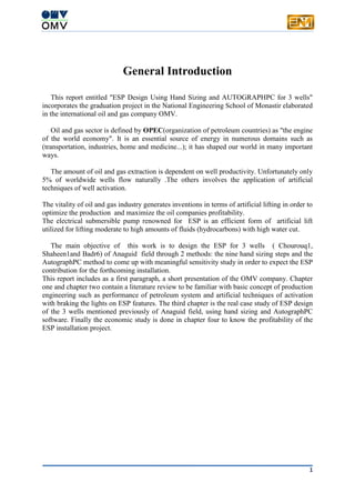
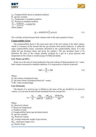
8. List of tables
Chapter I
Table I- 1: Advantages and Disadvantages of artificial lift technologies[4]......................................... 15
Chapter III
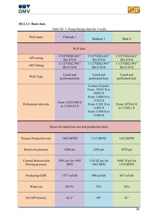
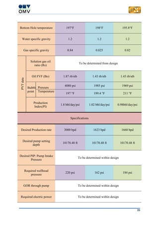
Table III- 1: Pump Design data for 3 wells ........................................................................................... 34
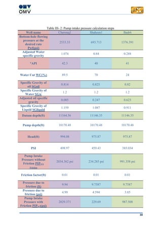
Table III- 2: Pump intake pressure calculation steps............................................................................. 38
Table III- 3: Free gas calculation steps.................................................................................................. 41
Table III- 4: Total Dynamic head calculation ....................................................................................... 45
Table III- 5: Required Data for pump selection .................................................................................... 46
Table III- 6: Pump specifications .......................................................................................................... 49
Table III- 7: Seal horsepower estimation .............................................................................................. 51
Table III- 8: required motor power........................................................................................................ 52
Table III- 9: motor selection specification ............................................................................................ 52
Table III- 10: Motor load calculation.................................................................................................... 52
Table III- 11: Line losses per 1000 ft calculation.................................................................................. 53
Table III- 12: Temperature correction factor estimation....................................................................... 53
Table III- 13: Voltage drop per 1000 ft calculation............................................................................... 54
Table III- 14: Total voltage drop calculation ........................................................................................ 54
Table III- 15: Motor nameplate voltage drop calculation...................................................................... 55
Table III- 16: Power cable's operating temperature. ............................................................................. 55
Table III- 17: Surface Voltage calculation ............................................................................................ 56
Table III- 18: Motor controller specifications....................................................................................... 57
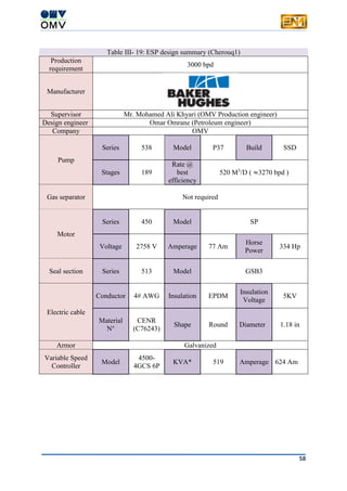
Table III- 19: ESP design summary (Cherouq1)................................................................................... 58
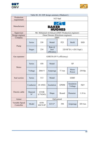
Table III- 20: ESP design summary (Shaheen1) ................................................................................... 59
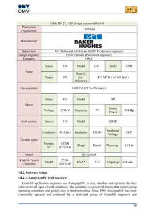
Table III- 21: ESP design summary(Badr6).......................................................................................... 60
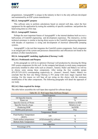
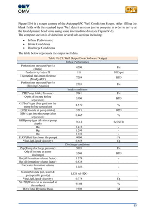
Table III- 22: Well input Data (Software Design)................................................................................. 61
Table III- 23: Well Output Data (Software Design).............................................................................. 63
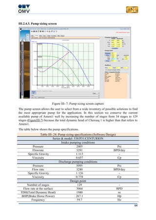
Table III- 24: Pump sizing specifications (Software Design) ............................................................... 64
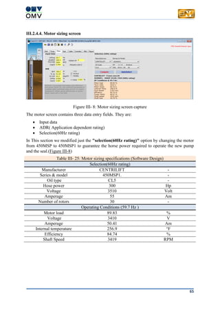
Table III- 25: Motor sizing specifications (Software Design)............................................................... 65
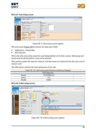
Table III- 26: Seal sizing specifications (Software Design).................................................................. 66
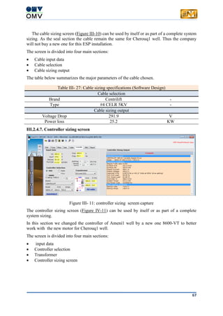
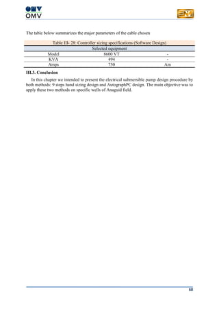
Table III- 27: Cable sizing specifications (Software Design) ............................................................... 67
Table III- 28: Controller sizing specifications (Software Design) ........................................................ 68
Chapter IV
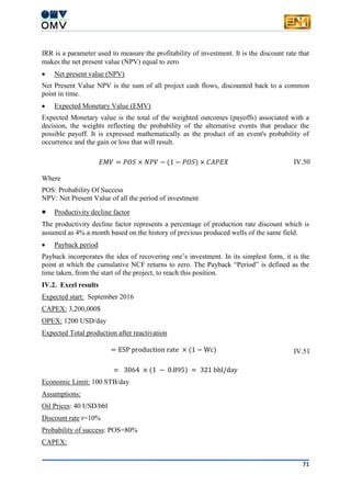
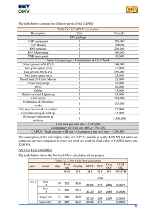
Table IV- 1: CAPEX calculation........................................................................................................... 72
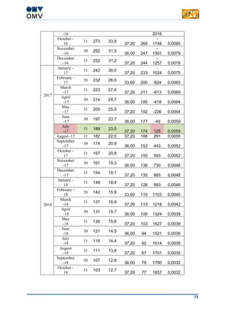
Table IV- 2: Net Cash Flow calculation................................................................................................ 72

9. Glossary of terms and acronyms
A
API: American Petroleum Institute
AOF: Absolute Oil Flowrate
AWSG: Adjusted Water Specific Gravity
AOSG: Adjusted Oil Specific Gravity
B
BEP: Best Efficiency Point
BHP: Brake Horse Power
BBL: Barrel (42 US Gallons)
BFPD: Barrel of Fluid Per Day
BPD: Barrel Per Day
Bg: gas formation volume factor
Bo: Oil Formation volume Factor
BOPD: Barrel of Oil Per Day
BHT: Bottom-Hole Temperature
C
cP: centripoise
D
DWHP: Desired Wellhead Pressure
E
ESP: Electric submerged pump
F
FVF: Formation Volume Factor
Ft: feet
FL: Friction Loss
Fg: Volume of free gas
G
GOR: Gas Oil Ratio
H
HP: High pressure
HP: Horse Power
I
IPR : Inflow Performance Relationship
ID: Inside Diameter
M
Mg: average molecular weight of gas mixture
Mair: molecular weight of air
𝑚 𝑔: mass of gas
mcf: a traditional unit of volume equal to
1000 cubic foot
N
NPSH: Net Positive Suction Head
n: Number of mole
O
OD: Outside Diameter
P
PR: reservoir pressure
Pwf: flowing bottom-hole pressure
PI: Productivity Index
Psc: Pressure in standard condition
PSI: Pound per Square Inch
Psia: pound per square inch, absolute
Psig: pound per square inch, gauge
PIP: Pump Intake Pressure
Pb: bubble point pressure
PSD: Pump Setting Depth
Pd: discharge pressure (well head pressure)
Q
Q: Flowrate
Qd: desired flowrate
R
RPM: Rotation Per Minute
rcf : cubic feet of reservoir volume
R: gas-law constant
rb: barrel at reservoir conditions
Rs: Solution gas Oil Ratio
S
STB: Stock Tank Barrel
scf : standard cubic foot
SGw: Specific Gravity of Water
SGoil: Specific Gravity of oil
SGliquid: Specific Gravity of liquid
SGgas: Specifig Gravity of gas.
T
TPR: Tubing Performance Relationship
TR: Reservoir Temperature
Tsc: Temperature T standard condition
Tg: total volume of gas at the surface
TDH: Total Dynamic Head
V
VSD: Variable speed drives
VLP: Vertical Lift Performance
VR: Reservoir volume
Vsc: Volume at standard condition
W
Wc: Water Cut
𝜌 𝑔: density of gas
𝛾𝑔: Specific gravity of gas
𝜇0: average viscosity

10. 1
General Introduction
This report entitled "ESP Design Using Hand Sizing and AUTOGRAPHPC for 3 wells"
incorporates the graduation project in the National Engineering School of Monastir elaborated
in the international oil and gas company OMV.
Oil and gas sector is defined by OPEC(organization of petroleum countries) as "the engine
of the world economy". It is an essential source of energy in numerous domains such as
(transportation, industries, home and medicine...); it has shaped our world in many important
ways.
The amount of oil and gas extraction is dependent on well productivity. Unfortunately only
5% of worldwide wells flow naturally .The others involves the application of artificial
techniques of well activation.
The vitality of oil and gas industry generates inventions in terms of artificial lifting in order to
optimize the production and maximize the oil companies profitability.
The electrical submersible pump renowned for ESP is an efficient form of artificial lift
utilized for lifting moderate to high amounts of fluids (hydrocarbons) with high water cut.
The main objective of this work is to design the ESP for 3 wells ( Chourouq1,
Shaheen1and Badr6) of Anaguid field through 2 methods: the nine hand sizing steps and the
AutographPC method to come up with meaningful sensitivity study in order to expect the ESP
contribution for the forthcoming installation.
This report includes as a first paragraph, a short presentation of the OMV company. Chapter
one and chapter two contain a literature review to be familiar with basic concept of production
engineering such as performance of petroleum system and artificial techniques of activation
with braking the lights on ESP features. The third chapter is the real case study of ESP design
of the 3 wells mentioned previously of Anaguid field, using hand sizing and AutographPC
software. Finally the economic study is done in chapter four to know the profitability of the
ESP installation project.

11. 2
Company presentation

12. 3
General description
OMV is a German abbreviation ("österreichische mineralölverwaltung") which means
Austrian mineral oil administration. OMV is an integrated international oil and gas company,
headquartered in Vienna. OMV's main business is in Exploration & Production (E&P), Gas &
Power (G&P) and Refining & Marketing (R&M). With group sales of more than € 42.41
billion and a global workforce of around 26,800 in 2016, OMV is the largest listed
manufacturing company in Austria.
Objective
The main objectives of OMV are:
 Manage exploration and production of hydrocarbon on behalf of the Tunisian
government.
 Producing oil that will allow Tunisia to accelerate its economic development and
establish position on the world stage.
Field of activity
 Exploration and production of hydrocarbon
 Marketing of crude oil and petroleum products
 oil Service
 Human Resources Development

13. 4
Chapter I: Oil and Gas general overview
Objective
The main purpose of this chapter is to
be familiar with the concept of oil and
gas highlighting a major section of
this sector which is production
activity.

14. 5
I.1. Introduction
Petroleum production engineering is the series of activities concerned with the ability of a
well to produce. These activities are divided, according to their specification, into upstream
sector and downstream sector:
 The upstream sector, it mainly consists in searching and finding oil from underground
(underwater) fields called "Exploration" followed by oil or gas extraction "Production".
EXPLORATION
Reservoir capacity is determined approximately by two different methods:
 Geological survey: In this case geoscientists attempt to locate best areas by examining
different underground layers of rock using advanced technologies and special tools such as
"aerial photography, satellite pictures and specialized machines that measure variation in the
earth's gravity fields."
 Seism survey is a vital part in oil and gas exploration, it involves using sound waves
to form a clear picture of underwater layer rock. Surveyors register the seismic waves that are
produced by an explosion or sound generator. This technique is based on determinations of
the time interval that elapses between the initiation of a seismic wave at a selected shop point
and the arrival of reflected or refracted impulses at one or more seismic detectors.
After designating the specific area based on geoscientists investigation the second step should
be begin which is the initial drilling. If drilled wells, called wildcat well, present good signs
of existing crude oil inside then the well will be completed and the second phase of
production starts.
PRODUCTION
Once oil is found after the preliminary exploration phase and the drilling of exploratory
wells, the production phase can begin: wells are perforated adopting the rotary rig drilling's
technique. During this operation underground water should be protected from oil and gas
contamination, thus outer casings must be inserted in the well then cemented to the exterior
wall. Once the reservoir rock is reached the well is completed with the remaining facilities:
wellhead and surface equipments.
 The downstream sector: The downstream sector is the part of the oil industry involved
with purifying crude oil and refining it into different products. It also involves the
transportation and marketing of crude oil and its products.
Once oil starts flowing, it needs to be extracted in large volumes and then taken to special
sites where it is treated carefully before being transported internationally.
The process through which crude oil is purified and treated to remove unusable substances is
called Refining. This process is also used to separate oil into different usable petroleum
products. All this takes place in an oil refinery. Refineries are highly automated and
technologically advanced. That is why a typical refinery costs billions of dollars to build. It
also costs millions to operate, employing hundreds of people and running every day of the
year. All refineries perform three basic functions: Separation, Conversion and Treatment.
Separation
In this phase, a refinery heats crude oil to different temperature levels. Different parts of
crude oil have different boiling points. As the temperature rises, these different parts or
fractions are separated. This is done inside distillation towers.
Conversion
In this phase, high temperatures and pressure, as well as chemical catalysts, are used to
‘crack’ or split heavy hydrocarbon molecules into smaller, more desirable ones. This is the
most widely used conversion method and it is called CRACKING.

15. 6
Treatment
The final phase is treatment. In this step, the fractions produced during separation are
treated to improve their quality. They are then blended with other elements to produce the
final products.
I.2. Presentation of the petroleum production system
I.2.1. Definition
Petroleum production involves two distinct but intimately connected general systems: the
reservoir, which is a porous medium with unique storage and flow characteristics; and the
artificial structures, which include the well, bottom hole, and wellhead assemblies, as well as
the surface gathering, separation, and storage facilities as shown in Figure I-1.
Figure I- 1: Petroleum Production System
I.2.2. Pressure losses across the petroleum production system
The hydrocarbon fluid streams from the reservoir into the well, up the tubing, along the
horizontal flow line and into the oil storage tank. During this process the fluid’s pressure is
reduced from the reservoir pressure to atmosphere pressure in a series of pressure loss
processes (Figure I.2)
These pressure losses can be classified into four main components:
 the total pressure losses in the reservoir
 the total pressure losses in the completion
 the total pressure losses in the tubing
 the total pressure losses at the surface

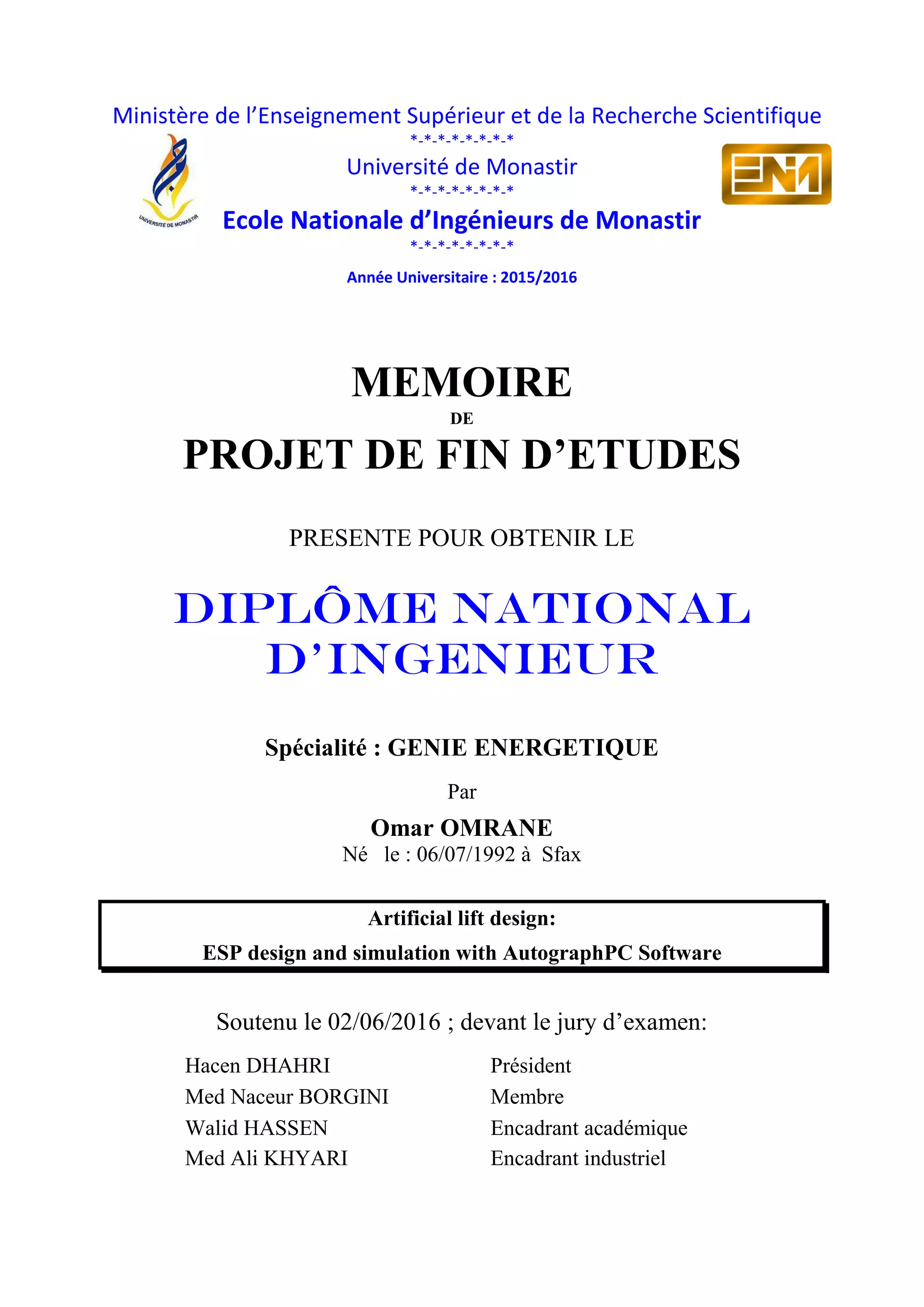
16. 7
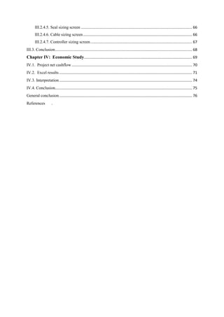
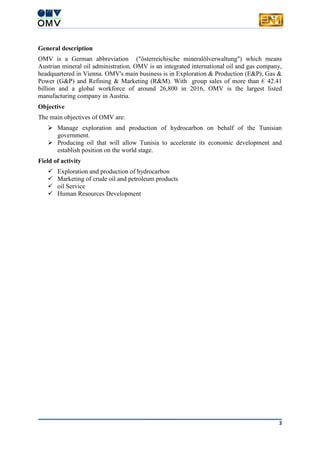
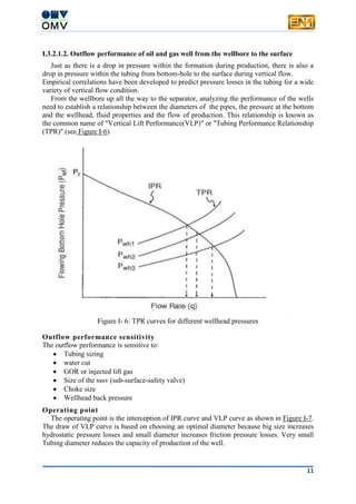
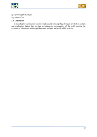
Figure I- 2: main pressure losses within production system[1]
I.3. Petroleum production engineering
I.3.1. Introduction
Production engineering technologies attempt to maximize oil and gas production in a most
possible profitable way. It offers different methods and technologies allowing to:
 Evaluate inflow and outflow performance between the reservoir and the wellbore.
 design completion system
 Select the proper artificial lift equipment
 Select equipment for surface facilities
The only way to achieving these previous responsibilities, is for production engineers to
elaborate a detailed analysis of these distinct, yet related parts:
o The components of oil and gas production system
o The fundamentals of well performance
o well completion
o oil wells activation systems
I.3.2. Production optimization and well performance
I.3.2.1. Well performance: Nodal system analysis
Well analysis is the most important step to optimize oil production. Production
optimization aims to find the flow rate of the producing well based on various approaches.
Over the years oil and gas industry have been resorted to a numerous optimization tools and
techniques to support decisions in order to reach the highest production performance possible.
One of these techniques is designing production systems and facilities.
This depends upon 'NODAL' system analysis approach. It involves employing correlations
to predict multiphase flow behavior through pipes, well completions, restrictions and the
reservoir. For this reason experts specialized in production optimization employ tow methods:
Well inflow performance relationship (IPR) and tubing performance relationship.

17. 8
I.3.2.1.1. Inflow performance from the reservoir to the wellbore
The relationship between bottom-hole pressure and corresponding production rates is of a
paramount importance for the description of well behavior. this is called the well's inflow
performance relationship (IPR) and usually obtained by running well tests.
Productivity Index concept
The productivity index is a mathematical measure of the well potential or ability to produce
and is a commonly measured well property. It's the most optimistic approach to describe the
inflow performance of oilfield wells.
To utilize this concept, four assumptions have to be realized:
 Radial flow near the wellbore area
 A single phase, incompressible liquid is flowing
 A homogeneous distribution of the formation permeability
 The fluid is fully saturated in the formation
For general flow through porous media:
𝑄 =
𝐾𝐴(𝑃0 − 𝑃1)
𝜇𝐿
I.1
But in our case we're working with oil reservoirs to find the production rate of any oil well or
the Darcy law equation:[2]
𝑄 =
7.08. 10−3
ℎ𝐾0(𝑃𝑟 − 𝑃 𝑤𝑓)
𝐵0 𝜇0 ln((
𝑟𝑒
𝑟𝑤
) − 0.75)
I.2
where
𝐵0: liquid volume factor, bbl/STB
𝜇0: average viscosity, cP
𝑟𝑒: drainage radius of well, ft
𝑟𝑤: radius of wellbore, ft
𝐾0: effective permeability, md
ℎ: effective feet of pay(height), ft
𝑃𝑟: reservoir pressure, psi
𝑃 𝑤𝑓: flowing bottom-hole pressure, psi
If we make the assumption that ℎ, 𝐾0, 𝑟𝑤, 𝑟𝑒, 𝜇0 𝑎𝑛𝑑 𝐵0 are constant for a particular well the
equation becomes:
𝑞 = 𝐾(𝑃𝑅 − 𝑃 𝑤𝑓) I.3
where K is the Productivity Index.
Finally we obtain the equation I.4.
𝑞 = 𝑃𝐼(𝑃𝑅 − 𝑃 𝑤𝑓) I.4
PI is usually found by measurement (down-hole gauge and surface flow rate).
It calculates the highest maximum flow rate (AOF) since no change from producing below
bubble point is assumed.

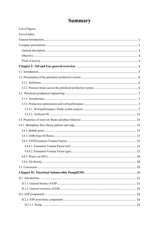
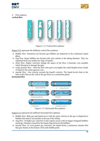
18. 9
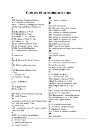
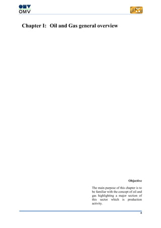
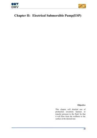
Figure I- 3: Straight-line IPR (for an incompressible liquid) [1]
We can notice in Figure I.3 that the curve of the wellbore flowing pressure (Pwf) in
function of the flow rate (q) is a straight line of a negative slope (−1/PI). Also this graph
shows two important points : The first one ,located on the x-axis, represents the maximum of
the potential rate corresponding to the minimum of the wellbore flowing pressure which is
zero whereas the second one ,located on the y-axis matches the two values of the minimum
flow rate (zero) and the maximum wellbore pressure (Pr: reservoir pressure) that can be
attained.
the maximum flow rate which is impossible to achieve is called typically Absolute Open
Flow Potential typically known for the abbreviation AOF. This latter is used only to compare
between different wells' deliverability. So to obtain the flow rate at any flowing bottom-hole
pressure it's sufficient to know the productivity index PI, the bottom-hole pressure Pwf and
apply the equation I.4. the productivity index is defined as the flow rate per unit pressure
drop.
Voglel's method
When two phase inflow is taking place in the well, straight line IPR are not applicable.
After a thorough study concerned inflow performance relationship of the well with a solution
gas Vogel proposed the following equation.[2]
𝑄
𝑄 𝑚𝑎𝑥
= 1 − 0.2 (
𝑃 𝑤𝑓
𝑃𝑅
) − 0.8 (
𝑃 𝑤𝑓
𝑃𝑅
)
2
I.5
where
Q: liquid rate, STB/day
Qmax: maximum rate at bottom-hole pressure (Pwf), STB/day
PR: average reservoir pressure, psi
Pwf: bottom-hole flowing pressure, psi
Figure I.4 represents Vogel's inflow performance curve.

19. 10
Figure I- 4: Vogel 's inflow performance curve
Sum up IPR
When multi-rate test data is available the straight line IPR and the Vogel IPR curve are
combined to create a new one describing the well performance when the reservoir pressure is
above the bubble point while the wellbore pressure is below. The resulting straight line has a
slope of (1/𝑛). Figure I-5 compares the production rate as a function of drawdown for an
under-saturated oil (straight line IPR, line A) and a saturated oil showing the two phase flow
effects discussed above (curve B).
Figure I- 5: Inflow Performance Relationship[2]

20. 11
I.3.2.1.2. Outflow performance of oil and gas well from the wellbore to the surface
Just as there is a drop in pressure within the formation during production, there is also a
drop in pressure within the tubing from bottom-hole to the surface during vertical flow.
Empirical correlations have been developed to predict pressure losses in the tubing for a wide
variety of vertical flow condition.
From the wellbore up all the way to the separator, analyzing the performance of the wells
need to establish a relationship between the diameters of the pipes, the pressure at the bottom
and the wellhead, fluid properties and the flow of production. This relationship is known as
the common name of "Vertical Lift Performance(VLP)" or "Tubing Performance Relationship
(TPR)".(see Figure I-6)
Figure I- 6: TPR curves for different wellhead pressures
Outflow performance sensitivity
The outflow performance is sensitive to:
 Tubing sizing
 water cut
 GOR or injected lift gas
 Size of the sssv (sub-surface-safety valve)
 Choke size
 Wellhead back pressure
Operating point
The operating point is the interception of IPR curve and VLP curve as shown in Figure I-7.
The draw of VLP curve is based on choosing an optimal diameter because big size increases
hydrostatic pressure losses and small diameter increases friction pressure losses. Very small
Tubing diameter reduces the capacity of production of the well.

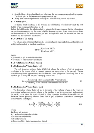
21. 12
Figure I- 7: Operating point
I.3.2.2. Artificial lift
I.3.2.2.1 Introduction
Over a period of time since the oil field begin producing the reservoir pressure decrease.
As a result the pressure becomes insufficient to bring up the fluid to the surface. In this case
artificial lift methods are employed allowing additional support.[3]
There are several common artificial lift techniques that have been developed and optimized
for different operating conditions such as rod pumps, electric submersible pumps and
hydraulic pumps) apart from gas lift.
I.3.2.2.2. Artificial lift forms
o Rod Pumps
Rod pumps (Figure I-8) are the most widely used in-land form of artificial lift. this unit is
made up of a surface unit connected to a down-hole with sucker rods. The main role of the
rod pump is creating a reciprocating motion in a sucker-rod string that connects to the down-
hole pump assembly. The conversion of this reciprocating motion to vertical fluid movement
is done by the intervention of a plunger and valve assembly. . This type of pump is used in
low flow rate wells (typically 5- 1500 of barrels of liquid per day).[3]

22. 13
Figure I- 8: Typical rod pump [3]
o Hydraulic Pumps
Hydraulic system transfer energy down-hole by pressurizing special power fluid, usually
water or light refined oil or pumped through well tubing or annulus to a subsurface pump,
which transmits the potential energy to produced fluids. So as shown in Figure I-9 the fluid is
injected into the pump and a small-diameter nozzle, where it becomes a low pressure, high
velocity jet. Produced fluid from the well-bore is mixed with the injected fluid and then goes
into an expanding-diameter diffuser. knowing that in the Bernoulli equation of state:
ℎ +
𝑉²
2𝑔
+
𝑃
𝜌𝑔
= 𝑐𝑜𝑛𝑠𝑡𝑎𝑛𝑡 II.6
when the pressure goes down the velocity goes up and vice versa. In the diffuser the fluid
underwent a velocity reduction and a pressure elevation. Common pumps consist of jets
(Venturi and orifice nozzles), reciprocating pistons, or less widely used rotating turbines.[6]
Figure I- 9: Hydraulic pump[4]
o Electric Submersible Pump
Electrical submersible pump is known as an economical and effective means of lifting
large volumes of fluid from deep wells under a variety of well conditions. Figure I-10
represents the ESP system .This system is characterized by it centrifugal pumps which contain
spinning impellers keyed on the shaft to put pressure on the surrounding fluid and leading it to
the surface. ESP is very versatile artificial lift method and can be found in operating

23. 14
environments all over the world. They can handle a very wide range of flow rates. The
remainder of this report details the components, sizing and operating principle.[3]
Figure I- 10: ESP system[4]
o Gas Lift
Gas Lift (Figure I-11) is a form of artificial lift where gas bubbles assist in lifting the oil
from the well. It's an additional high pressure gas injected either to the casing or tubing
annulus. The main purpose of gas lift technology is to reduce the well fluid density in order to
be capable to reach the surface. The process is as follows, the injected gas passes through a
valve where it mixes with the fluid and reduce its density. The reservoir pressure then lifts the
combined liquids to the surface where they are separated.[3][4]
Figure I- 11: Gas lift system[3]

24. 15
I.3.2.2.3. Advantages and disadvantages of different artificial lift technologies:
The advantages and disadvantages of the Major artificial lift methods are listed and compared
in Table I-1. Concerning electrical submersible pump advantages and limitations will be
treated in the next chapter.
Table I- 1: Advantages and Disadvantages of artificial lift technologies[4]
Artificial Lift Advantages Disadvantages
Rod Pumps
-Simple to operate
-Unit easy changed
-Can achieve -low BHFP
-Can lift high temperature
viscous oil
-Low intervention cost
-Can be installed in remote
locations without electricity
-Best understood by the field
personnel
-Pump wear with solids
(Sand, Wax...)
-Free gas reduce pump
efficiency
-heavy equipment for
offshore use
-Restricted flow and depth
-Potential wellhead leaks
Venturi Hydraulic Pump
-High volume
-Can use water as power
fluid
-Tolerate high well deviation
-Simplifies completions
significantly
-No moving parts, can
tolerate solids.
-High surface pressure
-Free gas reduce pump
efficiency
-Sensitive to change in
surface flow line-pressure
-Cavitations can occur with
high GOR
-High GOR impacts
performance
Gas Lift
-Solids tolerant
-large volume in high PI
wells
-Simple maintenance
-Unobtrusive
Surface location
-Tolerate high well deviation
-Tolerate high GOR reservoir
fluids
-Fairly low operation cost
-Flexibility: Can change
producing rate by adjusting
injection rates or/and
pressure.
-Lift gas may not be
available
-Not suitable for viscous
crude oil or emulsion
-Casing must withstand lift
gas pressure
I.4. Properties of reservoir fluids and phase behavior
I.4.1. Multiphase flow theory patterns and map
 Flow theory
The three components of the equation for predicting pressure losses are: elevation or static
components, friction component, acceleration component.
∆𝑃𝑡𝑜𝑡𝑎𝑙 = 𝐸𝑙𝑒𝑣𝑎𝑡𝑖𝑜𝑛 ℎ𝑦𝑑𝑟𝑜𝑠𝑡𝑎𝑡𝑖𝑐 + 𝐹𝑟𝑖𝑐𝑡𝑖𝑜𝑛 + 𝐴𝑐𝑐𝑒𝑟𝑎𝑡𝑖𝑜𝑛 I.7

25. 16
 Flow patterns
vertical flow
Figure I- 12: Vertical flow patterns
Figure I-12 represents the different vertical flow patterns:
 Bubble flow: Numerous yet discrete gas bubbles are dispersed in the continuous liquid
phase.
 slug flow: larger bubbles are formed with sizes similar to the tubing diameter. They are
separated from one another by slugs of liquids.
 churn flow: Higher velocities change the aspect of the flow; it becomes very unstable
which threatens to damage the pipe.
 wispy-annular flow: when the flow rates gets even higher the small droplets form clouds
of liquid in the center gaseous core.
 annular flow: Gas velocity exceeds the liquid's velocity. The liquid travels then in the
tube as thin film on the wall as the gas flows as a continuous phase.
horizontal flow
Figure I- 13: Horizontal flow patterns
Figure I-13 represents the different horizontal flow patterns:
 Bubble flow: Both gas and liquid move with the same velocity as the gas is dispersed as
bubbles that tend to accumulate at the top of the tubing.
 slug flow: At higher gas velocities in this regime occurs with its bigger elongated bubbles
and large vibrations caused by the liquid slugs between the bubbles.
 annular flow: At even greater gas velocities, the liquid forms a continuous annular film
that gets thicker at the bottom of the tube bubble point.

26. 17
 Stratified flow: At low liquid and gas velocities, the two phases are completely separated.
The liquid goes to the bottom as the gas goes to the top.
 Wavy flow: Increasing the fluids velocity in a stratified flow, waves are formed.
I.4.2. Bubble point.
The bubble point is defined as the pressure and temperature conditions at which the first
bubble of gas comes out of solution in oil.
Below the bubble point the solution of oil is saturated with gas, meaning that the oil contains
the maximum amount of gas that could it holds. So as the pressure drops along the way from
the bottom-hole to the well-head the gas will be separated from the solution as form of
bubbles and the oil will be unsaturated.
I.4.3. GOR (Gas Oil Ratio)
The oil gas ratio is the ratio between the volume of gas ( measured at standard conditions)
and the volume of oil at standard conditions.
𝐺𝑂𝑅 =
𝑉𝑔(𝑃𝑎𝑡𝑚, 60°𝐹)
𝑉𝑜(𝑃𝑎𝑡𝑚, 60°𝐹)
I.8
Where
Vg: volume of gas at standard conditions
Vo: volume of oil at standard conditions
I.4.4. FVF(Formation Volume Factor)
I.4.4.1. Formation Volume Factor (oil)
The oil formation volume factor (FVF/Bo) relates the volume of oil at stock-tank
conditions to the volume of oil at elevated pressure and temperature in the reservoir. Values
typically range from approximately 1.0 bbl/STB for crude oil systems containing little or no
solution gas to nearly 3.0 bbl/STB for highly volatile oils.
𝐵𝑜 =
𝑉𝑜𝑙𝑢𝑚𝑒 𝑜𝑓 𝑜𝑖𝑙 𝑖𝑛 𝑟𝑒𝑠𝑒𝑟𝑣𝑜𝑖𝑟, (Pr, 𝑇𝑟 𝑐𝑜𝑛𝑑𝑖𝑡𝑖𝑜𝑛)
𝑉𝑜𝑙𝑢𝑚𝑒 𝑜𝑓 𝑠𝑡𝑜𝑐𝑘 𝑡𝑎𝑛𝑘 𝑜𝑖𝑙 𝑖𝑛 𝑠𝑡𝑎𝑛𝑑𝑎𝑟𝑑 𝑐𝑜𝑛𝑑𝑖𝑡𝑖𝑜𝑛𝑠
I.9
I.4.4.2. Formation Volume Factor (gas)
The formation volume factor of gas is the ratio of the volume of gas at the reservoir
temperature and pressure to the volume at the standard or surface temperature and pressure
(ps and Ts). It is given the symbol Bg and is often expressed in either ((rcf) cubic feet of
reservoir volume per (scf) standard cubic foot of gas) or (barrels of reservoir volume per
standard cubic foot of gas).
𝐵𝑔 =
𝑉𝑅
𝑉𝑠𝑐
= (
𝑧𝑛𝑅𝑇
𝑝
) (
𝑃𝑠𝑐
𝑧𝑠𝑐 𝑛𝑅𝑇𝑠𝑐
) =
𝑃𝑠𝑐 𝑧𝑇
𝑇𝑠𝑐 𝑃
I.10
where
𝑉𝑅: Reservoir volume
𝑉𝑠 𝑐 : Volume in standard condition
𝑇: Reservoir Temperature
𝑛: Number of mole
𝑧: Compressibility factor (gas deviation factor)

27. 18
𝑧𝑠𝑐: Compressibility factor at standard condition
R: gas-law constant
𝑇𝑠𝑐: Temperature in standard condition
𝑃𝑠𝑐: Pressure in standard condition
𝑃𝑠𝑐
𝑇𝑠𝑐
=
14.696(𝑃𝑠𝑖)
519.67(°𝑅)
= 0.0282793
which implies
𝐵𝑔 = 0.0282793
𝑧𝑇
𝑃
(rcf/scf) I.11
The n divides out here because both volumes refer to the same quantity of mass.
Compressibility Factor
The compressibility factor is the same mass ratio of the real volume to the ideal volume,
which is a measure of the amount that the gas deviates from perfect behavior, is called the
super compressibility factor, sometimes shortened to the compressibility factor. It is also
called the gas deviation factor and given the symbol z. The gas deviation factor is by
definition the ratio of the volume actually occupied by a gas at a given pressure and
temperature to the volume it would occupy if it behaved ideally.
I.4.5. Water cut (WC)
Water cut is the ratio of water produced to the total volume of fluids produced: oil + water,
both volumes measured in standard conditions. It is expressed as a fraction in percent:
%𝑊𝑐 =
𝑉𝑤
𝑉𝑡
× 100 I.12
Where:
𝑉𝑤: the volume of produced water
𝑉𝑡: the total volume of produced fluid (oil + water)
% Wc: water cut percentage
I.4.6. Oil density
The density of a reservoir gas is defined as the mass of the gas divided by its reservoir
volume, so it can also be derived and calculated from the real gas law:
𝜌 𝑔 =
𝑚 𝑔
𝑉𝑅
=
𝑛𝑀𝑔
𝑧𝑛𝑅𝑇/𝑃
=
𝑛𝑀 𝑎𝑖𝑟 𝛾𝑔
𝑧𝑛𝑅𝑇/𝑃
=
28.967𝑃𝛾𝑔
𝑧𝑅𝑇
I.13
Where
𝑉𝑅: Reservoir volume
𝑇: Reservoir Temperature
𝑛: Number of mole
𝑧: Compressibility factor (gas deviation factor)
R: gas-law constant
𝑚 𝑔: Reservoir volume
𝑀𝑔: average molecular weight of gas mixture
𝑀 𝑎𝑖𝑟: molecular weight of air
𝜌 𝑔: density of gas

28. 19
𝛾𝑔: Specific gravity of gas
𝑚 𝑔: mass of gas
I.5. Conclusion
In this chapter Our interest was revolved around defining the petroleum production system
and explaining factors that involve in production optimization of the well, quoting the
example of inflow and outflow performance methods and artificial lift systems.

29. 20
Chapter II: Electrical Submersible Pump(ESP)
Objective
This chapter will detailed one of
production invention features to
transfer pressure to the fluid. So that
it will flow from the wellbore to the
surface at the desired rate.

30. 21
II.1. Introduction
II.1.1. General history of ESP
Unlike the other artificial lift methods electrical submersible pump was innovated and
improved by a Russian named Armais Arutunoff in the late 1910s.[5]
In 1911, Arutunoff started the company Russian Electrical Dynamo of Arutunoff (its acronym
REDA still being known all over the world) and developed the first electric motor that could
be operated submersed in an oil well.[5]
In 1926 the first installation of electrical submersible was operated in the El Dorado field in
Kansas.
II.1.2. General overview of ESP
The electrical submersible pump typically called ESP is a powerful and profitable means
of artificial lift representing technical characteristics in order to tolerate harsh environment
conditions and produces moderate to high amounts of well fluids in even extreme regions.
Electrical submersible pump deal with many problems which could be encountered when
producing such as high water cut, sand production, highly deviated wells, high bottom hole
temperature, abrasive and corrosive issues and high viscosity fluid.
ESP installation
ESP consists of an electrical alternative current motor, seal section, gas separator, multi-
stage centrifugal pump, power cable, surface control mechanism and transformers.
The classical or “conventional” installation is illustrated in Figure II-1 where the ESP unit is
run on the tubing string and is submerged in well fluids.[7]
The electric submersible motor is at the bottom of the unit just above the perforation zone.
It is connected to the protector (a.k.a. seal section) that ensures the unit safety through many
crucial functions. Overhead of the protector a pump intake or gas separator is settled which
allows well fluids to enter the centrifugal pump excluding from low quantities of free
gas(taken from the solution in the gas separator). Liquid is lifted up to the surface by the
multistage centrifugal pump, the heart of the ESP system. Surface equipments include a
junction box, surface electric cables and a control unit called switchboard that provides
measurement and control functions. The ESP unit receives AC electricity from a set of
transformers (not shown) which supply the required voltage by stepping up or down the
voltage available from the surface electric network.[7]

31. 22
Figure II- 1: Conventional ESP installation[7]
Theory of Operation
ESP constructional and operational features underwent a continuous evolution over the
years, their basic operational principle remained the same.[7]
The whole ESP systems function is to transform electrical power supplying from the
surface through copper resistant cables to head or potential energy in a form of pressure . ESP
units are typically installed over the perforation zone permitting fluid to flow from the
perforated area past the motor aiming to cool it. The motor generates the rotation of a shaft
which connects the seal protector and the pump by a mechanical coupling. So as the impellers
(the rotating part of the pump stage) are keyed to the shaft they will rotate in highly speed at
the same RPM (rotation per minute) of the motor shaft imparting Kinetic energy to the fluid
from a centrifugal force with the intervention of a stationary part of the pump called
diffuser.[3]
II.2. ESP components
ESP Systems include all the necessary components to transfer power from the surface,
convert the power into shaft rotation and impart energy to the produced fluids. A typically
ESP system includes:[3]
ESP down-hole components:
• Pump
• Gas Separator
• Seal
• Electric Motor
ESP Surface components:
• Junction box
• Power Cable
• Motor Controller
• Transformer

32. 23
II.2.1. ESP down-hole components
II.2.1.1 Pump
Introduction and purpose
Being the major part of the ESP system it's crucial to understand the operating principle of
the submersible pump. The main objective of a multistage centrifugal pump is to lift the fluid
from the bottom-hole up to the surface by converting the energy from rotational shaft into
centrifugal pump.
components
As shown in figure II.2 the submersible pump is made of the following basic components:
 Shaft, Impeller, Diffuser, Housing and Intake
Figure II- 2: ESP submersible pump cutaway[3]
Impeller
The impeller is locked to the shaft and rotates at the motor RPM. As the impeller rotates it
imparts centrifugal force on the production fluid. Figure II-3 is an illustration of an impeller
keyed to a shaft, and identifies key subcomponents of the impeller.[3]
Figure II- 3: Illustration of impeller and subcomponents[3]
Diffuser
The diffuser in the Figure II-4 turns the fluid into the next impeller and does not rotate.

33. 24
Figure II- 4: illustration cutaway of a diffuser[3]
pump stage
The pumps stage in Figure II-5 is a combination of an impeller and a diffuser.
Figure II- 5: Illustration of a pump stage[3]
pump Intake
The pump intake in Figure II-6 attaches to the lower end of the pump housing and provides
a passageway for fluids to enter and a flange to attach to the ESP seal.
Figure II- 6: Pump intake[3]
II.2.1.2 Gas separator
Introduction and purpose
Gas production has been a problem since the early days of oil production. It limited
production on many oil wells producing with pumps, It causes a gas locking and cavitations.
For this reason a gas separator should be designed to keep free gas for entering the pump.[3]
Components
The ESP Gas Separator in Figure II-7 is made up of the following major components:[3]

34. 25
- Gas Vent Port, Guide Vane, Inducer or High Angle Vane Auger (Patented), Separation
Chamber, Intake and a Shaft
Figure II- 7: Rotary gas separator[3]
II.2.1.3. Seal section
Introduction and purpose
The electric motor of the ESP system is completely sealed against the produced liquid in
order to prevent short-circuits and burning of the motor after it is contaminated with well
fluids.[7]
ESP motors must be kept open to their surroundings but at the same time must still be
protected from the harmful effects of well fluids. The main reason for this is that since the
motor must be filled up with a high dielectric strength oil, ESP motors operating at elevated
temperatures, if completely sealed, would burst their housing due to the great pressure
developed by the expansion of the oil.[7]
This is guaranteed by connecting a protector (a.k.a. seal) section between the motor and the
centrifugal pump.[7]
Seal sections perform the following vital functions:
• Isolates the clean motor oil from wellbore fluids to prevent contamination.[3]
• Couples the torque developed in the motor to the pump intake via the protector shaft.
• Provides a reservoir for the thermal expansion of the motor's oil.[4]
Seal section types
There are two main types of seal section:[4]
 Bag type protectors (positive seal): Designed to physically separate the well fluid and
motor oil.
 Labyrinth type protectors: Use the difference in specific gravity of the well fluid and the
motor oil to keep them apart even though they are in direct contact.
Components
Seal Sections are made up of the following major components:[3]
Mechanical Seals, Elastomer Bag(s), Labyrinth Chamber(s), Thrust Bearing, Heat Exchanger
Figure II-8 shows the construction of major components of a typical seal section.

35. 26
Figure II- 8: ESP combined seal section components[3]
II.2.1.4. Electrical motor
Introduction and purpose
The major and sole objective of a motor is the transformation of electrical energy into
motion that turns the shaft. This latter is connected through the seal and gas separator and
turns the pump impellers.[3]
components
Figure II-9 is an ESP Motor made up of the following major components:[3]
- Rotors, Stator, Shaft, Bearings, Insulated Magnet Wire, Winding Encapsulation, Rotor and
Stator Laminations, Housing, Thrust Bearing
Figure II- 9: ESP motor cutaway illustration[3]
II.2.2. ESP Surface components
II.2.2.1. Junction Box
A junction box (vent box) performs three functions. First, it provides a connection point for
the surface cable from the motor control panel to the power cable in the wellbore coming
from the wellhead . Second, it allows for any gas to vent that may have migrated through to
the power cable.
Finally, it provides accessible test point for electrically checking down-hole equipment.[4]

36. 27
During the installation of the junction box it's required to leave a minimum distance from
wellhead (35 ft) and from the switchboard (15ft).
II.2.2.2 Power cable
Banded to the tubing, the power cable is considered as an electrical power transfer means
from the surface to the down-hole motor. This cable must be of specific construction to
prevent mechanical damage, and able to retain its physical and electrical properties when
exposed to hot liquids and gasses in oil wells.[3][4]
The power cable is available on both flat or round construction. It consists of three copper
conductor wires extending from the top of the motor lead to the wellhead. The size of the
cable selected is based on amperage and voltage drop.[3][4]
II.2.2.3. Motor controller
The main function of the motor controller is primarily to protect the ESP motor by
measuring the surface current and voltage to avoid the underload and overload of the motor.
The controller also provides the capability to monitor performance of down-hole electrical
system(current, voltage, frequency, etc).
II.2.2.4. ESP variable speed drive
Variable speed drives (VSD) allows the variation of the ESP performance through the
motor speed control. As the shaft connects the motor to the protector and the pump VSD
modify also the pump impellers rotation speed. By allowing the pump speed to be varied, the
rate and/or head can be adjusted (depending on the application) with no modification of the
down-hole unit.[3]
Its numerous operational features make it one of the ESP assets such as:[3]
 Controlling motor speed can avoid heat failure (burning of the motor components)
 Control well drawdown
 Adjust ESPs with changing well conditions
 Decrease system stress at start up
II.2.2.5. Transformer
Since ESP equipments operation need a variable range of voltage from 250 volts up to
4000 volts depending on the power of the components. Voltage transformation is required
because electrical power is usually supplied to oilfield at a voltage of 6000 volts or higher.[3]
Transformers contain a substantial number of secondary voltage taps which allows a wide
range of output voltages. This is required in order to adjust the surface voltage to account for
cable voltage drop that occurs due to setting depths.[3]
II.2.3. ESP mainly support equipment
Most of well fields requires the involvement of some additional support equipment. For
example the most substantial ones are the wellhead, check valves, drain valve, backspin relay
and the centralizer. These equipments depends necessarily on the power available and the
conditions of the well.[3]
Wellhead
The main function of the wellhead is to support the weight of the subsurface equipment
and to maintain annular pressure of the well. It includes the pack-off generally known as the
tubing head bonnet. It's an additional element of sealing around the cable and the tubing. The
highest rated pack-off can resist pressure up to 5000 psi.[3]
Check Valve

37. 28
To avoid fluid falling down-hole during the shut off of the ESP system a check valve
should be installed. Without this equipment reverse rotation of the pump impellers and as a
result the reverse rotation of the pump and motor shaft may occur. In this case it cause a
electrical failure or mechanical damage to the equipment.[3]
Centralizer
Centralizers are used in ESP applications to set the equipment in the center of the wellbore.
This is chiefly practical in deviated wells to eliminate external damage and insure proper
cooling of the equipment..[3]
II.3. Performance of an ESP system
The Brake Horse Power is the power required to drive the pump which needs to cover the
sum of the energy that pump the well fluid and the energy losses arising in the pump and the
tubing due to friction. The mathematical relationship between head, capacity, efficiency and
brake horsepower is expressed as: [3]
𝐵𝐻𝑃 =
𝑄 × 𝐻 × 𝑆𝑝𝑒𝑐𝑖𝑓𝑖𝑐 𝐺𝑟𝑎𝑣𝑖𝑡𝑦
𝑃𝑢𝑚𝑝 𝐸𝑓𝑓𝑖𝑐𝑖𝑒𝑛𝑐𝑦
II.1
Where
Q: flow rate, bpd
H: head required, ft
The performance of ESP pumps is characterized by the pump performance curves which are
plotted in figure II-10 in the function of the pumping rate and represent:[7]
 the head developed by the pump
 the efficiency of the pump, and
 the mechanical power (brake horsepower) required to drive the pump when pumping
water.[7]
Figure II- 10: example performance curve of an ESP pump[7]
These curves are experimentally obtained with freshwater under controlled conditions at an
operating temperature of 60ºF. Tests on submersible pumps are made by driving the pump at
a constant rotational speed, usually 3,500 RPM for 60 Hz service. The actual performance
may be obtained by a simple correction using the Affinity Laws.[7]
Affinity Laws

38. 29
These are a couple of equations that link the actual speed of a centrifugal pump and its
performance parameters. There are in total three relationships:
 The flow rate is directly proportional to the pump's operating speed:
𝑄2 = 𝑄1
𝑁2
𝑁1
II.2
 The head is proportional to the square of the pump's operating speed:
𝐻2 = 𝐻1 (
𝑁2
𝑁1
)
2
II.3
 The brake horse power is proportional to the square of the pump's operating speed:
𝐵𝐻𝑃2 = 𝐵𝐻𝑃1 (
𝑁2
𝑁1
)
3
II.4
Where:
Q1: the first flow rate, bpd
Q2: the second flow rate, bpd
H1: the first head, ft
H2: the second head, ft
BHP1: the first brake horsepower, HP
BHP2: the second brake horsepower, HP
N1: first rotational speed, rpm
N2: second rotational speed, rpm
II.4. Evaluation of ESP components
II.4.1 ESP advantages
General advantages of using ESP units can be summed up as follows:
 Good efficiency over the widest range of production rate ( high to extremely high amount
of liquid)[5][4]
 Can achieve high production rates: the maximum is around 30,000 bpd from ft.[4][5]
 Suitable for both vertical and deviated well[5]
 Can operate reliably in onshore and offshore wells.[4]
 Can be flexible to accommodate changing conditions in time (PI, water cut Pwf, Pr, etc)
due to the Variable Speed Drive characteristic.[4]
 Can operate under tough conditions such as low bottom-hole pressure, high bottom-hole
temperature, high amount of corrosion and scale. [4][5]
 Surface equipment required a minimal space comparing with the other artificial lift
systems(sucker rod...) [5]
II.4.2. ESP disadvantages
The most known of ESP disadvantages are listed below:
 Expensive intervention cost: A pulling unit (heavy work-over rig) is required to retrieve
the failed ESP regardless of failed component. [4][5]
 Extremely high well temperature cable and motor insulation.[4]
 High solids and sand or abrasive materials may cause rapid equipment wear. For this
reason special abrasion-resistant materials are used and that increase the capital cost.[4]
[5]
 The presence of free gas at pump suction weakens the submersible pump's efficiency by
gas locking problems and can even totally prevent liquid production.[5]

39. 30
 ESP installation required a crucial availability of high voltage electrical power. [5]
 Production of high viscosity oils increases power requirements and reduces lift.[5]
II.5. Conclusion
In this chapter we intended to present the electrical submersible pump system. The main
objective was to thoroughly describe the ESP equipments with highlighting the particular
function of each one. We also mentioned the importance and the limitation of the ESP by
enumerating its advantages and disadvantages.

40. 31
Chapter III: Case study
Objective
This chapter includes a detailed
approach to follow in order to come
up with an electrical submersible
pump hand sizing and AutographPC
software.

41. 32
III.1. Hand sizing
III.1.1. The 9 steps procedure
The design of the Electric Submersible pump system follows these nine steps :
Step1: Basic Data
Collect and analyze all the well data that will be used for the design.[3][8]
Step2: Production Capacity
Determine the well productivity at the desired pump setting depth or determine the pump
setting depth at the desired production rate. [3][ 8]
Step3: Gas Calculation
Calculate the fluid volumes, including gas, at the pump intake conditions. [3][ 8]
Step4: Total Dynamic Head
Determine the required dynamic head and so the pump discharge requirement.[3][ 8]
Step5: Pump Type
For a given capacity and head select the pump type that will have the highest efficiency for
the desired flow rate. [3][ 8]
Step6: Optimum Size of Components
Select the optimum size of pump, motor and protector and check equipment limitations. [3][
8]
Step7: Electric Cable
Select the correct type and size of cable.[3][ 8]
Step8: Accessories and Optional Equipment
Select the motor controller, transformer, tubing head and optional equipment.[3][ 8]
Step9: The Variable Speed Pumping System
For additional operational flexibility, select the variable speed submersible pumping system.
Reliable information or data must be available to design a submersible pumping unit.
Although if the information, especially that pertaining to the well’s capacity, is poor, the
design will not be accurate and will be almost marginal. Bad data often results in a misapplied
pump and costly operation.[3][ 8]
A misapplied pump may operate outside the recommended range, overload or under-load the
motor or drawdown the well at a rapid rate which may result in formation damage. On the
other side, the pump may not be large enough to provide the desired production rate.[3][ 8]
The selection and design procedure may vary significantly depending on the well fluid
properties. The three major types of ESP applications are:[3][ 8]
 High water-cut wells producing fresh water or brine.
 Wells with multi-phase flow (high GOR).
 Wells producing highly viscous fluids.
Following is list of the data required:
A) Wells Data
 Casing or liner size and weight.
 Tubing size, type and thread (condition).
 Perforated or open hole interval.
 Pump setting depth (measured and vertical).[3][ 8]
B) Production Data
 Wellhead tubing pressure.
 Wellhead casing pressure.
 Present production rate.
 Producing fluid level.

42. 33
 Static fluid level and/or static bottom-hole pressure.
 Datum point.
 Bottom-hole temperature.
 Desired production rate.
 Gas-oil ratio.
 Water cut.[3][ 8]
C) Well Fluid Conditions
 Specific gravity of water.
 Oil API or specific gravity.
 Specific gravity of gas.
 Bubble-point pressure and temperature.
 PVT data.[3][ 8]
D) Power Sources
 Available primary voltage.
 Frequency.
 Power source capabilities.[3][ 8]
E) Possible Problems
 Sand Production.
 Corrosion.
 Paraffin.
 Emulsion.
 Gas.etc…[3][ 8]

43. 34
III.1.1.1 Basic data
Table III- 1: Pump Design data for 3 wells
Well name Cherouk 1
Shaheen 1 Badr 6
Well data
API casing
9 5/8"OD(8.681"
ID) 47#/ft
9 5/8"OD(8.681"
ID) 47#/ft
9 5/8"OD(8.681"
ID) 47#/ft
API Tubing
3 1/2"OD(2.991"
ID) 9.3#/ft
3 1/2"OD(2.991"
ID) 9.3#/ft
3 1/2"OD(2.991"
ID) 9.2#/ft
Well Type
Cased and
perforated hole
Cased and
perforated hole
Cased and
perforated hole
Perforation intervals
From 11023.488 ft
to 11305.63 ft
4 zones of perfo:
From 10331 ft to
10492 ft
From 11040 ft to
11335 ft
From 11381 ft to
11492 ft
From 11584 ft to
11686 ft
From 10724,6 ft
to 11568,1 ft
Reservoir data(from test and production data)
Present Production rate 1965 BFPD 1113 BFPD 1432 BFPD
Reservoir pressure 4200 psi 2285 psi 3070 psi
Current Bottom-hole
flowing pressure
3091 psi for 1965
BPD
1193.82 psi for
1065 BPD
1608.78 psi for
1376 BFPD
Producing GOR 1577 scf/stb 800 scf/stb 647 scf/stb
Water cut 89.5% 70% 24%
Oil API Gravity 42.3° 40° 41°

44. 35
Bottom Hole temperature 197°F 198°F 195.8°F
Water specific gravity 1.2 1.2 1.2
Gas specific gravity 0.84 0.825 0.82
PVTdata
Solution gas oil
ratio (Rs)
To be determined from design
Oil FVF (Bo) 1.87 rb/stb 1.43 rb/stb 1.43 rb/stb
Bubble
point
Pressure
4080 psi 1985 psi 1969 psi
Temperature
197 °F 199.4 °F 211 °F
Production
Index(PI)
1.8 bbl/day/psi 1.02 bbl/day/psi 0.98bbl/day/psi
Specifications
Desired Production rate 3000 bpd 1623 bpd 1660 bpd
Desired pump setting
depth
10170.48 ft 10170.48 ft 10170.48 ft
Desired PIP: Pump Intake
Pressure
To be determined within design
Required wellhead
pressure
220 psi 162 psi 184 psi
GOR through pump To be determined within design
Required electric power To be determined within design

45. 36
Desired pump series To be determined within design
Desired pump type To be determined within design
Motor type To be determined within design
Special
problems
Sand No No No
Scale
Deposit
No No No
Corrosion No No No
Paraffin No No No
H2S No No No
III.1.1.2. Production capacity
In this step, we will determine the well productivity at the test pressure and production. In
this case of study the pump setting depth PSD and the desired production rate Qd are given as
well as the production index PI.
The pump intake pressure can for instance be calculated. The pump intake pressure is
necessary to properly feed the pump and prevent cavitation or gas locking.
We will determine firstly the Pressure at well face Pwf at the desired production rate:
𝑃𝐼 =
𝑄𝑑
𝑃𝑟 − 𝑃𝑤𝑓
III.1
So:
𝑃𝑤𝑓 = 𝑃𝑟 − (
𝑄𝑑
𝑃𝐼
) III.2
Where
𝑃𝑤𝑓: Pressure at well face (bottom hole flowing pressure)
𝑃𝑟: reservoir pressure
𝑄𝑑: Desired flow-rate
𝑃𝐼: Productivity index
The pump intake pressure can be determined by correcting the flowing bottom-hole
pressure for the difference in pump setting depth and the datum point and by considering the
friction losses in the annulus.
As there is a mixed solution of water and oil in the produced fluids, it’s required to calculate
a composite specific gravity of the produced fluids. To find the composite specific gravity:
𝐴𝑑𝑗𝑢𝑠𝑡𝑒𝑑 𝑊𝑎𝑡𝑒𝑟 𝑠𝑝𝑒𝑐𝑖𝑓𝑖𝑐 𝐺𝑟𝑎𝑣𝑖𝑡𝑦 = 𝑊𝑐 × 𝑆𝐺𝑤 III.3
Where
WC: water cut
SGw: Specific gravity of water
III.4

46. 37
𝑂𝑖𝑙 𝑆𝑝𝑒𝑐𝑖𝑓𝑖𝑐 𝐺𝑟𝑎𝑣𝑖𝑡𝑦 =
141.5
°𝐴𝑝𝑖 + 131.5
𝐴𝑑𝑗𝑢𝑠𝑡𝑒𝑑 𝑂𝑖𝑙 𝑆𝑝𝑒𝑐𝑖𝑓𝑖𝑐 𝐺𝑟𝑎𝑣𝑖𝑡𝑦 = (1 − 𝑊𝑐) × 𝑆𝐺𝑜𝑖𝑙 III.5
Where
SGoil: specific gravity of oil
so:
𝑆𝐺𝑙𝑖𝑞𝑢𝑖𝑑 = 𝐴𝑊𝑆𝐺 + 𝐴𝑂𝑆𝐺 III.6
Where
SGliquid: Composite specific gravity of liquid
AWSG: Adjusted Water Specific Gravity
AOSG: Adjusted Oil Specific Gravity
The pressure due to the difference of perforation depth and pump setting depth can be
determined as follows:
𝑃𝑆𝐼 =
ℎ𝑒𝑎𝑑(𝑓𝑡) × 𝑆𝐺𝑙𝑖𝑞𝑢𝑖𝑑
2.31 (
𝑓𝑡
𝑝𝑠𝑖
)
III.7
where
ℎ𝑒𝑎𝑑(𝑓𝑡)=𝑑𝑎𝑡𝑢𝑚 𝑑𝑒𝑝𝑡ℎ(𝑓𝑡)−𝑝𝑢𝑚𝑝 𝑑𝑒𝑝𝑡ℎ(𝑓𝑡) III.8
Therefore the pump intake pressure without friction PIP will be:
𝑃𝐼𝑃 = 𝑃𝑤𝑓 − 𝑃𝑆𝐼 III.9
The friction to the intake is calculated as follows:
𝐹𝑟𝑖𝑐𝑡𝑖𝑜𝑛 𝑡𝑜 𝑡ℎ𝑒 𝑖𝑛𝑡𝑎𝑘𝑒(𝑓𝑡) = 𝐹𝐿 × (𝑑𝑎𝑡𝑢𝑚 𝑑𝑒𝑝𝑡ℎ − 𝑝𝑢𝑚𝑝 𝑠𝑒𝑡𝑡𝑖𝑛𝑔 𝑑𝑒𝑝𝑡ℎ) III.10
Where
FL: Friction Loss
This value of friction loss is determined by use of the chart of friction losses in API tubular
(Appendix A.1.a).
As the pump is setting at liner level (7"OD) and the desired flow rate of the three wells
(Cherouk1, Shaheen1 and Badr 6) are as follows 3000 bbl/day, 1623 bbl/day,1660 bbl/day,
we noticed that the vertical lines don't across the oblique one (Appendix A.1.a). In view of
that fact we assumed that the friction losses in the three cases is the minimum value of the
chart.
So the pump intake pressure PIP w/f considering the pressure losses is
𝑃𝐼𝑃 𝑤𝑓 = 𝑃𝐼𝑃 − 𝑓𝑟𝑖𝑐𝑡𝑖𝑜𝑛 𝑡𝑜 𝑡ℎ𝑒 𝑖𝑛𝑡𝑎𝑘𝑒 III.11

47. 38
Table III- 2: Pump intake pressure calculation steps
Well name Cherouq1 Shaheen1 Badr6
Bottom-hole flowing
pressure at the
desired rate
Pwf(psi)
2533.33 693.713 1376.391
Adjusted Water
specific gravity
1.074 0.84 0.288
°API 42.3 40 41
Water Cut WC(%) 89.5 70 24
Specific Gravity of
oil SGoil
0.814 0.825 0.82
Specific Gravity of
Water SGw
1.2 1.2 1.2
Adjusted oil specific
gravity
0.085 0.247 0.623
Specific Gravity of
Liquid SGliquid
1.159 1.087 0.911
Datum depth(ft) 11164.56 11146.35 11146.35
Pump depth(ft) 10170.48 10170.48 10170.48
Head(ft) 994.08 975.87 975.87
PSI 498.97 459.43 385.034
Pump Intake
Pressure without
Friction PIPw/o
Friction
2034.362 psi 234.285 psi 991.358 psi
Friction factor(ft) 0.01 0.01 0.01
Pressure due to
friction (ft)
9.94 9.7587 9.7587
Pressure due to
friction (psi)
4.99 4.594 3.85
Pump Intake
Pressure with
Friction PIPw/f(psi)
2029.371 229.69 987.508

48. 39
III.1.1.3. Gas calculation
In this third step, we need to determine the total fluid mixture inclusive of water, oil and
free gas that will enter the pump.[3][8]
1) We will determine first of all the solution Gas Oil Ratio (Rs) at the pump intake, for this
purpose we will use the Standing’s approach or correlation and substitute the pump intake
pressure for the bubble pressure in the following formula:
𝑅𝑠 = 𝑆𝐺𝑔 × (
𝑃𝑏
18
×
100.0125×°𝐴𝑃𝐼
100.00091×𝑇(°𝐹)
)
1.2048
III.12
where:
T: reservoir temperature.
SGgas: specifig gravity of gas.
Pb: bubble point pressure
2) Since the oil formation volume factor is given no need to determine it using the Standing’s
approach. We will assume that it will not change remarkably otherwise we could use the
following formula to check the exactitude of our data:
𝐵𝑜 = 0.972 + 0.000147 × {5.61 × 𝑅𝑠 × ((
𝑆𝐺𝑔𝑎𝑠
𝑆𝐺𝑜𝑖𝑙
)
0.5
) + 1.25 × (1.8𝑡 + 32)}
1.175
III.13
Where:
t: Bottom-hole Temperature, °C
Rs: solution gas oil ratio at pump intake
SGoil: specific gravity of oil
SGgas: specific gravity of gas
Bo is measured in (rb/stb) where rb is barrel at reservoir conditions
3) Determine the gas volume factor Bg as follows:
𝐵𝑔 = 5.04 ×
𝑍 × 𝑇
𝑃
III.14
Where:
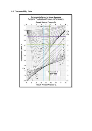
Z: Gas compressibility factor
T: Bottom-hole temperature degrees Rankin (460+°F)
P: Submergence pressure, psi (reservoir pressure)
The compressibility factor or the deviation factor Z is not given in the well data table so we
should calculate it.
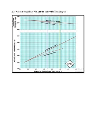
Based on the gas specific gravity we determine as a first step the pseudo-critical pressure and
temperature referring to the (Appendix A.2)
After determining the Pseudo-critical Temperature Tpc(°R) and the Pseudo-critical Pressure
Ppc (psi) we calculate the Pseudo-reduced Temperature Tpr(°R) and the Pseudo-reduced
Pressure Ppr(psi).
𝑃𝑝𝑟 =
𝑃𝑟
𝑃𝑝𝑐
III.15

49. 40
𝑇𝑝𝑟 =
𝑇
𝑇𝑝𝑐
III.16
where:
T: bottom-hole temperature, °R
Pr: reservoir pressure
With these two parameters the deviation factor can be graphically determined from (Appendix
A.3)
4) Next, we will determine the total volume of fluids and the percentage of free gas released
at the pump intake:
a) Using the producing GOR and the oil volume at the surface, we determine the total volume
of gas Tg(mcf):
𝑇𝑔 =
𝐵𝑂𝑃𝐷 × 𝐺𝑂𝑅
1000
III.17
where:
Tg: total volume of gas at the surface
BOPD: barrel of oil per day
GOR: producing gas oil ratio (at the surface)
mcf is a traditional unit of volume equal to 1000 cubic foot
b) Using the solution GOR (Rs) at the pump intake, we determine the volume of solution
gas SOLg(mcf):
𝑆𝑂𝐿𝑔 =
𝐵𝑂𝑃𝐷 × 𝑅𝑠
1000
III.18
where:
SOLg: the volume of solution gas (gas dissolved in the gas and oil solution)
BOPD: barrel of oil per day
Rs: solution gas oil ratio (at pump intake)
c) The difference represents the volume of free gas (Fg) released from solution by the
decrease in pressure from bubble point pressure Pb to pump intake pressure PIP
𝐹𝑔 = 𝑇𝑔 − 𝑆𝑂𝐿𝑔 III.19
d) The volume of oil (Vo) at the pump intake:
𝑉𝑜 = 𝐵𝑂𝑃𝐷 × 𝐵𝑜 III.20
e) The volume of free gas (Vg) at the pump intake:
𝑉𝑔 = 𝐹𝑔 × 𝐵𝑔 III.21
f) The volume of water (Vw) at the pump intake:

50. 41
𝑉𝑤 = 𝐵𝑊𝑃𝐷 × 𝐵𝑤 III.22
Where:
BWPD: barrel of water per day
Bw: water formation volume factor
we suppose that Bw =1
g) The total volume (Vt) of oil, water and gas at the pump intake can be now determined:
𝑉𝑡 = 𝑉𝑤 + 𝑉𝑔 + 𝑉𝑜 III.23
h) The ratio or the percentage of free gas %Fg present at the pump intake to the total of fluid
is:
%𝐹𝑔 =
𝑉𝑔
𝑉𝑡
III.24
Actually, as long as the gas remains in solution, the pump behaves normally and at high
performance as if it’s pumping a liquid of low density. However, the pump begins producing
lower head than required as the gas/oil ratio (at pumping conditions) increases beyond a
“critical” value (usually about 10 % to 15 % of total fluid volume). If the percentage of free
gas to the total of fluid volume is less than 10 %, the pump can withstand this and the
performance decreases slightly but over 10 %, the performance of the pump decreases
significantly. The main reason for this is that it will occur great slippage between the two
phases present liquid and gas leading to decrease of the pump intake pressure an. Accordingly
the phenomenon of cavitation appears and unfortunately the head required couldn't be
achieved, a separator must be installed to deal with this problem.[3][8]
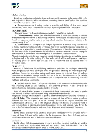
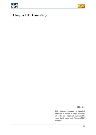
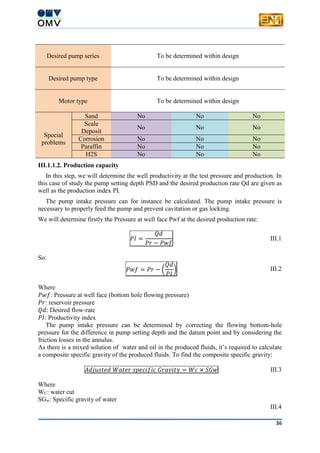
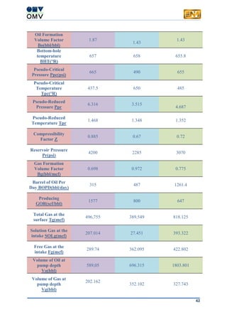
Table III- 3: Free gas calculation steps
Well name Cherouq1 Shaheen1 Badr6
Specific Gravity of
Gas SGgas
0.84 1.08 0.99
Pump Intake
Pressure PIP(psi)
2029.371 229.69 987.508
°API 42.3 41 40
Bottom-hole
Temperature
BHT(°F)
197 198 195.8
Solution GOR
Rs(scf/stb)
657.188 56.376 311.814
Specific Gravity of
Oil SGoil
0.814 0.825 0.82
Bottom-hole
temperature(°C)
91.66 92.22 91

51. 42
Oil Formation
Volume Factor
Bo(bbl/bbl)
1.87
1.43
1.43
Bottom-hole
temperature
BHT(°R)
657 658 655.8
Pseudo-Critical
Pressure Ppc(psi)
665 490 655
Pseudo-Critical
Temperature
Tpc(°R)
437.5 650 485
Pseudo-Reduced
Pressure Ppr
6.316 3.515
4.687
Pseudo-Reduced
Temperature Tpr
1.468 1.348 1.352
Compressibility
Factor Z
0.885 0.67 0.72
Reservoir Pressure
Pr(psi)
4200 2285 3070
Gas Formation
Volume Factor
Bg(bbl/mcf)
0.698 0.972 0.775
Barrel of Oil Per
Day BOPD(bbl/day)
315 487 1261.4
Producing
GOR(scf/bbl)
1577 800 647
Total Gas at the
surface Tg(mcf)
496,755 389.549 818.125
Solution Gas at the
intake SOLg(mcf)
207.014 27.451 393.322
Free Gas at the
intake Fg(mcf)
289.74 362.095 422.802
Volume of Oil at
pump depth
Vo(bbl)
589,05 696.315 1803.801
Volume of Gas at
pump depth
Vg(bbl)
202.162
352.102 327.743

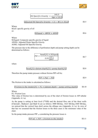
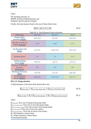
52. 43
Volume of Water at
pump depth
Vw(bbl)
2685
1136.178 398.337
Total Volume at
pump depth Vt(bbl)
3476.212 2184.595 2529.881
Percentage of Free
Gas at pump depth
Fg(%)
5,81% 16.11% 12.94%
In our case of study the percentage of free gas is less than 10% by volume just for
Cherouq1, it would have little effect on the pump performance therefore, a gas separator is not
required. But for Shaheen 1 and Badr 6 we should install a gas separator because the
percentage of free gas is higher than 10%. The gas separator should have the same diameter as
the pump, that's means the same series. Our choice is based on the series of the pump.(See
ESP Design summary table.
III.1.1.4. Total dynamic head
This step consists on the calculation of the total dynamic head required to pump the desired
capacity. The total pump head refers to feet of liquid being pumped and is calculated to be the
sum of:
 Net well lift (dynamic lift).
 Well tubing friction losses.
 Wellhead discharge pressure converted to footage.[3][10]
The simplified equation is as follows:
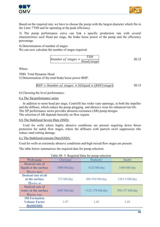
𝑇𝐷𝐻 = 𝐻𝑑 + 𝐹𝑡 + 𝑃𝑑 III.25
Where:
TDH: Total dynamic head in feet delivered by the pump when pumping the desired volume.
Hd: Vertical distance in feet between the wellhead and the estimated producing fluid level at
the expected capacity (Figure III-1).
Ft: The head required to overcome the friction losses in tubing.
Pd: The head required to overcome friction in the surface pipe, valves etc… and to overcome
also elevation changes between wellhead and the tank.

53. 44
Figure III- 1: Total dynamic head[10]
1) Determination of Hd:
The vertical distance between the estimated producing fluid level and the surface (Hd) is
determined as follows:[3][8]
𝐻 𝑑 = 𝑃𝑆𝐷 − (
𝑃𝐼𝑃 × 2.31
𝑆𝐺𝑙𝑖𝑞𝑢𝑖𝑑
) III.26
Where:
PSD: pump setting depth, ft
PIP: pump intake pressure, psi
SGliquid: specific gravity of the liquid
2) Determination of the tubing friction losses:
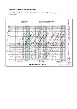
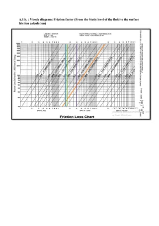
This value is determined by using the chart of friction losses in API tubular (Appendix A.1.b)
𝐹𝑡 =
𝑃𝑢𝑚𝑝 𝑠𝑒𝑡𝑡𝑖𝑛𝑔 𝑑𝑒𝑝𝑡ℎ × 𝑓𝑟𝑖𝑐𝑡𝑖𝑜𝑛 𝑓𝑎𝑐𝑡𝑜𝑟
1000
III.27
The discharge pressure head (desired wellhead pressure ) is determined as follows:
𝑃𝑑(𝑓𝑡) =
𝐷𝑊𝐻𝑃(𝑝𝑠𝑖) × 2.31(
𝑓𝑡
𝑝𝑠𝑖)
𝑆𝐺𝑙𝑖𝑞𝑢𝑖𝑑
III.28

54. 45
where
Pd: discharge pressure, ft
DWHP: desired wellhead pressure, psi
SGliquid: specific gravity of liquid
Finally, the total dynamic head is the sum of these three terms:
𝑇𝐷𝐻 = 𝐻𝑑 + 𝐹𝑡 + 𝑃𝑑 III.29
Table III- 4: Total Dynamic head calculation
Well name Cherouq1 Shaheen1 Badr6
Pump intake
pressure PIP(ft)
4043.039 487.885 2502.844
Specific Gravity of
liquid SGliquid
1,159 1.087 0.911
Net Dynamic Lift
Hd(ft)
6127.44 9682.594 7667.635
Friction factor 49 16 16.5
Tubing friction
losses Ft(ft)
498.353 162.72 167.813
Desired Well-Head
Pressure
DWHP(psi)
220 162 184
Discharge Pressure
Pd(ft)
438.298 314.103 466.349
Total Dynamic
Head TDH(ft)
7064.091 10189.426 8301.79
III.1.1.5. Pump selection
1) Determination of the down-hole desired flow rate:
𝑄 𝑑𝑜𝑤𝑛−ℎ𝑜𝑙𝑒 = 𝑄 𝑜𝑖𝑙 𝑎𝑡 𝑡ℎ𝑒 𝑑𝑜𝑤𝑛−ℎ𝑜𝑙𝑒 + 𝑄 𝑤𝑎𝑡𝑒𝑟 𝑎𝑡 𝑡ℎ𝑒 𝑑𝑜𝑤𝑛−ℎ𝑜𝑙𝑒. III.30
𝑄 𝑑𝑜𝑤𝑛−ℎ𝑜𝑙𝑒 = 𝐵𝑜 × 𝑄 𝑜𝑖𝑙 𝑎𝑡 𝑡ℎ𝑒 𝑠𝑢𝑟𝑓𝑎𝑐𝑒 + 𝐵 𝑤 × 𝑄 𝑤𝑎𝑡𝑒𝑟 𝑎𝑡 𝑡ℎ𝑒 𝑠𝑢𝑟𝑓𝑎𝑐𝑒 III.31
where
Q down-hole: flow rate of liquid at the pump intake
Q oil at the down-hole: Flow rate of oil at the pump intake
Q water at the down-hole: Flow rate of water at the pump intake
Q oil at the surface: Flow rate of oil at the surface
Q water at the surface : Flow rate of water at the surface
Bo: Oil formation volume factor
Bw: Water formation volume factor
2) choosing the pump:

55. 46
Based on the required rate, we have to choose the pump with the largest diameter which fits in
the Liner 7"OD and be operating at the peak efficiency.
3) The pump performance curve can link a specific production rate with several
characteristics such Head per stage, the brake horse power of the pump and the efficiency
percentage.
4) Determination of number of stages:
We can now calculate the number of stages required:
𝑁𝑢𝑚𝑏𝑒𝑟 𝑜𝑓 𝑠𝑡𝑎𝑔𝑒𝑠 =
𝑇𝐷𝐻
𝐻𝑒𝑎𝑑/𝑠𝑡𝑎𝑔𝑒
III.32
Where
TDH: Total Dynamic Head
5) Determination of the total brake horse power BHP:
𝐵𝐻𝑃 = 𝑁𝑢𝑚𝑏𝑒𝑟 𝑜𝑓 𝑠𝑡𝑎𝑔𝑒𝑠 × 𝑆𝐺𝑙𝑖𝑞𝑢𝑖𝑑 × (𝐵𝐻𝑃/𝑠𝑡𝑎𝑔𝑒) III.33
6) Choosing the level performance:
6.a The Xp performance series
In addition to more head per stage, Centrilift has wider vane openings, in both the impeller
and the diffuser, which reduce the pump plugging and abrasive wear for enhanced run life.
The XP performance series provides abrasion resistance (AR) pump designs
The selection of AR depends basically on flow regime
6.b The Stabilized Severe Duty (SSD):
Used for wells where highly abrasive conditions are present requiring down thrust
protection for radial flow stages, where the diffusers with particle swirl suppression ribs
reduce sand cutting damage.
6.c The Stabilized extreme Duty(SXD):
Used for wells at extremely abrasive conditions and high mixed flow stages are present.
The table below summarizes the required data for pump selection.
Table III- 5: Required Data for pump selection
Well name Cherouq1 Shaheen1 Badr6
Desired rate of
liquid at the surface
Qsurface liquid
3000 bbl/day 1623 bbl/day 1660 bbl/day
Desired rate of oil
at the surface
Qsurface oil
315 bbl/day 486.934 bbl/day 1261.4 bbl/day
Desired rate of
water at the surface
Qsurface water
2685 bbl/day 1123.178 bbl/day 398.337 bbl/day
Oil Formation
Volume Factor
Bo(bbl/bbl)
1.87 1.43 1.43

56. 47
Water Formation
Volume Factor
Bw(bbl/bbl)
1 1 1
Desired rate of oil
at the pump intake
Qoil down-hole
589.05 bbl/day 696.315 bbl/day 1803.801 bbl/day
Desired rate of
water at the pump
intake Qwater down-hole
2685 bbl/day 1123.178 bbl/day 398.337 bbl/day
Desired rate of
liquid at the pump
intake Qliquid down-hole
3274.05 bbl/day 1832.494 bbl/day 2202.138 bbl/day
Desired rate of
liquid at the pump
intake Q liquid down-
hole
520 M3
/day 291 M3
/day 350 M3
/day
Casing OD 9 5/8" 9 5/8" 9 5/8"
Tubing OD 3.1/2" 3.1/2" 3.1/2"
Liner OD 7" 7" 7"
After a thorough checking we choose from the Centrilift pump catalog[6]:
 Centurion pump 538 series: P37 (Figure III-2) For Cherouq 1
 Centurion pump 538 series: P23 (Figure III-3) For Shaheen 1
 Centurion pump 538 series: G31 (Figure III-4) For Badr 6
8) Pump performance curves

57. 48
Figure III- 2: Pump performance curve 538 series P37 Centurion pump[6]
Figure III- 3: Pump performance curve 538 series P23 Centurion pump[6]

58. 49
Figure III- 4: Pump performance curve 538 series G31 Centurion pump[6]
a) Pump's stage and housing number
Referring to (Appendix B.1) we choose the number of stages and housing defining each pump
based on number of stage calculated theoretically.
Table III- 6: Pump specifications
Well name Cherouq1 Shaheen 1 Badr6
Desired rate of
liquid at the pump
intake Q liquid down-
hole
520 M3
/day 291 M3
/day 350 M3
/day
Pump series P37 538-SSD series P23 538- SSD series G31 538-SXD series
Pump OD 5.38" 5.38" 5.38"
Operation range
From 330 to 635
M3
/day at 50.0 Hz
From 160 to 370
M3
/day at 50.0 Hz
From 240 to 580
M3
/day at 50.0 Hz
Efficiency(%) 68 % 64 % 46.66 %

59. 50
Ft/stage 11.5 m 12.25 m 13.1 m
Ft/stage 37.73 ft 40.19 ft 42.978 ft
TDH 7064.091 10189.426 8301.797
Number of stages
calculated
188 254 193
Number of stages
required
the values above go well beyond the technical data sheet reference
values.(Appendices: B.1.a, B.1.b and B.1.c)
For this reason we have to choose two or three housing and summing
its corresponding number of stages to ensure reaching the number
required.
189 254 192
Housing required
2 (N°16 and N°6)
Appendix B.1.a
2 (N°17 and N°5)
Appendix B.1.b
2 (N°18 and N°10)
Appendix B.1.c
Brake Horse Power
per stage
1 KW 0.65 KW 1.15 KW
Brake Horse Power
per stage
1.34 HP 0.872 HP 1.542 HP
Total Brake Horse
Power
293.651 HP 221.448 HP 269.839 HP
Shaft Diameter 0.875" 0.875" 0.875"
Level performance XP performance XP performance XP performance
III.1.1.6. Seal section selection
Normally the seal section series should be the same as that of the pump, although, there are
exceptions and special adapters are available to connect the units together. In our case study,
we will assume that the seal section and the pump are of the same series.[3]
The horsepower requirement for the seal section is based upon the total dynamic head
produced by the pump.[3]
We considered that the seal section and pump are of the same series which is 538[9].

60. 51
The GSB3 model is chosen for Cherouq 1 and Shaheen 1 wells (Appendix B.2.a) and
FSFB3 model is picked for Badr 6 well (Appendix B.2.b). The horsepower required for the
seal section is based upon the total dynamic head produced by the pump such indicated from
the chart below: Figure III-5.[3]
Figure III- 5: Horsepower VS Total dynamic head in feet[3]
The table below shows the Seal horsepower estimation
Table III- 7: Seal horsepower estimation
Well name Cherouq1 Shaheen1 Badr6
Total Dynamic
Head (ft)
7064.091 10189.426 8301.797
Seal horsepower
(HP)
3.4 3.45 3.6
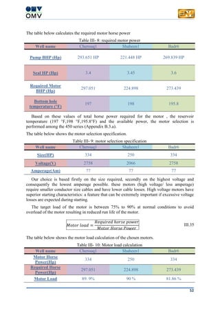
III.1.1.7 Motor selection
The most important criteria for motor selection are :
 Horsepower
 Voltage
 Amperage
 Load
 BHT
The brake horse power required for the motor is calculated before, we have to take into
account the horse power needed for the seal section to calculate the total horse power needed
for the motor.
𝑚𝑜𝑡𝑜𝑟 𝐵𝐻𝑃 = 𝑝𝑢𝑚𝑝 𝐵𝐻𝑃 + 𝑠𝑒𝑎𝑙 𝐻𝑃 III.34

61. 52
The table below calculates the required motor horse power
Table III- 8: required motor power
Well name Cherouq1 Shaheen1 Badr6
Pump BHP (Hp) 293.651 HP 221.448 HP 269.839 HP
Seal HP (Hp) 3.4 3.45 3.6
Required Motor
BHP (Hp)
297.051 224.898 273.439
Bottom hole
temperature (°F)
197 198 195.8
Based on these values of total horse power required for the motor , the reservoir
temperature (197 °F,198 °F,195.8°F) and the available power, the motor selection is
performed among the 450 series (Appendix B.3.a).
The table below shows the motor selection specification.
Table III- 9: motor selection specification
Well name Cherouq1 Shaheen1 Badr6
Size(HP) 334 250 334
Voltage(V) 2758 2066 2758
Amperage(Am) 77 77 77
Our choice is based firstly on the size required, secondly on the highest voltage and
consequently the lowest amperage possible. these motors (high voltage/ less amperage)
require smaller conductor size cables and have lower cable losses. High voltage motors have
superior starting characteristics: a feature that can be extremely important if excessive voltage
losses are expected during starting.
The target load of the motor is between 75% to 90% at normal conditions to avoid
overload of the motor resulting in reduced run life of the motor.
𝑀𝑜𝑡𝑜𝑟 𝑙𝑜𝑎𝑑 =
𝑅𝑒𝑞𝑢𝑖𝑟𝑒𝑑 ℎ𝑜𝑟𝑠𝑒 𝑝𝑜𝑤𝑒𝑟
𝑀𝑜𝑡𝑜𝑟 𝐻𝑜𝑟𝑠𝑒 𝑃𝑜𝑤𝑒𝑟
III.35
The table below shows the motor load calculation of the chosen motors.
Table III- 10: Motor load calculation
Well name Cherouq1 Shaheen1 Badr6
Motor Horse
Power(Hp)
334 250 334
Required Horse
Power(Hp)
297.051 224.898 273.439
Motor Load 89. 9% 90 % 81.86 %

62. 53
We can conclude that all motor load values are between 75% and 90% that confirms our
choice.
III.1.1.8. Power cable selection
Many parameters are involved in the choice of the power cable namely, amperage (voltage
drop), conductor temperature (insulation material), insulation voltage rating, gas handling
(decompression protection), corrosive properties of well fluid, available space (casing
clearance).
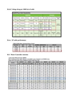
A) Amperage (Voltage Drop)
Line loss is the normal reduction in available voltage after long distance transmission.
High temperatures impede the ability of the conductor to transmit voltage (resistance).
Voltage drop refers to voltage losses due to distance and temperatures.[3][8]
The conductor size is measured by American Wire Gauge(#AWG). The size goes from 1
to 6 with 1 for the largest size, however the voltage drop increases with the largest diameter.
For this reason it is recommended to select the tightest allowed cable size.
The Voltage Drop per1000 feet (Line losses) is determined from the chart (Appendix B.4.a)
The table below shows the line losses estimation.
Table III- 11: Line losses per 1000 ft calculation
Well name Cherouq1 Shaheen1 Badr6
Amperage(am) 77 77 77
Line Losses
(Volt/1000)
43.33 43.33 43.33
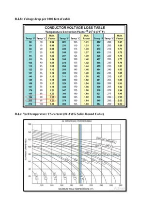
From the chart the voltage drop through cable is identified in the table below, those values
were taken for a temperature of 77°F,so a simple multiplication by a correction factor must be
done to take into account this difference (Appendix B.4.b).[3][8]
The table below shows the temperature correction factor estimation.
Table III- 12: Temperature correction factor estimation
Well name Cherouq1 Shaheen1 Badr6
Bottom-hole
temperature (°F)
197 198 195.8
Temperature
Correction Factor
1.27 1.26 1.25
B)Cable length
The total cable length should be at least 100ft (30m) longer than the measured pump
setting depth in order to make surface connections at safe distance from the wellhead.
To avoid the possibility of low voltage starts the cable length shall not exceed a maximum
value in order to skip a high cable voltage drop.[8]
The length of cable is the sum of the pump setting depth and at least additive safety length
equal to 100 feet.

63. 54
𝑉𝑜𝑙𝑡𝑎𝑔𝑒 𝐷𝑟𝑜𝑝 = 𝐿𝑖𝑛𝑒 𝐿𝑜𝑠𝑠𝑒𝑠 × 𝑇𝑒𝑚𝑝𝑒𝑟𝑎𝑡𝑢𝑟𝑒 𝐶𝑜𝑟𝑟𝑒𝑐𝑡𝑖𝑜𝑛 𝐹𝑎𝑐𝑡𝑜𝑟 III.36
The table below shows the voltage drop per 1000 feet calculation.
Table III- 13: Voltage drop per 1000 ft calculation
Well name Cherouq1 Shaheen1 Badr6
Line Losses
(Volt/1000)
43.33 43.33 43.33
Temperature
Correction Factor
1.27 1.26 1.25
Voltage
Drop(Volt/1000)
55.029 54.595 54.163
If we assume a surface cable length to of 100 ft.
𝑇𝑜𝑡𝑎𝑙 𝑉𝑜𝑙𝑡𝑎𝑔𝑒 𝐷𝑟𝑜𝑝 =
(𝑣𝑜𝑙𝑡𝑎𝑔𝑒 𝑑𝑟𝑜𝑝)×𝑙𝑒𝑛𝑔𝑡ℎ 𝑜𝑓 𝑐𝑎𝑏𝑙𝑒
1000
III.36
where 𝑙𝑒𝑛𝑔𝑡ℎ 𝑜𝑓 𝑐𝑎𝑏𝑙𝑒 = 𝑃𝑢𝑚𝑝 𝑆𝑒𝑡𝑡𝑖𝑛𝑔 𝐷𝑒𝑝𝑡ℎ + 𝑆𝑢𝑟𝑓𝑎𝑐𝑒 𝐶𝑎𝑏𝑙𝑒 III.37
The table below shows the total voltage drop calculation.
Table III- 14: Total voltage drop calculation
Well name Cherouq1 Shaheen1 Badr6
Pump Setting
Depth(ft)
10170.48 10170.48 10170.48
Surface Cable
length(ft)
100 100 100
Total Cable
Length(ft)
10270.48 10270.48 10270.48
Voltage
Drop(Volt/1000)
55.029 54.595 54.163
Total Voltage
Drop(Volt)
565.175 560.717 556.28
At the selected motor amperage and given down-hole temperature, the selection of a cable
size that will give a voltage drop of less than 30 volts per 1,000 ft. is usually recommended to
insure current carrying capability of cable.[3][8]
If the voltage drop is too low the starting torque may result in shaft breakage. Consider
using a VSD if the nameplate voltage drop is less than 5% (see equation III.38 in the next
page).[3][8]

64. 55
Applying these rules while selection:
 Total Voltage Drop/1000 ft < 30 V/1000 ft (better selection).
 Nameplate Voltage Drop
𝑁𝑎𝑚𝑒𝑝𝑙𝑎𝑡𝑒 𝑉𝑜𝑙𝑡𝑎𝑔𝑒 𝐷𝑟𝑜𝑝 =
𝑇𝑜𝑡𝑎𝑙 𝑉𝑜𝑙𝑡𝑎𝑔𝑒 𝐷𝑟𝑜𝑝
𝑀𝑜𝑡𝑜𝑟 𝑉𝑜𝑙𝑡𝑎𝑔𝑒
III.38
The table below shows the Motor nameplate voltage drop calculation.
Table III- 15: Motor nameplate voltage drop calculation
Well name Cherouq1 Shaheen1 Badr6
Total Voltage
Drop(V)
565.175 560.717 556.28
Motor Voltage(V) 2758 2066 2758
Nameplate Voltage
Drop
20.05 % 27.14 % 20.17 %
#4 AWG conductor is used in our case.
C) Conductor Temperature:
Selection of cable type is primarily based on fluid conditions and operating temperature.
The operating temperature can be determined using (Appendix B.4.c) based on the motor
current and the bottom-hole temperature.[3][8]
The table below shows the operating temperature of the power cable estimated.
Table III- 16: Power cable's operating temperature.
Well name Cherouq1 Shaheen1 Badr6
Bottom-hole
temperature (°F)
197 198 195.8
Current(am)
77 77 77
Conductor
temperature(°F)
260 263 257
All conductor temperatures are below 280°F that's why we choose CENR (Copper Conductor,
EPDM insulation, Nitrile jacket, Both round or flat, armor galvanized) to withstand
temperature requirements (Appendix B.4.d).
D) Insulation KV choice:
Based on the surface voltage requirements, the insulation type is chosen:[3][8]
𝑆𝑢𝑟𝑓𝑎𝑐𝑒 𝑉𝑜𝑙𝑡𝑎𝑔𝑒 = 𝑀𝑜𝑡𝑜𝑟 𝑉𝑜𝑙𝑡𝑎𝑔𝑒 + 𝑉𝑜𝑙𝑡𝑎𝑔𝑒 𝐷𝑟𝑜𝑝 III.39

65. 56
The table below shows the surface voltage calculation
Table III- 17: Surface Voltage calculation
Well name Cherouq1 Shaheen1 Badr6
Total voltage drop
(Volt)
565.175 560.717 556.28
Motor voltage(Volt) 2758 2066 2758
Surface
voltage(Volt)
3323.175 2626.717 3314.28
Baker Hughes manufacturer gives 3KV, 4KV, 5KV options for insulation voltage classified
into 2 artificial lift series [9]:
- Superior Performance (SP) series for sandy wells.
- Extreme Performance (XP) series for corrosive wells.
In our case the SP series is chosen because it provides abrasion protection. Mind that the
surface voltage is above 3KV we should select through 4KV or 5KV option. Our choice is
5KV insulation voltage for more security.
CENR: EPDM (C76243) round cable is our choice for the three wells. Round options is the
suited shape, we will select the round configuration under the reference: CENR (C76243)
with nominal dimension of 1.18. (Appendix B.4.e)
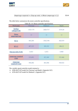
III.1.1.9. Motor controller selection
Our choice is based on two features identifying a transformer or a motor controller which are
voltage and amperage required:[9]
A) voltage
We determine the KVA required for the transformer:
𝐾𝑉𝐴 = (
𝑆𝑢𝑟𝑓𝑎𝑐𝑒 𝑉𝑜𝑙𝑡𝑎𝑔𝑒 × 𝑀𝑜𝑡𝑜𝑟 𝐴𝑚𝑝𝑒𝑟𝑎𝑔𝑒 × √3
1000
)
III.40
We must consider a safety margin of 10% by multiplying the value of KVA by 1.1 in order to
withstand unexpected fluctuations.
𝐾𝑉𝐴 ∗= (
𝑆𝑢𝑟𝑓𝑎𝑐𝑒 𝑉𝑜𝑙𝑡𝑎𝑔𝑒 × 𝑀𝑜𝑡𝑜𝑟 𝐴𝑚𝑝𝑒𝑟𝑎𝑔𝑒 × √3
1000
) × 1.1 III.41
B) Amperage:
 Determine step up ratio
𝑆𝑡𝑒𝑝 𝑢𝑝 𝑟𝑎𝑡𝑖𝑜 = (
𝑠𝑢𝑟𝑓𝑎𝑐𝑒 𝑣𝑜𝑙𝑡𝑎𝑔𝑒
480
) III.42
 Multiply step up ratio by motor amperage
𝐴𝑚𝑝𝑒𝑟𝑎𝑔𝑒 𝑟𝑒𝑞𝑢𝑖𝑟𝑒𝑑 = 𝑆𝑡𝑒𝑝 𝑢𝑝 𝑟𝑎𝑡𝑖𝑜 × 𝑀𝑜𝑡𝑜𝑟 𝑎𝑚𝑝𝑒𝑟𝑎𝑔𝑒 III.43
We must consider a safety margin of 10% by multiplying the value of Amperage required by
1.1 in order to withstand unexpected fluctuations.

66. 57
𝐴𝑚𝑝𝑒𝑟𝑎𝑔𝑒 𝑟𝑒𝑞𝑢𝑖𝑟𝑒𝑑 ∗= 𝑆𝑡𝑒𝑝 𝑢𝑝 𝑟𝑎𝑡𝑖𝑜 × 𝑀𝑜𝑡𝑜𝑟 𝑎𝑚𝑝𝑒𝑟𝑎𝑔𝑒 × 1.1 III.44
The table below summarizes the motor controller specifications.
Table III- 18: Motor controller specifications
Well name Cherouq1 Shaheen1 Badr6
Surface
voltage(Volt)
3323.175 2626.717 3314.28
Motor
amperage(Am)
77 77 77
KVA 443,205 350,3198 442.019
KVA* 487,525 385,352 486.22
Step up ratio (Volt) 6,923 5,472 6.905
Amperage required
(Am)
533,093 421,369 531.666
Amperage
required*(Am)
586,402 463,506 584.832
The variable speed controller model retained is:
 4500-4GCS 6P model for Cherouq1 and Badr6. (Appendix B.5)
 4350-4GCS 6P model for Shaheen1. (Appendix B.5)

67. 58
Table III- 19: ESP design summary (Cherouq1)
Production
requirement
3000 bpd
Manufacturer
Supervisor Mr. Mohamed Ali Khyari (OMV Production engineer)
Design engineer Omar Omrane (Petroleum engineer)
Company OMV
Pump
Series 538 Model P37 Build SSD
Stages 189
Rate @
best
efficiency
520 M3
/D ( ≈3270 bpd )
Gas separator Not required
Motor
Series 450 Model SP
Voltage 2758 V Amperage 77 Am
Horse
Power
334 Hp
Seal section Series 513 Model GSB3
Electric cable
Conductor 4# AWG Insulation EPDM
Insulation
Voltage
5KV
Material
N°
CENR
(C76243)
Shape Round Diameter 1.18 in
Armor Galvanized
Variable Speed
Controller
Model
4500-
4GCS 6P
KVA* 519 Amperage 624 Am

68. 59
Table III- 20: ESP design summary (Shaheen1)
Production
requirement
1623 bpd
Manufacturer
Supervisor Mr. Mohamed Ali Khyari (OMV Production engineer)
Design engineer Omar Omrane (Petroleum engineer)
Company OMV
Pump
Series 538 Model P23 Build SSD
Stages 234
Rate @
best
efficiency
320 M3
/D ( ≈2013 bpd )
Gas separator GSR538 (95 % efficiency)
Motor
Series 450 Model SP
Voltage 2066 V Amperage 77 Am
Horse
Power
250 Hp
Seal section Series 513 Model GSB3
Electric cable
Conductor 4# AWG Insulation EPDM
Insulation
Voltage
5KV
Material
N°
CENR
(C76243)
Shape Round Diameter 1.18 in
Armor Galvanized
Variable Speed
Controller
Model
4350-
4GCS 6P
KVA* 390 Amperage 369 Am

69. 60
Table III- 21: ESP design summary(Badr6)
Production
requirement
1660 bpd
Manufacturer
Supervisor Mr. Mohamed Ali Khyari (OMV Production engineer)
Design engineer Omar Omrane (Petroleum engineer)
Company OMV
Pump
Series 538 Model G31 Build SXD
Stages 192
Rate @
best
efficiency
420 M3
/D ( ≈2641 bpd )
Gas separator GSR538 (95 % efficiency)
Motor
Series 450 Model SP
Voltage 2758 V Amperage 77
Horse
Power
334 Hp
Seal section Series 513 Model FSFB3
Electric cable
Conductor 4# AWG Insulation EPDM
Insulation
Voltage
5KV
Material
N°
CENR
(C76243)
Shape Round Diameter 1.18 in
Armor Galvanized
Variable Speed
Controller
Model
2250-
4GCS 6P
KVA* 519 Amperage 624 Am
III.2. Software design
III.2.1. AutographPC brief overview
Centrilift application engineers use AutographPC to size, simulate and optimize the best
solution for all types of well conditions. The simulator is a powerful feature that models pump
operating conditions and greatly aids in troubleshooting. Since 1986 AutographPC has been
continually updated and enhanced by a dedicated group of Centrilift engineers and

70. 61
programmers. AutographPC is unique in the industry in that it is the only software developed
and maintained by an ESP system manufacturer.
III.2.2. AutographPC purpose
This software aims to perform calculations based on entered well data, select the best
equipment for the application by testing the suitability of specific conditions and perform the
hand sizing done as a first step.
III.2.3. AutographPC features
Perhaps the most important feature of AutographPC is the internal database built on over a
half-century of Centrilift engineering and development experience. The interactive, on-line
technical assistance is similar to having direct access to the Centrilift engineering department
with decades of experience is sizing and development of electrical submersible pumping
systems.
AutographPC is the tool that integrates the Centrilift system components. Each component
is an integral part of the system and possesses characteristics and efficiencies not found in the
products of other manufacturers.
III.2.4. AutographPC modeling Application (Cherouq 1 well)
III.2.4.1. Problematic and Purpose
In this paragraph we will try to optimize Cherouq1 well production by choosing the fitting
ESP system components for this well. As the company had already in stock many components
previously installed in other wells such as (Ameni1, Ameni2, Nada1 and Maha1) we will try
to choose some among these components. After testing the four available pumps
(P31,P17,P11,G31) corresponding respectively to (Ameni1, Ameni2, Nada1, Maha1) we
conclude that the best one fitting Cherouq is P31 pump with more stages required than
existing. For this reason we will base all our sizing on this choice with the minimum
modification of the other components. The following paragraphs will detail the approach of
our study.
III.2.4.2. Data required for design
The table below assembles the well input data required for software design.
Table III- 22: Well input Data (Software Design)
Fluid Properties
Oil Specific Gravity 42.3 °API
Water cut 89.5 %
Specific Gravity of Water 1.2 Relative to H2O
Specific Gravity of gas 0.84 Relative to air
Producing GOR 1577 Scf/STB
Bubble point pressure 4800 Psia
Temperature Model
Fluid Surface Temperature
(WHT)
109 °F
Earth surface temperature (65)Estimated by software °F
Bottom Hole Temperature 197 °F
Gas impurities
Percentage of N2 0 %

71. 62
Percentage of H2S 0 %
Percentage of CO2 0 %
Inflow performance-Test data
Datum Measured Depth 11164 Ft
Perforations Measured Depth 11164 Ft
Static pressure(Pr) 4200 Psi
PI @ zero flow 1.8 BPD/psi
String Description (Well Profile)
Total Vertical Depth
From 0 to 6194 ft (cased with
8.681" Casing ID)
Ft
Total Vertical Depth
From 6194 to 11164 ft (cased
with 6.094" Casing ID)
Ft
Target
Pump Depth 10170 Ft
Flowrate max 3000 Bpd
Minimum Pump Intake
Pressure
2041(estimated by software) psi
Gas separator efficiency (95%)
IPR method (Vogel Composite)
Surface Pressures
Tubing pressure 200 Psi
Casing pressure 100 Psi
The well Conditions Screen (or well screen) is opened by selecting the tab marked 'Well.' The
well screen allows the input of values fundamental to the application being sized.
AutographPC uses data entered into the well screen to complete all the following aspect of the
application. It is absolutely crucial the information entered into the well s accurate and
current.
Figure III- 6: well conditions screen capture

72. 63
Figure III-6 is a screen capture of the AutographPC Well Conditions Screen. After filling the
blank fields with the required input Well data it remains just to compute in order to arrive at
the total dynamic head value using some intermediate data (see FigureIV-6).
The compute section is divided into several sub-sections including:
 Inflow Performance
 Intake Conditions
 Discharge Conditions
The table below represents the output well data.
Table III- 23: Well Output Data (Software Design)
Inflow Performance
Perforations pressure(Pperfs)
(Static)
4200 Psi
Productivity Index PI 1.8 BPD/psi
Theoretical maximum flowrate
(MaxQ/AOF)
7219 BPD
Perforations pressure(Pperfs)
(flowing/Dynamic)
2505 Psi
Intake conditions
PIP(Pump Intake Pressure) 2041 Psi
Qipbs (Flowrate before
separation)
3500 BPD
GIPbs (% gas (free gas) into the
pump before separation)
8.579 %
QIP(Flowrate at pump intake) 3215 BPD
GIP(% gas into the pump (after
separation)
0.467 %
GORpump (gas oil ratio at pump
depth)
761.2 Scf/STB
Bo 1.413 -
Bg 1.295 -
Bw 1.032 -
FLOP(fluid level over the pump) 4060 Ft
ViscLiq(Liquid viscosity) 0.658 Cp
Discharge conditions
Pdp(Pump discharge pressure) 5095 Psi
Qdp (Flowrate at pump
discharge)
3240 BPD
Bo(oil formation volume factor) 1.378 -
Bg(oil formation volume factor) 0.638 -
Bw(water formation volume
factor)
1.026 -
SGmix(Mixture (oil, water &
gas) specific gravity)
1.126 rel-H2O -
ViscLiq(Liquid viscosity) 0.778 Cp
%H2O(Water cut as measured at
the surface)
91.04 %
TDH(Total Dynamic Head 1940 M

73. 64
III.2.4.3. Pump sizing screen
Figure III- 7: Pump sizing screen capture
The pump screen allows the user to select from a wide inventory of possible solutions to find
the most appropriate pump for the application. In this section we conserve the current
available pump of Ameni1 well by increasing the number of stages from 34 stages to 129
stages (FigureIII-7) because the total dynamic head of Cherouq 1 is higher than that refers to
Ameni1.
The table below shows the pump specifications.
Table III- 24: Pump sizing specifications (Software Design)
Series & model: 538/P31/CENTURION
Intake pumping conditions
Pressure 2005 Psi
Flowrate 3281 BPD/day
Specific Gravity 1.113 -
Viscosity 0.657 Cp
Discharge pumping conditions
Pressure 5095 Psi
Flow rate 3240 BPD/day
Specific Gravity 1.126 -
Viscosity 0.778 Cp
Design point
Number of stages 129 -
Flow rate at the surface 3064 BPD
TDH(Total Dynamic Head) 1940 m
BHP(Brake Horse Power) 267.1 Hp
Frequency 59.7 Hz

74. 65
III.2.4.4. Motor sizing screen
Figure III- 8: Motor sizing screen capture
The motor screen contains three data entry fields. They are:
 Input data
 ADR( Application dependent rating)
 Selection(60Hz rating)
In This section we modified just the "selection(60Hz rating)" option by changing the motor
from 450MSP to 450MSP1 to guarantee the horse power required to operate the new pump
and the seal.(Figure III-8)
Table III- 25: Motor sizing specifications (Software Design)
Selection(60Hz rating)
Manufacturer CENTRILIFT -
Series & model 450MSP1. -
Oil type CL5 -
Hose power 300 Hp
Voltage 3510 Volt
Amperage 55 Am
Number of rotors 30 -
Operating Conditions (59.7 Hz )
Motor load 89.83 %
Voltage 3410 V
Amperage 50.41 Am
Internal temperature 256.9 °F
Efficiency 84.74 %
Shaft Speed 3419 RPM

75. 66
III.2.4.5. Seal sizing screen
Figure III- 9: Seal sizing screen capture
The seal screen (Figure III-9) contains two data entry fields:
 Application - related data
 Seal selection
This is the only screen that cannot be used independently of all other screens. Both pump and
motor must be chosen before a seal can be selected.
This section remains the same for Ameni1 well that means we conserved also the same seal of
Ameni1 well.
The table below contains the main parameters of our seal:
Table III- 26: Seal sizing specifications (Software Design)
Seal Selection
Brand CENTRILIFT -
Series 513 -
Model GSB3 -
III.2.4.6. Cable sizing screen
Figure III- 10: Cable sizing screen capture

76. 67
The cable sizing screen (Figure III-10) can be used by itself or as part of a complete system
sizing. As the seal section the cable remain the same for Cherouq1 well. Thus the company
will not buy a new one for this ESP installation.
The screen is divided into four main sections:
 Cable input data
 Cable selection
 Cable sizing output
The table below summarizes the major parameters of the cable chosen.
Table III- 27: Cable sizing specifications (Software Design)
Cable selection
Brand Centrilift -
Type #4 CELR 5KV -
Cable sizing output
Voltage Drop 291.9 V
Power loss 25.2 KW
III.2.4.7. Controller sizing screen
Figure III- 11: controller sizing screen capture
The controller sizing screen (Figure IV-11) can be used by itself or as part of a complete
system sizing.
In this section we changed the controller of Ameni1 well by a new one 8600-VT to better
work with the new motor for Cherouq1 well.
The screen is divided into four main sections:
 input data
 Controller selection
 Transformer
 Controller sizing screen

77. 68
The table below summarizes the major parameters of the cable chosen
Table III- 28: Controller sizing specifications (Software Design)
Selected equipment
Model 8600 VT -
KVA 494 -
Amps 750 Am
III.3. Conclusion
In this chapter we intended to present the electrical submersible pump design procedure by
both methods: 9 steps hand sizing design and AutographPC design. The main objective was to
apply these two methods on specific wells of Anaguid field.

78. 69
Chapter IV: Economic Study
Objective
This chapter aims to estimate the profitability
of the project by calculating the net cashflow
and knowing the payback period.

79. 70
Development of oil and gas accumulation is a high cost venture. Therefore any project
must promise sufficient return on the money absorbed to at least pay the interest on loans and
pay the dividend expected by the shareholders. The economic model for evaluation of
investment opportunities is normally constructed as Excel spreadsheet using the techniques to
be produced in this section.
The project cashflow is the forecast of the money absorbed and the money generated
during the project lifetime. Initially the cashflow will be dominated by the CAPEX required to
construct the equipment for the project (e.g. platform, pipeline, wells, and compression
facilities). Once production commences revenues are used to recover the CAPEX of the
project to pay for the OPEX of the project(e.g. manpower, maintenance, equipment running
costs, support costs) and to provide the host government take.
IV.1. Project net cashflow
Most projects are expected to grant cash flows over a period of time.
𝑷𝒓𝒐𝒋𝒆𝒄𝒕 𝒏𝒆𝒕 𝒄𝒂𝒔𝒉 𝒇𝒍𝒐𝒘 = 𝒓𝒆𝒗𝒆𝒏𝒖𝒆𝒔 − 𝑪𝑨𝑷𝑬𝑿 − 𝑶𝑷𝑬𝑿 − 𝑹𝑶𝒀𝑨𝑳𝑻𝒀 IV.46
 Revenue items
In most cases the revenues will be due to the sale of hydrocarbons. In determining these gross
revenues, oil and gas prices must be assumed following the current worldwide value.
𝒎𝒐𝒏𝒕𝒉𝒍𝒚 𝒓𝒆𝒗𝒆𝒏𝒖𝒆𝒔 = (𝒑𝒓𝒐𝒅𝒖𝒄𝒕𝒊𝒐𝒏/𝒅𝒂𝒚) × 𝒐𝒊𝒍 𝒑𝒓𝒊𝒄𝒆 × 𝒏𝒖𝒎𝒃𝒆𝒓 𝒐𝒇 𝒅𝒂𝒚𝒔 IV.47
 Expenditure items(CAPEX and OPEX)
These expenditures are handled by the fiscal system established by the host government. They
are typically defined as CAPEX such as costs of platforms pipelines wells items whose useful
life is less than year, as for chemicals services maintenances overheads insurance costs would
then be classed as OPEX.
The OPEX is estimated based on its two components: Fixed OPEX and Variable OPEX.
Fixed OPEX is proportional to the cost of the items to be operated therefore based on a
percentage of the cumulative CAPEX.
Variable OPEX is proportional to the production rate.
𝑫𝒂𝒚𝒍𝒚 𝑶𝑷𝑬𝑿 = Diesel consumption and trucking + generator maintenance and
catering
= 𝟓𝟎𝟎 + 𝟕𝟎𝟎 = 𝟏𝟐𝟎𝟎 $
IV.48
 Host government take
The most traditional fiscal system is the tax and royalty scheme.
Royalty is generally defined as a percentage of the total revenues from the sale of oil and gas.
𝑹𝒐𝒚𝒂𝒍𝒕𝒚 = 𝑹𝒐𝒚𝒂𝒍𝒕𝒚 𝒓𝒂𝒕𝒆(%) × 𝒑𝒓𝒐𝒅𝒖𝒄𝒕𝒊𝒐𝒏(𝒃𝒃𝒍) × 𝒐𝒊𝒍 𝒑𝒓𝒊𝒄𝒆($/𝒃𝒃𝒍)
𝑹𝒐𝒚𝒂𝒍𝒕𝒚 = 𝟎. 𝟏 × 𝒑𝒓𝒐𝒅𝒖𝒄𝒕𝒊𝒐𝒏(𝒃𝒃𝒍) × 𝒐𝒊𝒍 𝒑𝒓𝒊𝒄𝒆($/𝒃𝒃𝒍)
IV.49
 Internal rate of return (IRR)

80. 71
IRR is a parameter used to measure the profitability of investment. It is the discount rate that
makes the net present value (NPV) equal to zero
 Net present value (NPV)
Net Present Value NPV is the sum of all project cash flows, discounted back to a common
point in time.
 Expected Monetary Value (EMV)
Expected Monetary value is the total of the weighted outcomes (payoffs) associated with a
decision, the weights reflecting the probability of the alternative events that produce the
possible payoff. It is expressed mathematically as the product of an event's probability of
occurrence and the gain or loss that will result.
𝐸𝑀𝑉 = 𝑃𝑂𝑆 × 𝑁𝑃𝑉 − (1 − 𝑃𝑂𝑆) × 𝐶𝐴𝑃𝐸𝑋 IV.50
Where
POS: Probability Of Success
NPV: Net Present Value of all the period of investment
 Productivity decline factor
The productivity decline factor represents a percentage of production rate discount which is
assumed as 4% a month based on the history of previous produced wells of the same field.
 Payback period
Payback incorporates the idea of recovering one’s investment. In its simplest form, it is the
point at which the cumulative NCF returns to zero. The Payback “Period” is defined as the
time taken, from the start of the project, to reach this position.
IV.2. Excel results
Expected start: September 2016
CAPEX: 3,200,000$
OPEX: 1200 USD/day
Expected Total production after reactivation
= ESP production rate × (1 − Wc) IV.51
= 3064 × (1 − 0.895) = 321 bbl/day
Economic Limit: 100 STB/day
Assumptions:
Oil Prices: 40 USD/bbl
Discount rate r=10%
Probability of success: POS=80%
CAPEX:

81. 72
The table below contains the different terms of the CAPEX
Table IV- 1: CAPEX calculation
Description Unit Price($)
ESP package
ESP equipment 1 350,000
ESP Backup 1 200,00
ESP services 1 220,000
ESP Monitoring 1 100,000
VSD spare parts 1 30,000
Power Gen package + Construction & Civil Work
Diesel gensets 650 KVA 1 160,000
Two years spare parts 1 15,000
Gas gensets 600 KVA 1 850,000
Two years spare parts 1 25,000
Diesel tank 20 Cubic Meters 1 25,000
Diesel feet pump 1 25,000
MCC 1 80,000
Cables 1 15,000
Shelter extemal Lightning 1 35,000
Civil works 1 110,000
Mechanical & Electrical
works
1 135,000
Site supervisions & execution 1 25,000
Commissioning & start up 1 15,000
Workover Operations &
services
1 1,500,000
Total cost per well site = 3,915,000
Contingency per well site (10%) = 391,500
CAPEX= Total cost per well site + Contingency per well site = 4,306,500
The assumption of the total higher value of CAPEX possible is nearly 4300 M$ but when we
contacted services companies to order just what we need the final value of CAPEX turns into
3200 M$.
Net Cash Flow calculation
The table below shows the Net Cash Flow calculation of the project.
Table IV- 2: Net Cash Flow calculation
year month days
Prod
rate
Royalty OPEX NCF
Cum
NCF
CUM
OIL
bbl/d M $ M $ M $ M $ MMSTB
-
3200
2016 June
-16
30 322 38,6
36,00 311
-
2889 0,0097
July
-16
31 309 38,3
37,20 307
-
2581 0,0096
Augest -16 31 296 36,8
37,20 294
-
2287 0,0092
September 30 285 34,2 36,00 271 - 0,0085

82. 73
-16 2016
October -
16
31 273 33,9
37,20 268
-
1748 0,0085
November
-16
30 262 31,5
36,00 247
-
1501 0,0079
December
-16
31 252 31,2
37,20 244
-
1257 0,0078
2017
January -
17
31 242 30,0
37,20 233
-
1024 0,0075
February -
17
28 232 26,0
33,60 200 -824 0,0065
March
-17
31 223 27,6
37,20 211 -613 0,0069
April
-17
30 214 25,7
36,00 195 -418 0,0064
May
-17
31 205 25,5
37,20 192 -226 0,0064
June
-17
30 197 23,7
36,00 177 -49 0,0059
July
-17
31 189 23,5
37,20 174 125 0,0059
Augest -17 31 182 22,5 37,20 166 291 0,0056
September
-17
30 174 20,9
36,00 152 443 0,0052
October -
17
31 167 20,8
37,20 150 593 0,0052
November
-17
30 161 19,3
36,00 138 730 0,0048
December
-17
31 154 19,1
37,20 135 865 0,0048
2018
January -
18
31 148 18,4
37,20 128 993 0,0046
February -
18
28 142 15,9
33,60 110 1103 0,0040
March
-18
31 137 16,9
37,20 115 1218 0,0042
April
-18
30 131 15,7
36,00 106 1324 0,0039
May
-18
31 126 15,6
37,20 103 1427 0,0039
June
-18
30 121 14,5
36,00 94 1521 0,0036
July
-18
31 116 14,4
37,20 92 1614 0,0036
August
-18
31 111 13,8
37,20 87 1701 0,0035
September
-18
30 107 12,8
36,00 79 1780 0,0032
October -
18
31 103 12,7
37,20 77 1857 0,0032

83. 74
NVP calculation
𝑁𝑃𝑉 = − 𝐶𝐴𝑃𝐸𝑋 + ∑
𝑁𝐶𝐹𝑛
(1 + 𝑟) 𝑛/12
𝑀
𝑛=1
= 1409 𝑀$ IV.52
Where
n: month
M: number of months
NCFn: Net Cashflow for n month
r: discount rate = 10%
EMV calculation
As said the possibility of the success of the project is 80%, So
𝐸𝑀𝑉 = 80%(𝑁𝑃𝑉) − 20%(𝐶𝐴𝑃𝐸𝑋) = (
80 × 1409
100
) − (
20 × 3200
100
) = 487 > 0 IV.52
A positive value here signifies a benefit.
Figure IV-1 and Figure IV-2 are respectively the production decline profile and the Cashflow
profile.
Figure IV- 1: Production decline profile
Figure IV- 2: Cashflow profile
IV.3. Interpretation
A positive Net Present Value NPV indicates that the project earnings generated exceeded
the anticipated costs and possible losses.
The very high internal rate of return reveals a continuously lucrative quality about
installing an ESP for the studied well. It shows that this affair is treated in a very cost
effective way.

84. 75
The payback period is equal to 14 months when the cumulative Net Cashflow becomes
positive.
IV.4. Conclusion
As a highly safe and rentable project, this venture seems to grant covering the expenditures
and warrant great amount of returns to encourage the company start investing in it.

85. 76
General conclusion
This report has focused on the ESP design for 3 wells (Cherouq1, Shaheen1 and Badr6) of
Anaguid Oil Field.
The ESP artificial lift selection is legitimized by the company's strategy based on technical
and economical evaluation.
Although the Nine Steps Hand Sizing method and the AutographPC software provided
almost similar ESP design and tiny gaps, a comparative analysis reveals the following
remarks;
In one hand, the hand sizing is built upon theoretical studies and complicated equations,
which requires a considerable knowledge of field and oil and gas notions which is deeply
interesting for production engineers.
However the selection of ESP equipment based on manual charts takes long time and gives
imprecise results. Moreover, the updating operation of database is quite hard.
In the other hand, the AutographPC is friendly user software, with a wide updated database
and advanced digital calculations but it is more oriented for ESP constructors; it lacks of some
petroleum and reservoir notions and understanding.
Therefore, combining both design methods can provide an effective ESP selection.

86. References
[1] HERIOT WATT UNIVERSITY, PRODUCTION TECHNOLOGY I, ,PRODUCTION
DEPARTMENT, 2010
[2] HERIOT WATT UNIVERSITY, PRODUCTION TECHNOLOGY II, PRODUCTION
DEPARTMENT, 2010
[3] BAKER HUGHES CENTRILIFT, SUBMERSIBLE PUMP HAND BOOK NINTH EDITION,
PRODUCTION DEPARTMENT, 2009
[4] SHLUMBERGER, ARIFICIAL LIFT SYSTEMS, PRODUCTION DEPARTMENT, 2008
[5] GABOR TAKACS, ELECTRICAL SUBMERSIBLE PUMP MANUAL: OPERATIONS,
TECHNOLOGY AND MAINTENANCE, PRODUCTION DEPARTMENT, 2009
[6] BAKER HUGHES CENTRILIFT, CENTRILIFT PUMP CURVES, PRODUCTION DEPARTMENT,
2007
[7] GABOR TAKACS, DESIGN AND ANALYSIS OF ESO INSTALLATIONS, PRODUCTION
DEPARTMENT, 2009
[8] BAKER HUGHES CENTRILIFT, CENTRILIFT NINE STEPS FOR ESP DESIGN, PRODUCTION
DEPARTMENT, 2005
[9] BAKER HUGHES CENTRILIFT, BAKER HUGHES ESP TECHNICAL REFERENCE,
PRODUCTION DEPARTMENT, 2011

87. Appendices
Appendix A: Fluid properties calculations
 A.1. Moody diagram: Friction factor
 A.2. Pseudo-Critical TEMPERATURE and PRESSURE diagram
 A.3. Compressibility factor
Appendix B: ESP design
 B.1. Pump selection
 B.2. Motor selection
 B.3. Seal Section selection
 B.4. Power Cable selection
 B.5. Motor Controller selection
Appendix C: Conversion Table

88. Appendix A: Fluid properties calculation
A.1.a. : Moody diagram: Friction factor (From the bottom-hole to the pump friction
calculation)

89. A.1.b. : Moody diagram: Friction factor (From the Static level of the fluid to the surface
friction calculation)

90. A.2: Pseudo-Critical TEMPERATURE and PRESSURE diagram

91. A.3: Compressibility factor

92. Appendix B: ESP design
B.1. ESP selection[6]
B.1.a: Performance Series 538P37 Pump[6]

93. B.1.b: Performance Series 538P23 Pump[6]
B.1.c: Performance Series 538G31 Pump[6]

94. B.2.a: 513&538 Series Seal sections[6]
B.2.b: 400 Series Seal sections[6]

95. B.3.a: 450 SP 200°F Motors.[6]
B.4.a: Voltage drop per 1000 feet of cable

96. B.4.b: Voltage drop per 1000 feet of cable
B.4.c: Well temperature VS current (#4 AWG Solid, Round Cable)

97. B.4.d: Voltage drop per 1000 feet of cable
B.4.e: SP cable performance
B.5: Motor Controller selection

98. C: Table of Conversion