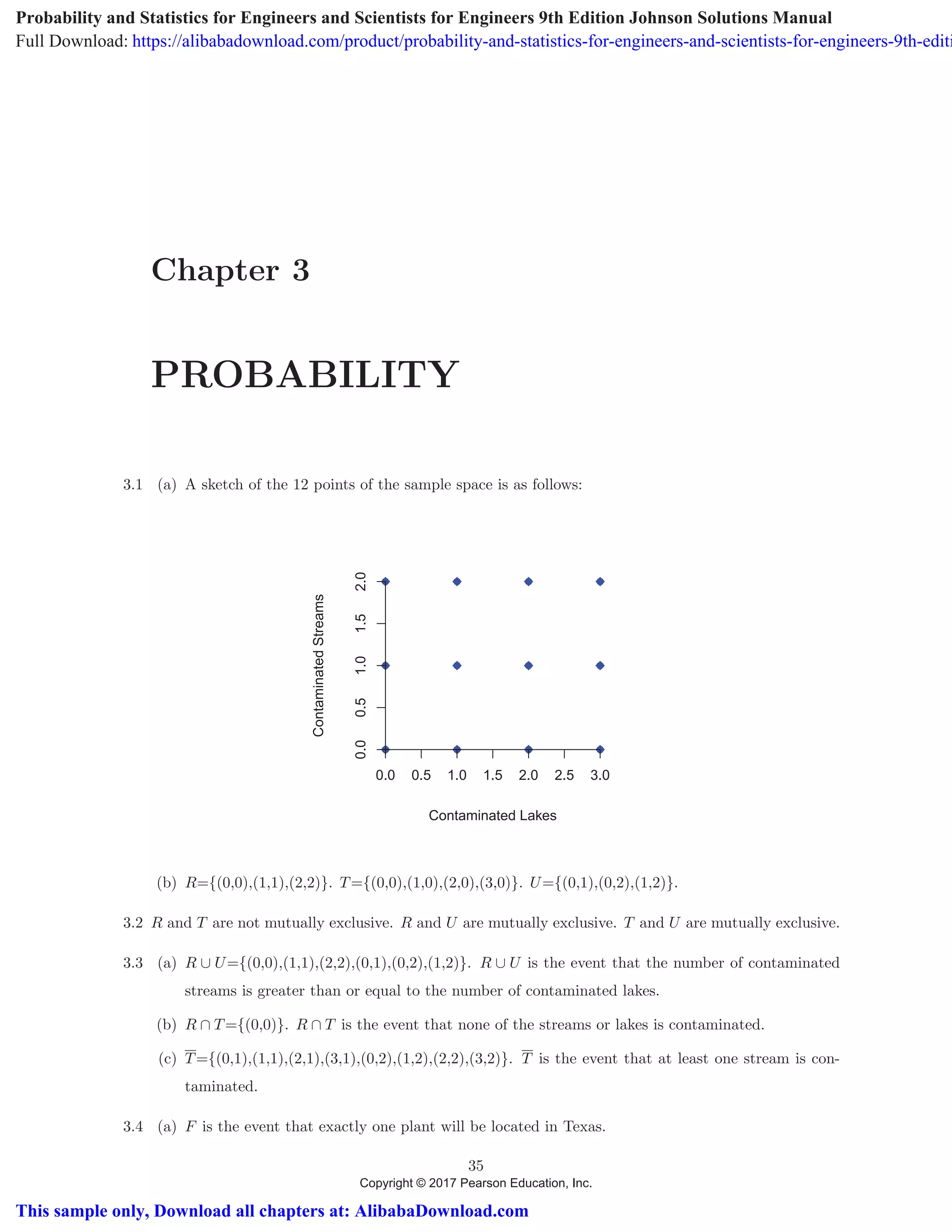
The document discusses various concepts in probability including sample spaces, mutually exclusive events, unions and intersections of events, permutations, combinations, and the use of Venn diagrams. It covers probabilities related to specific scenarios, outlining calculations for selecting elements and determining possible outcomes. The chapter also introduces tree diagrams and provides example problems with their solutions.

![40 CHAPTER 3 PROBABILITY
3.24 There are
12C4 =
⎛
⎝
12
4
⎞
⎠ =
12!
4! 8!
= 495 ways
to select the 4 candidates to interview.
3.25 There are 12C3 = 220 ways to draw the three rechargeable batteries.
There are 11C3 = 165 ways to draw none are defective.
(a) The number of ways to get the one that is defective is 220 − 165 = 55.
(b) There are 165 ways not to get the one that is defective.
3.26 (a) There are 10C3 = 120 ways to get no defective batteries.
(b) There are 2 · 10C2 = 90 ways to get 1 defective battery.
(c) There are 10C1 = 10 ways to get both defective batteries.
3.27 There are 8C2 ways to choose the electric motors and 5C2 ways to choose the switches. Thus, there
are
8C2 · 5C2 = 28 · 10 = 280
ways to choose the motors and switches for the experiment.
3.28 (a) Using the long run relative frequency approximation to probability, we estimate the probability
of a required warranty repair by
P [ Warranty repair required ] =
72
880
= 0.0818
The number of trials 880 is quite large so the relative frequency should be close to the probability.
(b) Using the data from last year, the long run relative frequency approximation to probability gives
the estimate
P [ Receive season ticket ] =
6000
8400
= 0.714
One factor is the expected quality of the team next year. If the team is expected to be much
better next year more students will apply for tickets.
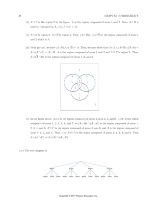
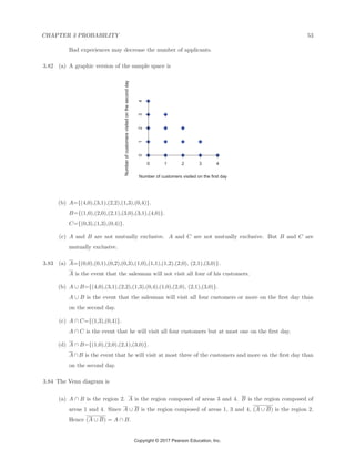
3.29 The outcome space is given in Figure 3.1.
(a) The 6 outcomes summing to 7 are marked by squares. Thus, the probability is 6/36 = 1/6.
(b) There are 2 outcomes summing to 11, which are marked by diamonds. Thus, the probability is
2/36 = 1/18.
(c) These events are mutually exclusive. Thus, the probability is 6/36 + 2/36 = 2/9.
Copyright © 2017 Pearson Education, Inc.](https://image.slidesharecdn.com/probability-and-statistics-for-engineers-and-scientists-for-engineers-9th-edition-johnson-solutions--200101130110/85/New-Perspectives-on-HTML5-CSS3-JavaScript-6th-Edition-Carey-Solutions-Manual-6-320.jpg)
![46 CHAPTER 3 PROBABILITY
But 1/3 + 1/4 = 7/12 > 1/2 which is a contradiction.
3.55 P(I ∩ D) = 10/500, P(D) = 15/500, P(I ∩ D) = 20/500, P(D) = 485/500.
P(I|D) =
P(I ∩ D)
P(D)
=
10
15
=
2
3
,
P(I|D) =
P(I ∩ D)
P(D)
=
20
485
=
4
97
.
3.56 (a) The probability of major repairs would increase. High mileage causes many major parts to wear
out.
(b) The probability of knowing the second law of thermo-
dynamics would increase. The typical college senior would not know the law but most mechanical
engineers would learn the laws of thermodynamics.
(c) Let A = [ major repairs required ] and B = [ high mileage ]. The question concerns the relation
of the conditional probability P( A | B ) to the unconditional probability P( A ).
3.57 (a) The sample space is C. Thus the probability is given by:
N(A ∩ C)
N(C)
=
8 + 15
8 + 54 + 9 + 14
=
62
85
= .73.
(b) This is given by:
N(A ∩ B)
N(A)
=
20 + 54
20 + 54 + 8 + 2
=
74
84
= .881.
(c) This is given by:
N(C ∩ B)
N(B)
=
N((C ∪ B))
N(B)
=
150 − 121
105 − 99
=
29
51
= .569.
3.58 (a)
P(A|B) =
P(A ∩ B)
P(B)
=
.06 + .04
.06 + .04 + .19 + .11
= .25.
(b)
P(B|C) =
P(B ∩ C)
P(C)
=
.19 + .06
1 − .4
= .417.
(c)
P(A ∩ B|C) =
P(A ∩ B ∩ C)
P(C)
=
.04
.4
= .1.
(d)
P(B ∪ C|A) =
P((B ∪ C) ∩ A)
P(A)
=
.09 + .11. + .19
1 − .5
= .78.
(e)
P(A|B ∪ C) =
P(A ∩ (B ∪ C))
P(B ∪ C)
=
.06 + .04 + .16
.06 + .04 + .16 + .19 + .11 + .09
=
.26
.65
= .4
Copyright © 2017 Pearson Education, Inc.](https://image.slidesharecdn.com/probability-and-statistics-for-engineers-and-scientists-for-engineers-9th-edition-johnson-solutions--200101130110/85/New-Perspectives-on-HTML5-CSS3-JavaScript-6th-Edition-Carey-Solutions-Manual-12-320.jpg)
![52 CHAPTER 3 PROBABILITY
=
.7 × .1
.7 × .1 + .2 × .9
=
.07
.07 + .18
= .28
(b)
P(C|A) =
P(A|C)P(C)
P(A|C)P(C) + P(A|C)P(C)
=
(1 − .7) × .1
(1 − .7) × .1 + (1 − .2) × .9
=
.03
.03 + .72
= .04
3.80 Let A be the event that a circuit board passes the automated test and D be the event that the board
is defective. We approximate P(A|D) = 25/30 and P(A) = 890/900
(a) We then approximate P( Pass test | board has defects ) = P(A | D) using the relation
25
30
= P(A | D) = 1 − P(A | D)
or P(A | D) = 5/30.
(b) The approximation P(A | D) = 5/30 may be too small because the boards were intentionally made
to have noticeable defects. Likely, many defects are not very noticeable.
(c) To proceed, we assume that P(A | D) = 0 or P(A | D) = 1. By the law of total probability
P(A) = P(A | D)P(D) + P(A | D ) P(D)
so
890
900
=
5
30
× P(D) + 1 × (1 − P(D)
or
25
30
P(D) =
10
900
so P(D) =
1
75
= .013
(d)
P(D | A) =
P(A | D)P(D)
P(A | D)P(D) + P(A | D)P(D)
=
5
30 × 1
75
5
30 × 1
75 + 1 × 74
75
=
5
2225
= .00225
3.81 (a) Using the long run relative frequency approximation to probability, we estimate the probability
P [ Checked out ] =
27
300
= 0.09
(b) Using the data from last year, the long run relative frequency approximation to probability gives
the estimate
P [ Get internship ] =
28
380
= 0.074
One factor might be the quality of permanent jobs that interns received last year or even how
enthusiastic they were about the internship. Both would likely increase the number of applicants.
Copyright © 2017 Pearson Education, Inc.](https://image.slidesharecdn.com/probability-and-statistics-for-engineers-and-scientists-for-engineers-9th-edition-johnson-solutions--200101130110/85/New-Perspectives-on-HTML5-CSS3-JavaScript-6th-Edition-Carey-Solutions-Manual-18-320.jpg)
![CHAPTER 3 PROBABILITY 57
we have
P(S.E.|E) = (.30)(.25)/.3275 = .229, P(M|E) = (.40)(.20)/.3275 = .244,
P(O.F.|E) = (.15)(.40)/.3275 = .183, P(P.A.|E) = (.15)(.75)/.3275 = .344.
Thus, purposeful action is most likely.
3.98 Let A = [ Laptop ] and B = [ Tablet ]. We are given P( A ) = .9, P( B ) = .3 and P( A ∩ B ) = .2.
(a) First, .9 = P( A ) = P( A ∩ B ) + P( A ∩ B ) so that P( A ∩ B ) = .9 − .2 = .7. Then, since
P( B ) = 1 − P( B ) = .7, we have
P( A | B ) =
P( A ∩ B )
P( B )
=
.7
.7
= 1.0
(b) Since .3 = P( B ) = P( A ∩ B ) + P( A ∩ B ), we have P( A ∩ B ) = .3 − .2 = .1 and
P( A ∩ B ) + P( A ∩ B ) = .7 + .1 = .8
(c) Because ( A ∪ B ) ∩ A = A and P( A ∪ B ) = .9 + .3 − .2 = 1.0
P( A | A ∪ B ) =
P( A )
P( A ∪ B )
=
.9
1.0
= .9
3.99 We let A be the event route A is selected, B be the event route B is selected and C the event Amy
arrives home at or before 6 p.m. We are given P(A) = .4 so P(B) = 1 − .4 = .6.
(a) By the law of total probability
P(C) = P(C|A)P(A) + P(C|B)P(B) = .8 × .4 + .7 × .6 = .74
(b) Using Bayes’ rule
P(B|C) =
P(C|B)P(B)
P(C|A)P(A) + P(C|B)P(B)
=
.3 × .6
.2 × .4 + .3 × .6
= .692
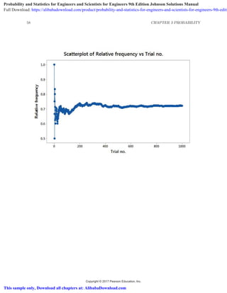
3.100 As the number of trials increases to a few hundred and beyond, the relative frequencies becomes much
less variable from trial to trail. It approaches the probability of the event 0.7.
Copyright © 2017 Pearson Education, Inc.](https://image.slidesharecdn.com/probability-and-statistics-for-engineers-and-scientists-for-engineers-9th-edition-johnson-solutions--200101130110/85/New-Perspectives-on-HTML5-CSS3-JavaScript-6th-Edition-Carey-Solutions-Manual-23-320.jpg)