1. Monte – machine learning in Python
Release 0.1.0
Roland Memisevic
May 9, 2008
Department of Computer Science
University of Toronto
Email: roland@cs.toronto.edu
Abstract
Monte (Python) is a machine learning framework written in Python. Its purpose is to facilitate the rapid development
of gradient-based learning machines, including neural networks, conditional random fields, logistic regression, and
others. This document describes the usage and a bit of the design philosophy behind Monte.
This document is currently in the making. If you miss parts of some sections now, there is a good chance that you
will find them if you check back tomorrow.
Contents
1 Installation 1
1.1 Getting Monte . . . . . . . . . . . . . . . . . . . . . . . . . . . . . . . . . . . . . . . . . . . . . . . 1
1.2 Installing Monte . . . . . . . . . . . . . . . . . . . . . . . . . . . . . . . . . . . . . . . . . . . . . . 2
2 Using the models 2
2.1 Models and trainers . . . . . . . . . . . . . . . . . . . . . . . . . . . . . . . . . . . . . . . . . . . . 2
2.2 Example: Constructing a simple conditional random field . . . . . . . . . . . . . . . . . . . . . . . . 3
Extension to nonlinear conditional random fields . . . . . . . . . . . . . . . . . . . . . . . . . . . . 4
3 Assembling models from components 5
3.1 Example: Constructing a linear regression model from scratch . . . . . . . . . . . . . . . . . . . . . 6
Checking the correctness of the model . . . . . . . . . . . . . . . . . . . . . . . . . . . . . . . . . . 8
Extension to non-linear regression . . . . . . . . . . . . . . . . . . . . . . . . . . . . . . . . . . . . 9
4 Summary of available models 9
5 Future 10
6 License 10
1 Installation
Monte is released under the license described in the file LICENSE, which is part of the Monte distribution.

2. This section describes where to get, and how to install Monte 0.1.0. If you look ahead, you will notice that this section
takes up far less than one page. This is not accidental. Monte 0.1.0 can usually be installed, and is ready-to-use within
a few minutes or less.
Which, again, is not by accident. Monte, deliberately, does not try to be an overblown new framework that dictates
how you solve your daily data-analysis tasks, or requires a 300-page manual describing its basic usage. (Monte would
have been written in a different language in that case anyway.) What Monte does try to provide is a collection of
re-usable components, classes and functions, that can make your life as a data-miner a bit easier.
1.1 Getting Monte
Monte is available at http://sourceforge.net/projects/montepython/. To get the most out of Monte, the packages Numpy
(Version 1.0 or later), Scipy and Matplotlib (Version 0.87 or later) should to be installed as well – if not present
already. Installing those packages is advisable anyway, if you are planning to ever do any serious data-analysis,
machine learning, or numerical processing with Python.
1.2 Installing Monte
Installing Monte is very simple: Just copy the main directory monte/ somewhere into your Python search path. Also
make sure that you have the numerical supporting packages listed in the previos section on your path. That’s all! You
should be ready to use Monte now.
2 Using the models
This section describes how to use and apply models that are defined in Monte.
2.1 Models and trainers
The two most important kinds of object in Monte are models and trainers. Models are learning machines, and trainers
are optimizers that can adapt a models’ parameters based on data. The interplay between models, trainers and data is
based on a few very simple conventions that we outline in the following.
Models are simply learning machines, that typically contain some parameters which need to be set based on training
data. Examples of Monte’s models are linear regression, neural networks and logistic regression. While Monte
provides these and some other readily defined models, Monte’s main goal is to make it easy to build your own models
from components. How to define new models using Monte components is described in detail in Section 3. This Section
focusses on using existing models, either pre-defined ones or self-made ones that were built previously using Monte
components.
A model in Monte can be defined as a simple Python class. A few conventions are used to define the interplay
between models and trainers, and these conventions determine what makes a Monte model class. By convention,
model parameters are contained in an attribute called params, and they are defined as a Numpy array of rank 1.
Trainers can access this array in order to adapt the parameters (more on this in a moment). Models furthermore contain
two methods that are needed by trainer-objects to optimize the parameters. The method grad returns the gradient of
the model’s objective with respect to its parameters; the method cost returns the model’s objective function (also
a function of the model’s parameters). While params and grad are always expected to be present in a model, the
method cost is not always present. The reason for this is that there can be models that do not have a well-defined
objective function, but that can be trained nevertheless using just their gradient-dynamics.
The presence of these attributes (member params, method cost, possibly method grad) is all that is required to
define a “model” in Monte’s terms. Any class that implements these attributes qualifies as a Monte model and can be
trained with a trainer object.
2 2 Using the models

3. A trainer in Monte is a simple Python class, too. Trainers are used to adapt a model’s parameters so as to minimize its
cost function. For this purpose, a model is registered with a trainer at the time that the trainer object is constructed.
Trainer objects are expected to take at least one argument in their init -method – the model that they are
supposed to optimize. Most trainers have a step-method, that performs a single step of gradient-based optimization.
The definition of “a step” can differ from trainer to trainer; it can mean one step of online gradient descent, or one
batch of conjugate gradients iterations, for example.
A trainer works by repeatedly calling its model’s cost and grad methods and modifying the model’s params
in order to minimize the model’s cost. There are no additional rule or conventions that define a proper trainer.
However, most trainers are derived from a super-class Trainer contained in monte.gym.trainer. That super-
class provides some convenience book-keeping that is often useful when defining a trainer.
In the following section we will take a look at an example. We use a readily defined model for this purpose. Most
readily defined models reside in monte.arch.
2.2 Example: Constructing a simple conditional random field
To get an idea of how Monte works, we will now take a look at the file ‘crf example.py’ in the subdirectory ‘examples’.
The example describes how to build a conditional random field (CRF) from scratch. CRF’s are simple probabilistic
models for predicting a whole collection of class-labels (a sequence in this case) simultaneously.1
Let us go through the example in a step-by-step fashion to see what is going on (everything is printed here, so you do
not actually have to go looking for the example in your Monte distribution right now):
from numpy import *
from pylab import *
from monte.arch.crf import ChainCrfLinear #all ready-to-use models
#reside in monte.arch
from monte.gym import trainer #everything to do with training resides in
#monte.gym
The file starts with a couple of import statements. Since we will be juggling arrays and numerical objects anyway, we
get the all the Numpy and Pylab definitions first (lines one and two).
More interesting are lines three and four: In line three we get the class ChainCrfLinear from the module
monte.arch.crf. The module ChainCrfLinear is one of several modules that live in the sub-package
monte.arch. Some siblings of the crf include, for example, the module knn, or the module autoencoder.
The class ChainCrfLinear is all we need from the module for now. It defines a linear chain conditional random
field. It contains the methods that are necessary to perform inference or otherwise apply the crf, and holds all the
parameters, and settings (such as the number of input-dimensions and number of classes), etc. (We will see how to
actually instantiate a ChainCrfLinear-object in a moment.)
In line four we import a trainer-module. It contains a set of trainer-classes, that can be used to train any
system, including our crf. Training a machine learning model usually amounts to performing some kind of numerical
optimization. Since there are many ways of performing such an optimization, there are also many different trainers.
Note also that, how you train a model is typically unrelated to how your model is defined. This is why trainers and
model-definitions are (usually) separated in Monte.
The trainer-module resides in the sub-package gym. The module contains a set of different trainers (some are good
for online-training, some are good for batch-training, some are good for models that don’t have an objective function,
some are good for other things). We will pick a trainer that’s good for our purpose in a moment. But first, let us look
at the next line:
mycrf = ChainCrfLinear(3,2)
1 We could have used any other kind of model, but CRF’s are kind of hot right now... Using another model, say a neural-network regression
model, the example would have looked almost the same. You are welcome to try this...
2.2 Example: Constructing a simple conditional random field 3

4. We instantiate our ChainCrfLinear-class, since a CRF is what we want to build. We pass in two parameters: The
number of input-dimensions, and the number of classes that each label can take on. These are the only two parameters,
that the ChainCrfLinear-class expects. To find out how to instantiate some other model, try help or take a look
at the model-definition.
Now that we have built a model, we can construct a trainer for the model. We do so by instantiating one of the
trainer-classes:
mytrainer = trainer.Conjugategradients(mycrf,5)
The trainer Conjugategradients uses scipy’s conjugate gradients-solver to do the job and is rela-
tively fast. If scipy was not available, we could have used a more self-contained trainer, such as
trainer.gradientdescentwithmomentum, that does not require any external packages.
The constructor for the trainer Conjugategradients expects two arguments: The first is the model that we want
our trainer to take care of. The second is the number of conjugate-gradient-steps each call of the trainer is supposed
to do. While the second argument is specific to this particular type of trainer, the first (the model) is common to all
trainers: We need to register the model that we want to train with the trainer object. Internally, what this means is that
the trainer object receives a pointer to the model’s parameter-vector. This parameter-vector is what is being updated
during training. The trainer repeatedly calls the model’s objective-function, and gradient (if available) to perform the
optimization.
Other trainer-objects might expect other additional arguments – again, the online-help, or a look at the class-definition,
should inform us accordingly.
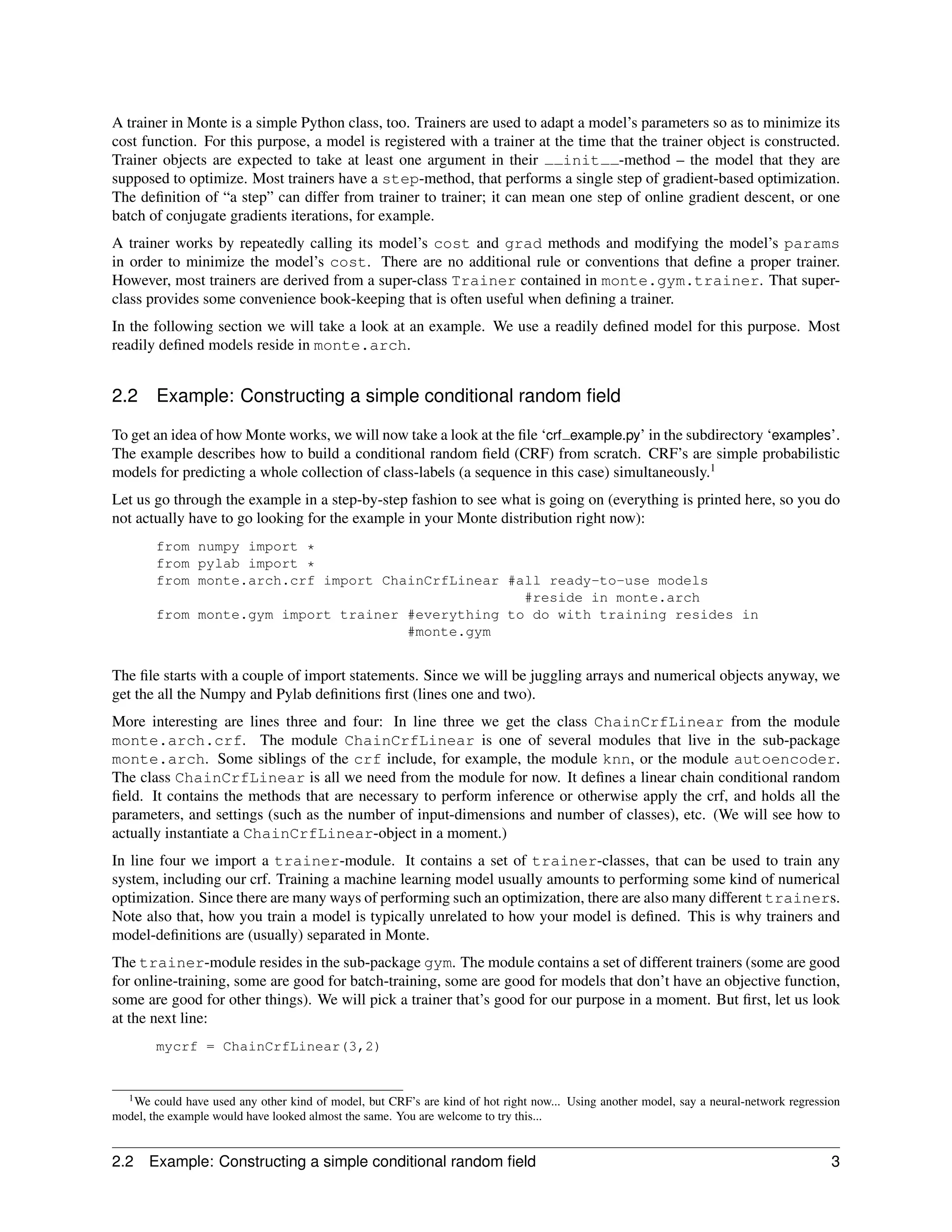
To see if the model works at all, let us produce some junk data now:
inputs = randn(10,3)
outputs = array([0,1,1,0,0,0,1,0,1,0])
We simply produce a sequence of ten three-dimensional random vectors. The ChainCrfLinear-class expects the
first dimension to be the ’time’-dimension (10 in our case), and the second dimension to be the input-space-dimension
(3 in our case). We also produce a sequence of (10) corresponding labels (also random, for the sake of demonstration).
The label-sequence is encoded using a rank-1-array. Each single class-label is encoded as an integer, with 0 being the
first class. This encoding is a convention that is used by other classification-type models in monte, too.
With some data at our hands we are now ready to train the model. For this end, all we need to do, is repeatedly call
the step()-method of the trainer. Since this is just a demonstration, we simply train for 20 steps now. (In a real
application, we would probably use a more reasonable stopping criterion – more on these later.)
for i in range(20):
mytrainer.step((inputs,outputs),0.001)
print mycrf.cost((inputs,outputs),0.001)
We pass two arguments to our trainer’s step()-method. All the trainer does is, (repeatedly) passing these on to the
cost- and gradient functions of the learning machine that we have registered with it previously. So it’s actually the
ChainCrfLinear-object that requires two arguments for training. The two arguments are a tuple containing inputs
and outputs (we also could have passed in a list of input-output-pairs, if we had several sequences to train on) and a
weightcost. Most parametric models in monte require a weightcost for training. The weightcost is a multiplier on the
weight-decay term that is used for regularization.
Calling the cost()-method (on the same data) Finally, we can apply the model on some random inputs. To get
the optimal class-labels on the test-inputs, we call the ChainCrfLinear’s viterbi()-method. (The viterbi-
algorithm is what’s needed to apply a crf. When dealing with a more standard-type of problem, such as regression or
simple classification, look for a method apply()):
4 2 Using the models

5. testinputs = randn(15,3)
predictions = mycrf.viterbi(testinputs)
print predictions
Extension to nonlinear conditional random fields
One benefit of Monte’s modular design is that many of its models can be easily modified or extended in various ways.
One way we can modify a crf, for example, is by defining its observation potentials to be a non-linear function instead
of using the common linear potential function. A model that does this is defined in the class ChainCrfNNIsl, which
resides in the same module as our chain crf above.
ChainCrfNNIsl uses a back-prop-network with one (sigmoid) hidden layer as the observation potential. (Other
extensions, such as those that redefine both the observation-potentials and the compatibility-potentials to be non-
linear, can be constructed quite easily, as well.) Why the strange name? ’NNIsl’ means ’neural network with the
structure: inputs–sigmoid–linear’. This kind of abbreviation is used at several places within Monte to denote various
types of neural network.
To train and apply this non-linear version of a crf, we can proceed just as we did before. We only need to replace the
statement that constructed our linear model previously by one that constructs a non-linear one now:
mynncrf = ChainCrfNNIsl(3,10,2)
The non-linear model expects a number of hidden units as its second argument, which we set to 10 here. We can define
a trainer just as before, since training is the same for non-linear and linear models:
mytrainer = trainer.Conjugategradients(mynncrf,5)
To train the model use calls to the trainer’s step-method, just as before:
mytrainer.step((inputs,outputs),0.001)
3 Assembling models from components
In this Section we take a look at how to assemble your own models using the components that Monte defines.
Monte uses a modular design-philosophy that relies to a large degree on error back-propagation. Error back-
propagation (often just “back-prop”) is a common algorithm for computing gradients to train learning machines.
It was initally invented for neural networks, but back-prop is useful in a much larger context and can be deployed
in a very wide variety of models. Back-prop learning is especially useful when implemented in an object-oriented
language. This observation is the basis for the great back-prop libraries available for the Lush-language2 developed by
Yann LeCun and Leon Bottou, the main inspiration behind Monte.
The basic idea behind back-prop learning is that it is easy to compute gradients in complicated systems composed
of multiple modules, as long as we can compute gradients of each module with respect to its inputs. This fact is
a simple consequence of the chain rule for differentiation, and it unfolds its full power when combined with object
oriented design: As long as we define modules such that they can compute derivatives with respect to their intputs
from derivatives with respect to their outputs, combining them to large, complex systems is simply a matter of sticking
2 http://lush.sourceforge.net/
5

6. the modules together. Just as the outputs of a composed system can be computed as a cascade of function evaluations,
gradients are computed simply as a cascade of gradient computations. That is, the chain-rule never needs to be evoked
explicitly.
To implement this idea, the back-prop modules in Monte contain four crucial elements, following a similar design in
Lush’s back-prop modules:
1. An fprop-method that computes its outputs from its inputs (short for “forward propagation”),
2. A bprop-method that computes the derivatives with respect to its inputs (from derivatives with respect to its
outputs; short for “backward propagation”),
3. A grad-method that computes the gradient with respect to its own parameters (from its inputs and the deriva-
tives with respect to its outputs)
4. A params-attribute that points to the module’s parameters (which are always a rank-1 Numpy-array).
The fprop-, bprop-, grad- and params-members can be found in practically every back-prop-module defined
in Monte. All back-prop modules are defined in the package monte.bp. Most back-prop modules also contain a
convenience-function called numparams, that computes the number of parameters that the module requires (and
thus the length of its parameter-array).
Given a back-prop system and some data, computing gradients for all modules contained in the system follows ba-
sically always the same procedure: We first compute a “forward-pass” by calling the modules’ fprop-methods. If
our system is composed of multiple modules, the outputs of one module will (obviously) be the inputs of one or more
other modules. The final module is often one that computes a cost, such as a squared reconstruction error.
After computing the forward-pass, we compute a “backward-pass” by computing all modules’ bprop-methods to
obtain derivatives with respect to their inputs. To do so, we need to reverse the order of calls that we used for
the forward-pass: This will make sure that a successor-module’s input-derivatives will be used by the predecessor-
module as output-derivatives – from which the predecessor computes its own inputs-derivatives, which become it’s
own predecessor’s outputs, etc.
Finally, after we completed the backward-pass, we can get each module’s parameter-gradients by calling their grad-
methods. The following code-snippet demonstrates this idea. It defines a complete, self-contained class (a model for
performing linear regression), that could be readily trained with a trainer-object and applied to some real data:
6 3 Assembling models from components

7. 3.1 Example: Constructing a linear regression model from scratch
from numpy import hstack
from pylab import randn
from monte import bp
class LinearRegression(object):
"""A simple linear regression class built with Monte back-prop
components.
"""
def __init__(self, numin, numout):
self.numin = numin
self.numout = numout
self.params = 0.01 * randn(bp.neuralnet.Linearlayer.numparams(numin, numout))
self.functionmodule = bp.neuralnet.Linearlayer(numin, numout, self.params)
self.costmodule = bp.cost.Squarederror()
def cost(self, inputs, outputs):
return self.costmodule.fprop(self.functionmodule.fprop(inputs), outputs)
def grad(self, inputs, outputs):
modeloutputs = self.functionmodule.fprop(inputs) #forward pass
self.costmodule.fprop(modeloutputs, outputs) #...
d_outputs = self.costmodule.bprop(modeloutputs, outputs) #backward pass
self.functionmodule.bprop(d_outputs, inputs) #...
return self.functionmodule.grad(d_outputs, inputs).sum(1) #compute gradient
def apply(self, inputs):
return self.functionmodule.fprop(inputs)
Let us go through the code step by step to see how it implements the strategy described above:
As mentioned in the previous section, any ready-to-train model should be a Python-class that contains at least a cost-
and a grad-method. Our model makes use of back-prop-learning to implement both of these as we describe in detail
in a moment. Note, that the model also defines an init and an apply-method for convenience of use.
The init -method contains some boilerplate. It initializes the model by (i) saving the number of input- and
output-dimensions (lines 1 and 2 in the method), (ii) making a parameter-array, filled with some small random values
using Pylab’s randn-function (line 3) and last but not least (iii) constructing the two back-prop modules, that our
model is supposed to use: One for computing a linear regression function and one for computing a reconstruction-cost
(lines 4 and 5). The linear regression function is taken from bp.neuralnet. which contains various components
useful in building neural networks. Here, we just use the class Linearlayer from that module, which computes a
simple (affine-)linear function. The cost module is taken from bp.cost.
One very important lesson to be learned from this example is the following: The model’s parameters (which, as
mentioned above, are saved in a Numpy-array) belong to the model. The model’s back-prop modules, in turn, get to
see only pointers to this parameter-array. And they receive these pointers at the time they are constructed (line 4 in the
example). Most back-prop modules expect a pointer to a parameter-array in their constructor3 . Later, we will show
how back-prop modules can be defined recursively by nesting back-prop modules inside other back-prop-modules. It
is important to keep in mind that in cases like these, owner-ship of the parameter-array always stays with the outer-most
3 The
fact that pointers, rather than copies, of the model’s parameters are being passed to back-prop-modules is crucial for learning, but happens
somewhat unconspicuously and implicitly, by making use of the fact that in Python function calls are by reference.
3.1 Example: Constructing a linear regression model from scratch 7

8. component. All sub-components receive only references to these parameters. In our case, the outer-most component
is our LinearRegression-class.
The other back-prop component that our class uses (bp.cost.Squarederror) does not take any parameters. It
does compute gradients with respect to its inputs nevertheless – these are always needed for computing gradients
further down.
The heart of our LinearRegression-class are the cost- and grad-methods. They are the methods that actually
implement the fprop-/bprop-scheme described above. The cost-method is straightforward. It simply computes a
short cascade of the fprop-methods on its back-prop components: Its function-module’s fprop computes a linear
function, its cost-modules fprop subsequently computes the resulting squared reconstruction error.
To compute gradients, we need to do a forward-pass followed by a back-ward pass, which is what the grad-method
does4 : It first computes the linear function to obtain the model’s guess as to what the correct outputs on the given inputs
are, followed by the cost-function. It saves the model-outputs in the variable modeloutputs (rather than returning it
like the cost-method). Saving the model-outputs is necessary, because we need them for the backward-pass.
The backward-pass follows right after we computed the forward-pass and calls the model’s back-prop components
in reversed order: First, we call the cost-modules’ bprop-method. This method expects the same arguments as the
corresponding fprop-call: The model-outputs and the desired (training) outputs. This is why we saved the model-
outputs before. The modules’ output is the derivative of the module with respect to its inputs (which in our case are the
model-outputs). We save these derivatives in a variable d outputs. Given the derivatives we can continue with the next
module in the backward-cascade: We call our function-modules bprop-method using d outputs and this modules’
inputs as arguments, and the back-ward pass is completed.
After completing the backward-pass we can call each module’s grad-method to obtain their gradients. Note, that
the only module containing any parameters in our case is the function module. We compute it’s gradient (last line in
grad) and sum it up over all input-cases, which we assume to be arranged columnwise in the input. Since this is the
only set of parameters that we use, we directly return the gradient. In case we had several modules with parameters,
we would first stack them into a single array. We will see an example of this below.
To complete our Linear Regression class we add an apply-method for convenience. This method simply applies
the learned function to new inputs by calling the function-components fprop-method. The result is a self-contained
linear regression class that we could register with a trainer and train and apply to real data. In practice we might want to
add a regularization term, for example a weight-decay, to the cost function and to its gradient. This is straightforward,
and we leave it as an exercise.
Note that in our example we never needed to explicitly compute any derivatives ourselves. While computing deriva-
tives would have been easy in this simple case, the possibility of assembling models from components without needing
to calculate any derivatives by hand will become extremely useful as soon we transition to more complex models.
Checking the correctness of the model
As a sanity check, to see whether the model does the right thing, let us compare the parameters it comes up with after
training to those that we obtain from using a more traditional approach to doing linear regression.
A more “traditional” way of performing linear regression is by minimizing squared reconstruction error using a closed
form solution. Say, we want to apply a model with 5-dimensional inputs and 1-dimensional outputs and we have
(columnwise) training data matrices X and Y for inputs and outputs, respectively. Here X is a 5 × N - and Y is a
1 × N -matrix, where N is the number of training cases. Generating some random data could be done like this:
4 Note that grad repeats the forward-pass that cost computes. If we can make sure that the trainer that we use to train the model always calls
cost before it calls grad, then we can also do without the forward-pass in grad. We shall discuss this topic in more detail later.
8 3 Assembling models from components

9. >>> X = randn(5, 1000) #create 1000 inputs
>>> w = randn(5) #create a linear model
>>> w
array([-0.56883823, -1.47482531, 1.21239073, -1.79361343, -0.64315871])
>>> Y = dot(w, X) + randn(1, 1000) #create the outputs
It is well-known that the optimal (in terms of squared error) linear function based on the training data has parameters
wlinreg = (XX T )−1 XY T . In Python, we can write this as
>>> dot(inverse(dot(X,X.T)),dot(X,Y.T)).T
array([[-0.55389647, -1.52445261, 1.17153374, -1.83514791, -0.68079122]])
We see that the solution is fairly similar to the actual parameters w. Now, to train our back-prop-module, we can
proceed as usual, by instantiating it, building a trainer and running it for a few steps:
>>> model = LinearRegression(5,1)
>>> trainer = monte.gym.trainer.Conjugategradients(model, 20)
>>> trainer.step((X,Y), 0.0)
Let us look at the model parameters to check what they look like after training:
>>> model.params
array([-0.55376029, -1.52260298, 1.16934185, -1.83290113, -0.68340035,
-0.0762695 ])
We see that the parameters are very similar to what the closed-form solution gives us. The model parameters have one
extra component, which is close to zero, and represents the affine part of the model. (To access the linear part w of our
model we could have als made use of the fact that it is exposed as a member w by the Linearlayer. The affine part
is exposed as the member b.)
Why doing linear regression in this involved back-prop-way in the first place, given that we can get the solution from
a one-liner? One reason is that with the linear back-prop model in place, we are just a stone’s throw away from much
more powerful (for example, non-linear or multi-layer) models, as we describe in the next section.
Extension to non-linear regression
The modularity makes it trivially easy to extend the model in order to obtain, for example, a non-linear version. Let
us consider a non-linear regression model using a simple multi-layer neural network, for example. What we need
to do is replace the linear function-module with a non-linear, neural network-based one. The back-prop compo-
nent SigmoidLinear has an interface that is almost exactly the same as the Linearlayer-component which
we used before. The only difference is that at construction-time the component expects one additional argument,
which is the number of units in its hidden layer. To use this component all we need to do is change a few lines in
init . The cost- and grad-methods stay exactly the same, because all the interfaces are the same. The new
init -method needs to take an additional argument (the number of hidden units) and replace the functionmodule
with SigmoidLinear:
3.1 Example: Constructing a linear regression model from scratch 9

10. class NonlinearRegression(object):
"""A simple non-linear regression class built with Monte back-prop
components.
"""
def __init__(self, numin, numhid, numout):
self.numin = numin
self.numhid = numhid
self.numout = numout
self.params = 0.01 * randn(bp.neuralnet.SigmoidLinear.numparams(numin, numhid, numout))
self.functionmodule = bp.neuralnet.SigmoidLinear(numin, numhid, numout, self.params)
self.costmodule = bp.cost.Squarederror()
#rest exactly the same as for LinearRegression
It is interesting to note that SigmoidLinear is itself composed of multiple sub-components, and it uses its com-
ponent’s forward- and backward propagation methods to do its work. (If interested, take a look at its definition in
‘monte/bp/neuralnet.py’.) However, since gradient-computations are always encapsulated within each component, so
we don not need to worry about them, when using the components.
In a similar fashion, we could use a three-layer network or any other type of component to define the function-module.
4 Summary of available models
This section provides a short summary of the currently available models in Monte.
Most of the learning methods are, similarly as the crf-example in the previous section, based on parametric models.
There are a few exceptions, for example, k-nearest neighbors or k-means, which contain their own specialized training
methods (if any). (See below for details on these and other models).
For the parametric models training has been deliberately separated from the definition of the models themselves. The
reason is that training often amounts to performing some form of numerical optimization, and there are many possible
ways of performing such an optimization. Which way is the best depends heavily on the application domain and
other factors that are completely independent of the model itself. Furthermore, optimization is an ’orthogonal’ line of
research, and there might be optimization approaches of which we don’t even know yet.
Monte’s directory layout is fairly simple. The main directory ‘monte/’ contains a couple of files and several subdirec-
tories. Each subdirectory has its own well-defined purpose.
Monte’s Directory layout
10 4 Summary of available models

11. Directory Purpose
bp/ This directory contains trainable ’back-prop’-components. Each of
these components contains an fprop-method, a bprop-method, and a
grad-method. Training of the components is done with error back-
propagation. The method fprop computes the response of the component
wrt. its input. The method bprop computes the derivative of some error-
function with respect to the component’s inputs from the derivative wrt.
to it’s outputs. The method grad computes the derivative of the error wrt.
the component’s parameters.
models/ This directory holds trainable modules, that is components that contain
cost function and gradient and can be trained using trainer objects.
models/contrastive/ Many common learning machines are ’contrastive’: They are trained us-
ing positive and negative examples. This directory contains the definiton
for an abstract class ’contrastive’ and a set of sub-classes that are trained
using the contrastive learning paradigm. The sub-directory ’scorefunc’
contains a wide variety of score-functions from which complex learn-
ing machines can be constructed. Many of these score-functions make
use of the back-prop-components defined in the directory bp. While
the idea of contrastive learning encompasses a surprisingly large num-
ber of learning machines, the goal is to include alternative learning ap-
proachen over time, each populating its own directory within models,
besides ‘contrastive/’.
arch/ All top level architectures are placed here – ie. fully functional systems
that can be trained with a trainer object and that can be applied without
much effort to real data.
gym/ The definition of models, and of mechanisms for training these, has been
deliberately separated in Monte. The directory gym contains trainer-
classes, that are registered with a model at construction time, and are
used to train the model.
examples/ This directory contains simple example-scripts, that illustrate various as-
pects of Monte.
util/ Helper functions- and classes are placed here. These include, for exam-
ple fuctions for normalizing data, computing a numerically stable ’log-
sumexp’, etc.
5 Future
6 License
LICENSE AGREEMENT FOR MONTE 0.1.0
Monte is distributed under the Python Software Foundation (PSF) license, which permits commercial and noncom-
mercial free use and redistribution as long as the conditions below are met.
1. This LICENSE AGREEMENT is between Roland Memisevic (”RM”), and the Individual or Organization (”Li-
censee”) accessing and otherwise using Monte software in source or binary form and its associated documentation.
2. Subject to the terms and conditions of this License Agreement, RM hereby grants Licensee a nonexclusive, royalty-
free, world-wide license to reproduce, analyze, test, perform and/or display publicly, prepare derivative works, dis-
tribute, and otherwise use Monte 0.1.0 alone or in any derivative version, provided, however, that RM’s License
Agreement and RM’s notice of copyright, i.e., ”Copyright (c) 2007 Roland Memisevic; All Rights Reserved” are
retained in Monte 0.1.0 alone or in any derivative version prepared by Licensee.
3. In the event Licensee prepares a derivative work that is based on or incorporates Monte 0.1.0 or any part thereof,
11

12. and wants to make the derivative work available to others as provided herein, then Licensee hereby agrees to include
in any such work a brief summary of the changes made to Monte 0.1.0.
4. RM is making Monte 0.1.0 available to Licensee on an ”AS IS” basis. RM MAKES NO REPRESENTATIONS OR
WARRANTIES, EXPRESS OR IMPLIED. BY WAY OF EXAMPLE, BUT NOT LIMITATION, RM MAKES NO
AND DISCLAIMS ANY REPRESENTATION OR WARRANTY OF MERCHANTABILITY OR FITNESS FOR
ANY PARTICULAR PURPOSE OR THAT THE USE OF MONTE 0.1.0 WILL NOT INFRINGE ANY THIRD
PARTY RIGHTS.
5. RM SHALL NOT BE LIABLE TO LICENSEE OR ANY OTHER USERS OF MONTE 0.1.0 FOR ANY IN-
CIDENTAL, SPECIAL, OR CONSEQUENTIAL DAMAGES OR LOSS AS A RESULT OF MODIFYING, DIS-
TRIBUTING, OR OTHERWISE USING MONTE 0.1.0 OR ANY DERIVATIVE THEREOF, EVEN IF ADVISED
OF THE POSSIBILITY THEREOF.
6. This License Agreement will automatically terminate upon a material breach of its terms and conditions.
7. Nothing in this License Agreement shall be deemed to create any relationship of agency, partnership, or joint
venture between RM and Licensee. This License Agreement does not grant permission to use RM trademarks or trade
name in a trademark sense to endorse or promote products or services of Licensee, or any third party.
8. By copying, installing or otherwise using Monte 0.1.0 Licensee agrees to be bound by the terms and conditions of
this License Agreement.
12 6 License