This document discusses monopoly and natural monopoly. It defines a monopoly as a single supplier of a product in a market. Unlike perfect competition, a monopolist faces a downward sloping demand curve. The marginal revenue curve for a monopolist is downward sloping and has the same y-intercept and twice the slope of the demand curve. A monopolist produces where marginal revenue equals marginal cost and charges the price on the demand curve. This leads to monopoly profits, consumer surplus, and deadweight loss. A natural monopoly exists when economies of scale lead to declining average total costs over the relevant output range, making it most efficient for a single firm to produce the entire output. Natural monopolies are often regulated by governments setting price limits like average

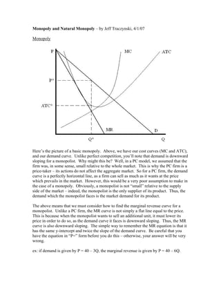
1. Monopoly and Natural Monopoly – by Jeff Traczynski, 4/1/07
Monopoly
Here’s the picture of a basic monopoly. Above, we have our cost curves (MC and ATC),
and our demand curve. Unlike perfect competition, you’ll note that demand is downward
sloping for a monopolist. Why might this be? Well, in a PC model, we assumed that the
firm was, in some sense, small relative to the whole market. This is why the PC firm is a
price-taker – its actions do not affect the aggregate market. So for a PC firm, the demand
curve is a perfectly horizontal line, as a firm can sell as much as it wants at the price
which prevails in the market. However, this would be a very poor assumption to make in
the case of a monopoly. Obviously, a monopolist is not “small” relative to the supply
side of the market – indeed, the monopolist is the only supplier of its product. Thus, the
demand which the monopolist faces is the market demand for its product.
The above means that we must consider how to find the marginal revenue curve for a
monopolist. Unlike a PC firm, the MR curve is not simply a flat line equal to the price.
This is because when the monopolist wants to sell an additional unit, it must lower its
price in order to do so, as the demand curve it faces is downward sloping. Thus, the MR
curve is also downward sloping. The simple way to remember the MR equation is that it
has the same y-intercept and twice the slope of the demand curve. Be careful that you
have the equation in “P=” form before you do this – otherwise, your answer will be very
wrong.
ex: if demand is given by P = 40 – 3Q, the marginal revenue is given by P = 40 – 6Q.

2. Mathematical digression: why is this relationship between demand and marginal revenue
true? Well, marginal revenue is the change in total revenue divided by the change in
quantity. Let demand be given by D: P = aQ + b. Thus we have:
Total Revenue (TR) = PQ = (aQ + b)Q = aQ2 + bQ
Now we want to take the derivative of TR with respect to Q, so we have:
dTR/dQ = 2aQ + b = MR.
Comparing this against our original demand equation, we see that the marginal revenue
equation does indeed have the same y-intercept and twice the slope. If this digression
helps you see why this relationship is true, great. If not, don’t worry about it, but do
remember that it’s “same y-intercept, twice the slope”.
Monopolists (like every other firm) set MR = MC, marginal revenue equal to marginal
cost, to determine the optimal quantity to produce (Q*). In order to find the price the
monopolist will charge, we then go up to the demand curve to see how much consumers
are willing to pay for quantity Q*. The monopolist may charge this price because it is the
only supplier in the market, so there are no other firms to help bring the price down to the
minimum of ATC as is the case in perfect competition.
Now that we have P* and Q*, we can easily find ATC* as in the above picture. Thus, we
can now find monopoly profits, consumer surplus, and deadweight loss.

3. Here, we have colored in our previous picture to highlight the appropriate areas.
Monopoly profits are in green. Profits are calculated in the same way as we did before in
perfect competition. We find the difference between the total revenue and total cost
boxes, or we consider the difference between the price which the monopolist receives for
its product and its average total costs, multiplied by the quantity it sells. Thus, we have:
Profits = (P* - ATC*) x Q*
Consumer surplus is the blue area above. CS is defined as before – it’s the area below
the demand curve and above the price which consumers pay for the product. Here, the
price which consumers pay is clearly P*, so we have:
CS = ([(y-intercept of D) – P*] x Q*)/2
Deadweight loss is in grey above. Here, there is no straightforward equation for DWL,
because the bottom of the area is actually curved. This means that in order to calculate it
directly, we would have to integrate the area (and those of you who have done this before
know that integrating over an area between lines is even trickier than traditional
integration relative to the x-axis). So while you will not be expected to find this area
numerically in the general case, you should still be able to find it on the diagram.
Let’s work through a numerical example so you can see how this works. This example is
the sort of problem which shows up on tests a lot due to its mathematical simplicity.
ex: (Constant marginal costs, zero fixed costs)
Let demand be given by D: P = 100 – Q, MC = 20. Also, assume that the firm has no
fixed costs (FC = 0). Find the monopoly profits, CS, and DWL.
First, we find the equation for MR. As we have the equation for demand, we know that
MR has the same y-intercept but twice the slope. So MR: P = 100 – 2Q.
We know that MC = 20, but we also know that in order to calculate profits, we’re going
to need the ATC curve. So how do we find it? Well, let’s try to build it from the
information we have. Consider the first unit. We know that there are no fixed costs, and
MC = 20, so the total cost of making the first unit is 20, so the ATC is 20. Now consider
the second unit. Again, no fixed costs, and the cost of making the second unit is 20. So
the total cost for making two units is 40, so the ATC is again 20. Thus, we see that in the
case of constant marginal costs and zero fixed costs, the ATC curve is the same as the
MC curve. This is the critical insight of this example, as it allows us to calculate the
desired quantities with simple areas. So armed with this knowledge, we can now draw
the picture below to represent this situation. And from here, it is straightforward to
compute profits, CS, and DWL. Thus we have:
Profits = (60 – 20) x 40 = $1600
CS = [(100 – 60) x 40]/2 = $800
DWL = [(60 – 20) x (80 – 40)]/2 = $800

4. Natural Monopoly
So now that we’ve dealt with the idea of monopoly, what are the important features of
natural monopoly? Here’s the official definition.

5. Natural Monopoly: a monopoly created and sustained by economies of scale over the
relevant range of output for the industry.
The phrase “over the relevant range of output” is the operative one here. In a subtle and
important sense, natural monopoly is really a statement about demand and industry costs,
not market structures. For an example, consider the above picture, and assume that the
product is supplied by a monopolist. If demand for this product is given by D1, then the
industry is a natural monopoly. If demand is D2, then we have a regular monopoly.
An equivalent way to think about natural monopolies is through the cost structure.
Remember that MC must run through the minimum of ATC – so if ATC is falling, then
MC is below ATC. This means that if we think about the total costs of the industry for
producing a given quantity Q*, then the costs are lowest with only one firm producing the
output.
The above picture illustrates this idea. If one firm produces quantity Q*, then the total
costs for this industry are the red areas. If two firms each produce Q*/2, then we have the
same total quantity of output, but the total costs of the industry are the red areas plus the
orange areas. This is because the costs for the first firm are the left hand red and orange
areas, and as the second firm is identical to the first, the costs for the industry are twice
the costs of the first firm. The important thing to take away from this is that the total
industry costs rise as the number of firms increases if ATC is falling over the relevant
range of output. Thus, it is most efficient for society if there’s only one producer in this
industry – so having a monopoly in this industry is therefore “natural”. A common
example of natural monopoly is public utilities (electricity, water, cable) due to the high
cost of building a network of pipes or wires.

6. What do we do with natural monopolies? We could find P* and Q* and profits, and
that’s all done in exactly the same way as we did it above for a regular monopoly. The
main topic related to natural monopolies is that of regulation. Under regulation schemes,
the government forces the natural monopolist to provide its product to consumers at a
price fixed by the government. There are two prices which we wish to consider here –
price = ATC (average cost pricing) and price = MC (marginal cost pricing). Here, the
subscripts denote the type of regulation imposed on the market.
Each type of regulation has its pluses and minuses. Under average cost pricing, ATC =
P, so the profits of the natural monopolist are zero. However, we can see from the picture
that we still have deadweight loss, as we are not producing the socially optimal quantity
of output. This DWL, as before, must be the area between the demand curve, Qatc, and
MC. Remember, the socially optimal quantity of output is equal to the quantity which is
produced by a perfectly competitive industry, where P = MC. Therefore, under marginal
cost pricing, we are producing the optimal quantity of output. However, notice that the
firm is then making negative profits equal to (ATCmc – Pmc) x Qmc, so they do not want to
stay in business.
So what do we do? Well, if we set P = ATC, then our firm will stay in business, but we
lose out by having DWL. If we set P = MC, then we have no DWL, but we can only
keep our monopoly in business by giving them a subsidy equal to their negative profits
(as this would make their profits zero). And in order to have the money to subsidize the
monopoly, we have to put taxes on other markets to raise revenue. So which one we
ultimately pick should depend on the DWL we may impose on other markets. 1 In most
1
I say “may” here because of the possibility of using Pigouvian taxes on markets with externalities. Don’t
worry about this for now – we’ll cover this topic in the last part of the course.

7. cases, governments tend to go with average cost pricing because getting the public to
approve subsidies for monopolists is often politically difficult. So while marginal cost
pricing is the efficient solution in that it produces no DWL in this market, average cost
pricing is the most common practical solution applied to real natural monopolies. If you
read your utility bills closely, you’ll notice that there are occasionally notices about
“public hearings” concerning rates – these are opportunities for the utility company to
present evidence and demonstrate their costs to government officials, while the public
can comment on the effects any rate changes would have on their lives. Thus, while
natural monopolies are not common in the real world, the proper regulation of such firms
is an important function of the government.