Module 6: SupervisedLearning – Classification:
Logistic Regression, Decision Trees, Support Vector Machines, Performance
Metrics: Precision, Recall, F1-Score, ROC-AUC, Handling Class Imbalance:
SMOTE, Weighted Loss Functions.
2.
Supervised Learning:
• SupervisedLearning is a type of Machine Learning where the model is
trained on a labeled dataset — meaning each training example is
paired with an output label. The goal is for the model to learn the
mapping from inputs to the correct output.
• Within supervised learning, there are two main types:
• Classification (categorical output)
• Regression (continuous output)
3.
What is Classification?
InClassification, the aim is to predict a categorical label — that is, to
assign input data into one of a finite number of discrete classes or
categories.
• Input: Features (X)
• Output: Category Label (Y)
Examples:
• Email spam detection (Spam or Not Spam)
• Image recognition (Cat, Dog, or Bird)
• Medical diagnosis (Disease A, Disease B, or Healthy)
4.
Common Classification Algorithms:
AlgorithmBrief Description
Logistic Regression Predicts probability of a class.
Decision Trees Tree-like model of decisions.
Random Forest Ensemble of decision trees.
k-Nearest Neighbor (k-NN) Classifies based on majority among neighbors.
Support Vector Machines (SVM) Finds hyperplane that best separates classes.
Naïve Bayes Based on Bayes’ theorem and feature independence.
Neural Networks Complex models mimicking the human brain.
5.
Key Points
•Training Data:Data used to train the model.
•Testing Data: Data used to evaluate the model.
•Overfitting: Model performs well on training data but poorly on new data.
•Underfitting: Model performs poorly on both training and new data.
•Confusion Matrix: Table used to evaluate performance.
•Accuracy, Precision, Recall, F1-Score: Common evaluation metrics.
•Classification Types:
• Binary Classification: Only two classes (e.g., Yes/No, True/False).
• Multi-class Classification: More than two classes (e.g., Apple, Banana, Orange).
• Multi-label Classification: Each input can belong to multiple classes at the same time
(e.g., a document that is both “Sports” and “Politics”).
6.
Examples
1. Email SpamDetection
• Input Features: Email content, sender address, presence of
specific keywords.
• Output Classes: "Spam" or "Not Spam" (Binary
Classification)
2. Medical Diagnosis
• Input Features: Patient symptoms, age, test results.
• Output Classes: Disease types such as "Diabetes",
"Hypertension", "Healthy" (Multi-class Classification)
3. Image Recognition
• Input Features: Pixel values of an image.
• Output Classes: "Cat", "Dog", "Bird", etc. (Multi-class
Classification)
. Loan Approval System
• Input Features: Applicant income, credit score,
employment status.
• Output Classes: "Approved" or "Rejected" (Binary
Classification)
5. Sentiment Analysis
• Input Features: Text of a review or tweet.
• Output Classes: "Positive", "Negative", "Neutral" (Multi-
class Classification)
6. Self-driving Car – Traffic Sign Recognition
• Input Features: Camera images of road signs.
• Output Classes: "Stop", "Yield", "Speed Limit 60", etc.
(Multi-class Classification)
7. Music Genre Classification
• Input Features: Audio features like tempo, rhythm, pitch.
• Output Classes: "Pop", "Rock", "Jazz", "Classical" (Multi-
class Classification)
7.
Logistic regression
• Logisticregression is a supervised machine learning algorithm used for
classification tasks where the goal is to predict the probability that an
instance belongs to a given class or not.
• It is commonly used for binary categorization-related problems.
• In logistic regression, linear regression output is transformed into a
probability value using the sigmoid function.
• Logistic regression predicts the output of a categorical dependent variable.
Therefore, the outcome must be a categorical or discrete value.
• It can be either Yes or No, 0 or 1, true or False, etc. but instead of giving the
exact value as 0 and 1, it gives the probabilistic values which lie between 0
and 1.
• In Logistic regression, instead of fitting a regression line, we fit an “S” shaped
logistic function, which predicts two maximum values (0 or 1).
8.
Types of LogisticRegression
• Logistic Regression can be classified into three types:
• Binomial: In binomial Logistic regression, there can be only two
possible types of the dependent variables, such as 0 or 1, Pass or Fail,
etc.
• Multinomial: In multinomial Logistic regression, there can be 3 or
more possible unordered types of the dependent variable, such as
“cat”, “dogs”, or “sheep”
• Ordinal: In ordinal Logistic regression, there can be 3 or more
possible ordered types of dependent variables, such as “low”,
“Medium”, or “High”.
9.
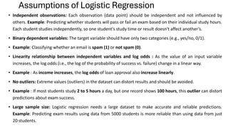
Assumptions of LogisticRegression
• Independent observations: Each observation (data point) should be independent and not influenced by
others. Example: Predicting whether students will pass or fail an exam based on their individual study hours.
Each student studies independently, so one student's study time or result doesn't affect another’s.
• Binary dependent variables: The target variable should have only two categories (e.g., yes/no, 0/1).
• Example: Classifying whether an email is spam (1) or not spam (0).
• Linearity relationship between independent variables and log odds : As the value of an input variable
increases, the log odds (i.e., the log of the probability of success vs. failure) change in a linear way.
• Example : As income increases, the log odds of loan approval also increase linearly.
• No outliers: Extreme values (outliers) in the dataset can distort results and should be avoided.
• Example : If most students study 2 to 5 hours a day, but one record shows 100 hours, this outlier can distort
predictions about exam success.
• Large sample size: Logistic regression needs a large dataset to make accurate and reliable predictions.
Example: Predicting exam results using data from 5000 students is more reliable than using data from just
20 students.
10.
Understanding Sigmoid Function
•The sigmoid function is a mathematical function used to map the predicted
values to probabilities.
• It maps any real value into another value within a range of 0 and 1.
• The value of the logistic regression must be between 0 and 1, which cannot go
beyond this limit, so it forms a curve like the “S” form.
• The S-form curve is called the Sigmoid function or the logistic function.
• In logistic regression, we use the concept of the threshold value, which defines
the probability of either 0 or 1.
• Such as values above the threshold value tends to 1, and a value below the
threshold values tends to 0.
11.
Sigmoid Function Example
•The sigmoid function maps any real number to a value between 0 and
1, making it ideal for converting raw outputs of a model into
probabilities.
12.
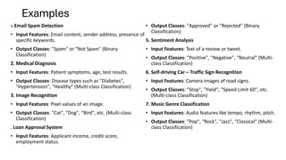
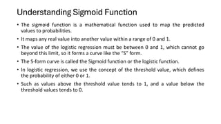
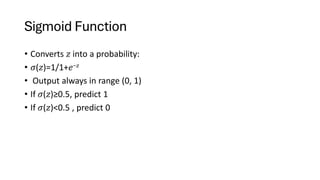
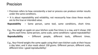
Example: Predicting ifa student passes or fails
Let’s say we have a model to predict if a student will pass (1) or fail (0) based on their study hours.
Suppose the linear output is:
• z=1.2
• Apply the sigmoid function:
• σ(1.2)=1/(1+e−1.2) ≈0.768
•This means there's a 76.8% chance the student will pass.
•If our threshold is 0.5, then 0.768 > 0.5 → prediction = pass (1).
•The blue S-curve shows how input values (z) are mapped to probabilities between 0 and 1.
•The red dashed line at 0.5 represents the typical threshold used to decide between class 0 or 1.
•Values of z > 0 give probabilities above 0.5 (classified as 1), and z < 0 gives probabilities below 0.5
(classified as 0).
13.
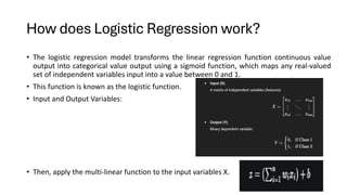
• The logisticregression model transforms the linear regression function continuous value
output into categorical value output using a sigmoid function, which maps any real-valued
set of independent variables input into a value between 0 and 1.
• This function is known as the logistic function.
• Input and Output Variables:
• Then, apply the multi-linear function to the input variables X.
How does Logistic Regression work?
14.
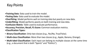
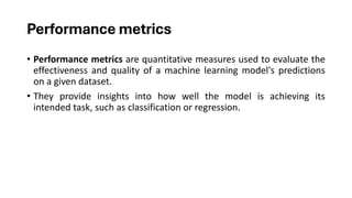
• Here xiis the I th observation of X, wi=[w1,w2,w3,⋯,wm] is the
weights or Coefficient, and b is the bias term also known as intercept.
simply this can be represented as the dot product of weight a
• z=w⋅X+b bias. Which is a linear regression.
Linear Function
• Combine inputs linearly:
• z=w⋅X+b
• Where:
• w = weights
• X = input features
• b = bias (intercept)
15.
Sigmoid Function
• Converts𝑧 into a probability:
• 𝜎(𝑧)=1/1+𝑒−𝑧
• Output always in range (0, 1)
• If 𝜎(𝑧)≥0.5, predict 1
• If 𝜎(𝑧)<0.5 , predict 0
16.
Log-Odds and Odds
•Odds represent the ratio of the probability
of an event happening to the event not
happening:
Odds=p(x)/1−p(x)
Example: If p(x)=0.8, then
• Odds=0.8/0.2=4
• The event is 4 times more likely to happen
than not.
Why Use Log-Odds
The logarithm of odds (log-odds) linearizes the
relationship :
log(𝑝(𝑥)/1−𝑝(𝑥))=𝑤⋅𝑋+𝑏
Odds:
p(x)/1−p(x)=ez
•Log-Odds:
log(p(x)/1−p(x))=z=w⋅X+b
• Logistic Regression models log-odds linearly.
• Final Equation of Logistic Regression
• p(X;w,b)=1/1+e−(w⋅X+b)
• This gives the predicted probability that
Y=1
This transformation allows us to:
• Model classification problems using linear
functions
• Avoid probability boundaries (0 and 1) when
learning
• Use linear regression techniques safely in a
classification context
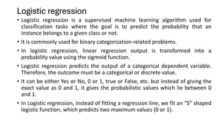
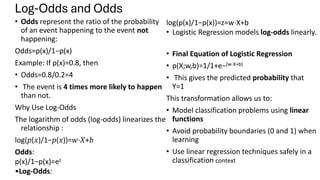
Summary
•Logistic Regression →for binary classification
•Uses sigmoid function to map output to [0, 1]
•Interprets result as probability
•Linear model applied to log-odds
19.
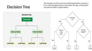
Decision Trees
• ADecision Tree is a supervised machine learning algorithm used for
both classification and regression tasks. It represents decisions and
their possible consequences in a tree-like structure,
• where:
• Root Node is the starting point that represents the entire dataset.
• Branches: These are the lines that connect nodes. It shows the flow
from one decision to another.
• Internal Nodes are Points where decisions are made based on the
input features.
• Leaf Nodes: These are the terminal nodes at the end of branches that
represent final outcomes or predictions
20.
Decision Tree
The exampleof a binary tree for predicting whether a person is
fit or unfit providing various information like age, eating habits
and exercise habits, is given below −
21.
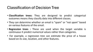
Classification of DecisionTree
• Classification trees: They are designed to predict categorical
outcomes means they classify data into different classes.
• They can determine whether an email is “spam” or “not spam” based
on various features of the email.
• Regression trees : These are used when the target variable is
continuous It predict numerical values rather than categories.
• For example, a regression tree can estimate the price of a house
based on its size, location, and other features.
22.
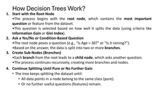
How Decision TreesWork?
1. Start with the Root Node
•The process begins with the root node, which contains the most important
question or feature from the dataset.
•This question is selected based on how well it splits the data (using criteria like
Information Gain or Gini Index).
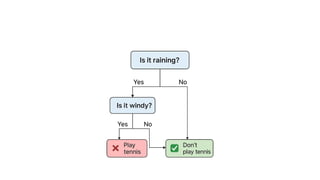
2. Ask a Yes/No or Condition-Based Question
•The root node poses a question (e.g., “Is Age > 30?” or “Is it raining?”).
•Based on the answer, the data is split into two or more branches.
3. Create Sub-Nodes (Branches)
•Each branch from the root leads to a child node, which asks another question.
•The process continues recursively, creating more branches and nodes.
4. Continue Splitting Until Pure or No Further Gain
• The tree keeps splitting the dataset until:
• All data points in a node belong to the same class (pure).
• Or no further useful questions (features) remain.
23.
Cont…
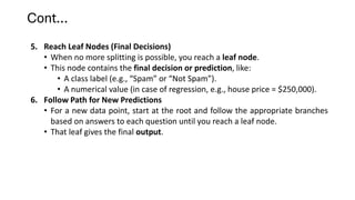
5. Reach LeafNodes (Final Decisions)
• When no more splitting is possible, you reach a leaf node.
• This node contains the final decision or prediction, like:
• A class label (e.g., “Spam” or “Not Spam”).
• A numerical value (in case of regression, e.g., house price = $250,000).
6. Follow Path for New Predictions
• For a new data point, start at the root and follow the appropriate branches
based on answers to each question until you reach a leaf node.
• That leaf gives the final output.
24.
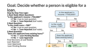
Goal: Decide whethera person is eligible for a
loan.
Step-by-Step Tree Logic:
1.Root Node (Main Question):
"Is the applicant's income > ₹50,000?"
•If Yes → go to next question.
•If No → Loan Rejected (leaf node).
2.Next Question:
"Is the credit score > 700?"
•If Yes → go to next question.
•If No → Loan Rejected (leaf node).
3.Next Question:
"Does the applicant have existing loans?"
•If Yes → Loan Pending Review
•If No → Loan Approved
Final Decisions at Leaf Nodes:
Loan Rejected
Loan Approved
Loan Pending Review
25.
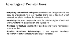
Advantages of DecisionTrees
• Simplicity and Interpretability: Decision trees are straightforward and
easy to understand. You can visualize them like a flowchart which
makes it simple to see how decisions are made.
• Versatility: It means they can be used for different types of tasks can
work well for both classification and regression
• No Need for Feature Scaling: They don’t require you to normalize or
scale your data.
• Handles Non-linear Relationships: It can capture non-linear
relationships between features and target variables.
26.
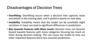
Disadvantages of DecisionTrees
• Overfitting: Overfitting occurs when a decision tree captures noise
and details in the training data, and it perform poorly on new data.
• Instability: Instability means that the model can be unreliable slight
variations in input can lead to significant differences in predictions.
• Bias towards Features with More Levels: Decision trees can become
biased towards features with many categories focusing too much on
them during decision-making. This can cause the model to miss out
other important features led to less accurate predictions .
27.
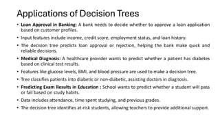
Applications of DecisionTrees
• Loan Approval in Banking: A bank needs to decide whether to approve a loan application
based on customer profiles.
• Input features include income, credit score, employment status, and loan history.
• The decision tree predicts loan approval or rejection, helping the bank make quick and
reliable decisions.
• Medical Diagnosis: A healthcare provider wants to predict whether a patient has diabetes
based on clinical test results.
• Features like glucose levels, BMI, and blood pressure are used to make a decision tree.
• Tree classifies patients into diabetic or non-diabetic, assisting doctors in diagnosis.
• Predicting Exam Results in Education : School wants to predict whether a student will pass
or fail based on study habits.
• Data includes attendance, time spent studying, and previous grades.
• The decision tree identifies at-risk students, allowing teachers to provide additional support.
29.
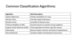
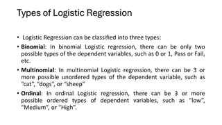
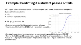
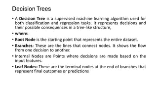
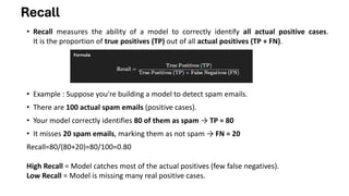
import pandas aspd
from sklearn.model_selection import train_test_split
from sklearn.tree import DecisionTreeClassifier
from sklearn.metrics import accuracy_score,
classification_report, confusion_matrix
from sklearn import preprocessing
import matplotlib.pyplot as plt
from sklearn import tree
# Sample Loan Approval Data (replace with your actual
data)
data = {
'Credit_Score': ['Poor', 'Fair', 'Good', 'Excellent',
'Good', 'Fair', 'Excellent', 'Poor', 'Good', 'Excellent'],
'Income': [25000, 40000, 60000, 80000, 55000,
35000, 90000, 30000, 70000, 100000],
'Debt_to_Income': [0.5, 0.4, 0.2, 0.1, 0.3, 0.6, 0.15,
0.55, 0.25, 0.05],
'Loan_Amount': [5000, 15000, 25000, 40000, 20000,
10000, 50000, 8000, 30000, 60000],
'Loan_Term': ['Short', 'Medium', 'Long', 'Short',
'Medium', 'Short', 'Long', 'Short', 'Medium', 'Long'],
'Property_Value': [80000, 150000, 300000, 500000,
250000, 120000, 600000, 100000, 350000, 750000],
'Loan_Approved': ['No', 'No', 'Yes', 'Yes', 'Yes', 'No',
'Yes', 'No', 'Yes', 'Yes']
}
df = pd.DataFrame(data)
# Convert categorical features to numerical using Label
Encoding
label_encoder = preprocessing.LabelEncoder()
df['Credit_Score'] =
label_encoder.fit_transform(df['Credit_Score'])
df['Loan_Term'] =
label_encoder.fit_transform(df['Loan_Term'])
df['Loan_Approved'] =
label_encoder.fit_transform(df['Loan_Approved']) #
Yes: 1, No: 0
# Separate features (X) and target (y)
X = df.drop('Loan_Approved', axis=1)
y = df['Loan_Approved']
# Split data into training and testing sets
X_train, X_test, y_train, y_test = train_test_split(X, y,
test_size=0.3, random_state=42)
# Initialize and train the Decision Tree Classifier
dt_classifier =
DecisionTreeClassifier(random_state=42)
dt_classifier.fit(X_train, y_train)
# Make predictions on the test set
y_pred = dt_classifier.predict(X_test)
# Evaluate the model
accuracy = accuracy_score(y_test, y_pred)
print(f"Accuracy: {accuracy:.2f}")
print("nClassification Report:")
print(classification_report(y_test, y_pred))
print("nConfusion Matrix:")
print(confusion_matrix(y_test, y_pred))
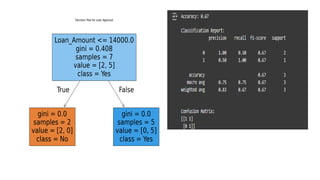
# Visualize the Decision Tree (requires graphviz to be
installed)
plt.figure(figsize=(15, 10))
tree.plot_tree(dt_classifier,
feature_names=X.columns, class_names=['No', 'Yes'],
filled=True)
plt.title("Decision Tree for Loan Approval")
plt.show()
31.
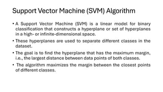
Support Vector Machine(SVM) Algorithm
• A Support Vector Machine (SVM) is a linear model for binary
classification that constructs a hyperplane or set of hyperplanes
in a high- or infinite-dimensional space.
• These hyperplanes are used to separate different classes in the
dataset.
• The goal is to find the hyperplane that has the maximum margin,
i.e., the largest distance between data points of both classes.
• The algorithm maximizes the margin between the closest points
of different classes.
32.
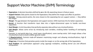
Support Vector Machine(SVM) Terminology
• Hyperplane: A decision boundary defined by w·x + b = 0, separating classes in feature space.
• Support Vectors: Data points closest to the hyperplane; they define the margin and affect its position.
• Example : Among several points, the ones closest to the separating line are support vectors — they define
the margin.
• Margin: The gap between the hyperplane and support vectors; SVM maximizes this for better separation.
• Kernel: A function that transforms input data into a higher-dimensional space to handle non-linear
separation.
• Hard Margin: A strict boundary that perfectly separates data without any misclassifications.
• Soft Margin: Allows some errors by introducing slack variables, enabling better handling of overlapping
classes.
• Example: In real-world data (e.g., email spam classification), some overlap exists. Soft margin allows a few
misclassified emails to build a better general model.
• C (Regularization): Controls trade-off between maximizing margin and allowing misclassifications; high C
means fewer errors.
• Hinge Loss: A function that penalizes points inside the margin or on the wrong side of the hyperplane.
• Dual Problem: An optimization approach using Lagrange multipliers, enabling kernel use and efficient
computation.
33.
How does SupportVector Machine Algorithm
Work?
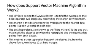
• The key idea behind the SVM algorithm is to find the hyperplane that
best separates two classes by maximizing the margin between them.
• This margin is the distance from the hyperplane to the nearest data
points (support vectors) on each side.
• The best hyperplane, also known as the “hard margin,” is the one that
maximizes the distance between the hyperplane and the nearest data
points from both classes.
• This ensures a clear separation between the classes. So, from the
above figure, we choose L2 as hard margin.
34.
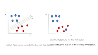
Multiple hyperplanes separatethe data from two classes
Selecting hyperplane for data with outlier
Here, we have one blue ball in the boundary of the red ball.
35.
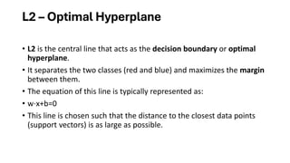
L2 – OptimalHyperplane
• L2 is the central line that acts as the decision boundary or optimal
hyperplane.
• It separates the two classes (red and blue) and maximizes the margin
between them.
• The equation of this line is typically represented as:
• w⋅x+b=0
• This line is chosen such that the distance to the closest data points
(support vectors) is as large as possible.
36.
L1 and L3– Margin Boundaries
•L1 and L3 are the margin lines on either side of the hyperplane L2.
•These lines pass through the support vectors, the closest points from each class to the
hyperplane.
•The distance between L1 and L3 is known as the margin, and SVM aims to maximize
this margin.
•The equations of these lines are:
•L1: w⋅x+b=+1
•L3: w⋅x+b=−1
37.
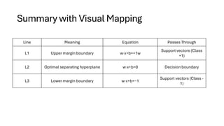
Summary with VisualMapping
Line Meaning Equation Passes Through
L1 Upper margin boundary w⋅x+b=+1w
Support vectors (Class
+1)
L2 Optimal separating hyperplane w⋅x+b=0 Decision boundary
L3 Lower margin boundary w⋅x+b=−1
Support vectors (Class -
1)
38.
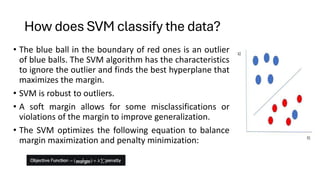
How does SVMclassify the data?
• The blue ball in the boundary of red ones is an outlier
of blue balls. The SVM algorithm has the characteristics
to ignore the outlier and finds the best hyperplane that
maximizes the margin.
• SVM is robust to outliers.
• A soft margin allows for some misclassifications or
violations of the margin to improve generalization.
• The SVM optimizes the following equation to balance
margin maximization and penalty minimization:
39.
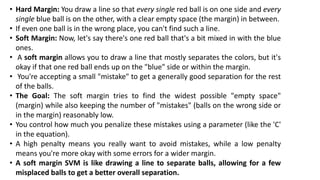
• Hard Margin:You draw a line so that every single red ball is on one side and every
single blue ball is on the other, with a clear empty space (the margin) in between.
• If even one ball is in the wrong place, you can't find such a line.
• Soft Margin: Now, let's say there's one red ball that's a bit mixed in with the blue
ones.
• A soft margin allows you to draw a line that mostly separates the colors, but it's
okay if that one red ball ends up on the "blue" side or within the margin.
• You're accepting a small "mistake" to get a generally good separation for the rest
of the balls.
• The Goal: The soft margin tries to find the widest possible "empty space"
(margin) while also keeping the number of "mistakes" (balls on the wrong side or
in the margin) reasonably low.
• You control how much you penalize these mistakes using a parameter (like the 'C'
in the equation).
• A high penalty means you really want to avoid mistakes, while a low penalty
means you're more okay with some errors for a wider margin.
• A soft margin SVM is like drawing a line to separate balls, allowing for a few
misplaced balls to get a better overall separation.
40.
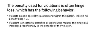
The penalty usedfor violations is often hinge
loss, which has the following behavior:
• If a data point is correctly classified and within the margin, there is no
penalty (loss = 0).
• If a point is incorrectly classified or violates the margin, the hinge loss
increases proportionally to the distance of the violation.
41.
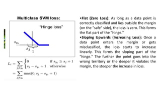
•Flat (Zero Loss):As long as a data point is
correctly classified and lies outside the margin
(on the "safe" side), the loss is zero. This forms
the flat part of the "hinge."
•Sloping Upwards (Increasing Loss): Once a
data point enters the margin or gets
misclassified, the loss starts to increase
linearly. This forms the sloping part of the
"hinge." The further the point goes into the
wrong territory or the deeper it violates the
margin, the steeper the increase in loss.
42.
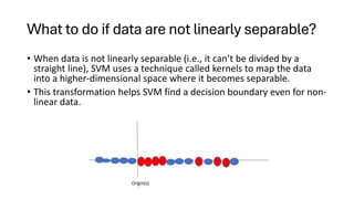
What to doif data are not linearly separable?
• When data is not linearly separable (i.e., it can’t be divided by a
straight line), SVM uses a technique called kernels to map the data
into a higher-dimensional space where it becomes separable.
• This transformation helps SVM find a decision boundary even for non-
linear data.
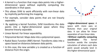
43.
• A kernelis a function that maps data points into a higher-
dimensional space without explicitly computing the
coordinates in that space.
• This allows SVM to work efficiently with non-linear data
by implicitly performing the mapping.
• For example, consider data points that are not linearly
separable.
• By applying a kernel function, SVM transforms the data
points into a higher-dimensional space where they
become linearly separable.
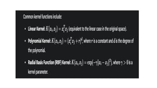
• Linear Kernel: For linear separability.
• Polynomial Kernel: Maps data into a polynomial space.
• Radial Basis Function (RBF) Kernel: Transforms data into a
space based on distances between data points.
• In this case, the new variable y is created as a function of
distance from the origin.
•Higher-dimensional space: A
space with more axes or
features than your original
data. It can allow for linear
separation of non-linear data.
•Without explicitly computing
coordinates: The kernel
function avoids the complex
calculation of where each data
point would actually land in
this higher-dimensional space
44.
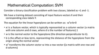
Mathematical Computation: SVM
Considera binary classification problem with two classes, labeled as +1 and -1.
We have a training dataset consisting of input feature vectors X and their
corresponding class labels Y.
The equation for the linear hyperplane can be written as: wTx+b=0
• xi is a feature vector, which is typically represented as a column vector (a matrix
with one column and d rows, where d is the number of features).1
• w is the normal vector to the hyperplane (the direction perpendicular to it).
• b is the offset or bias term, representing the distance of the hyperplane from the
origin along the normal vector
• wT transforms the column vector w into a row vector ((a matrix with one row and
d columns)
45.
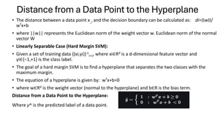
Distance from aData Point to the Hyperplane
• The distance between a data point x_i and the decision boundary can be calculated as: di=∣∣w∣∣/
wTx+b
• where ||w|| represents the Euclidean norm of the weight vector w. Euclidean norm of the normal
vector W
• Linearly Separable Case (Hard Margin SVM):
• Given a set of training data {(xi,yi)}n
i=1, where xi∈Rd is a d-dimensional feature vector and
yi∈{−1,+1} is the class label.
• The goal of a hard margin SVM is to find a hyperplane that separates the two classes with the
maximum margin.
• The equation of a hyperplane is given by: wTx+b=0
• where w∈Rd is the weight vector (normal to the hyperplane) and b∈R is the bias term.
Distance from a Data Point to the Hyperplane:
Where y^ is the predicted label of a data point.
46.
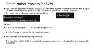
• For alinearly separable dataset, the goal is to find the hyperplane that maximizes the margin
between the two classes while ensuring that all data points are correctly classified.
• This leads to the following optimization problem:
Where:
• yi is the class label (+1 or -1) for each training instance.
• xi is the feature vector for the i-th training instance.
• M is the total number of training instances.
• The condition yi(wTxi+b)≥1 ensures that each data point is correctly classified and lies outside
the margin
Optimization Problem for SVM
47.
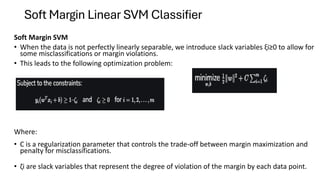
Soft Margin LinearSVM Classifier
Soft Margin SVM
• When the data is not perfectly linearly separable, we introduce slack variables ξi≥0 to allow for
some misclassifications or margin violations.
• This leads to the following optimization problem:
Where:
• C is a regularization parameter that controls the trade-off between margin maximization and
penalty for misclassifications.
• ζi are slack variables that represent the degree of violation of the margin by each data point.
48.
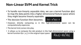
Non-Linear SVM andKernel Trick
• To handle non-linearly separable data, we use a kernel function ϕ(x)
to map the data points into a higher-dimensional feature space where
they might become linearly separable.
• The decision function then becomes:
• However, directly computing w in this high-dimensional space can be
computationally expensive.
• The kernel trick comes into play.
• It allows us to compute the dot product in the high-dimensional space using a
kernel function K(x i ,x j ) in the original input space:
50.
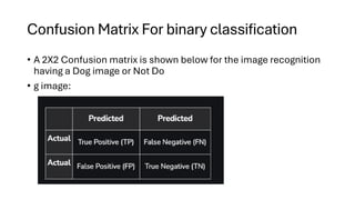
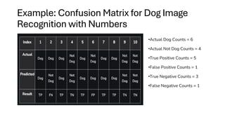
Confusion Matrix Forbinary classification
• A 2X2 Confusion matrix is shown below for the image recognition
having a Dog image or Not Do
• g image:
51.
• True Positive(TP): It is the total counts having both predicted and
actual values are Dog.
• True Negative (TN): It is the total counts having both predicted and
actual values are Not Dog.
• False Positive (FP): It is the total counts having prediction is Dog while
actually Not Dog.
• False Negative (FN): It is the total counts having prediction is Not Dog
while actually, it is Dog.
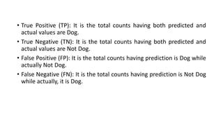
52.
Example: Confusion Matrixfor Dog Image
Recognition with Numbers
•Actual Dog Counts = 6
•Actual Not Dog Counts = 4
•True Positive Counts = 5
•False Positive Counts = 1
•True Negative Counts = 3
•False Negative Counts = 1
Performance metrics
• Performancemetrics are quantitative measures used to evaluate the
effectiveness and quality of a machine learning model's predictions
on a given dataset.
• They provide insights into how well the model is achieving its
intended task, such as classification or regression.
55.
Precision
• Precision refersto how consistently a tool or process can produce similar results
under the same conditions.
• It is about repeatability and reliability; not necessarily how close these results
are to the true or intended value.
Repeatability – Same person, same tool, same conditions, short time.
E.g., You weigh an apple on your kitchen scale five times in a row, and it shows 150
grams each time. Same person, same scale, same conditions = good repeatability!
Reproducibility – Different people, different tools, different times.
E.g., Your friend weighs the same apple using their own kitchen scale at their house
a day later, and it also reads about 150 grams. Different person, different scale,
different time = good reproducibility!
56.
Precision Formula
•True Positives(TP): The number of instances
correctly predicted as positive.
•False Positives (FP): The number of instances
incorrectly predicted as positive (they were actually
negative).
High precision means the model is good at not labeling negative samples as positive. It has a low false positive
rate.
Example :
Model predicted 10 spam emails, 7 were spam.
7 / (7 + 3) = 0.7
57.
Recall
• Recall measuresthe ability of a model to correctly identify all actual positive cases.
It is the proportion of true positives (TP) out of all actual positives (TP + FN).
• Example : Suppose you're building a model to detect spam emails.
• There are 100 actual spam emails (positive cases).
• Your model correctly identifies 80 of them as spam → TP = 80
• It misses 20 spam emails, marking them as not spam → FN = 20
Recall=80/(80+20)=80/100=0.80
High Recall = Model catches most of the actual positives (few false negatives).
Low Recall = Model is missing many real positive cases.
58.
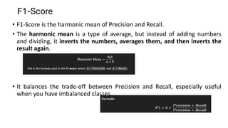
F1-Score
• F1-Score isthe harmonic mean of Precision and Recall.
• The harmonic mean is a type of average, but instead of adding numbers
and dividing, it inverts the numbers, averages them, and then inverts the
result again.
• It balances the trade-off between Precision and Recall, especially useful
when you have imbalanced classes.
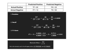
ROC-AUC (Receiver OperatingCharacteristic –
Area Under the Curve)
ROC-AUC measures a model's ability to
distinguish between classes.
•The ROC curve plots True Positive
Rate (Recall) vs. False Positive Rate
(FPR) at various threshold settings.
•AUC is the area under this curve,
ranging from 0 to 1.
•False Positive (FP): Instances that
were incorrectly predicted as positive
but belong to the negative class.
•True Negative (TN): Instances that
were correctly predicted as negative. The ROC curve is generated by plotting the TPR against the
FPR at various threshold settings for your classifier.
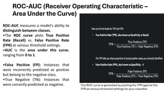
61.
Predicted Positive PredictedNegative
Actual Positive TP = 80 FN = 20
Actual Negative FP = 10 TN = 90
•False Positive Rate (FPR) =
10/10+90=10/100=0.1
•True Positive Rate (Recall):
Recall=TPTP+FN=80/80+20=80/100=0.8
•AUC = 1.0 → Perfect model
•AUC = 0.5 → No better than random guessing
•AUC < 0.5 → Worse than random (flawed model)
•False Positive Rate (FPR): 0.1
•True Positive Rate (Recall):0.8
•AUC is the area under this curve, ranging from 0 to 1.
62.
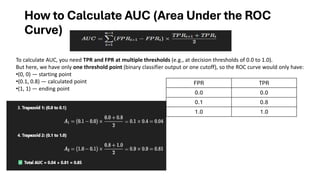
How to CalculateAUC (Area Under the ROC
Curve)
To calculate AUC, you need TPR and FPR at multiple thresholds (e.g., at decision thresholds of 0.0 to 1.0).
But here, we have only one threshold point (binary classifier output or one cutoff), so the ROC curve would only have:
•(0, 0) — starting point
•(0.1, 0.8) — calculated point
•(1, 1) — ending point
FPR TPR
0.0 0.0
0.1 0.8
1.0 1.0
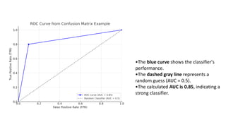
63.
•The blue curveshows the classifier's
performance.
•The dashed gray line represents a
random guess (AUC = 0.5).
•The calculated AUC is 0.85, indicating a
strong classifier.
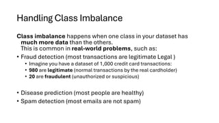
Handling Class Imbalance
Classimbalance happens when one class in your dataset has
much more data than the others.
This is common in real-world problems, such as:
• Fraud detection (most transactions are legitimate Legal )
• Imagine you have a dataset of 1,000 credit card transactions:
• 980 are legitimate (normal transactions by the real cardholder)
• 20 are fraudulent (unauthorized or suspicious)
• Disease prediction (most people are healthy)
• Spam detection (most emails are not spam)
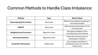
67.
Common Methods toHandle Class Imbalance:
Method Type What it Does
Resampling (Over/Under) Data-level
Balance the dataset by adding or
removing samples
SMOTE Data-level
Adds synthetic examples for the
minority class
Weighted Loss Functions Algorithm-level
Penalizes mistakes on the
minority class more heavily
Anomaly Detection Algorithm-level
Treats the minority class as
anomalies or outliers
Ensemble Techniques Model-level
Use multiple classifiers or
boosting to focus on minority
class errors
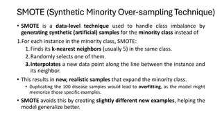
68.
SMOTE (Synthetic MinorityOver-sampling Technique)
• SMOTE is a data-level technique used to handle class imbalance by
generating synthetic (artificial) samples for the minority class instead of
1.For each instance in the minority class, SMOTE:
1.Finds its k-nearest neighbors (usually 5) in the same class.
2.Randomly selects one of them.
3.Interpolates a new data point along the line between the instance and
its neighbor.
• This results in new, realistic samples that expand the minority class.
• Duplicating the 100 disease samples would lead to overfitting, as the model might
memorize those specific examples.
• SMOTE avoids this by creating slightly different new examples, helping the
model generalize better.
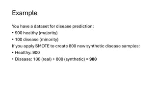
69.
Example
You have adataset for disease prediction:
• 900 healthy (majority)
• 100 disease (minority)
If you apply SMOTE to create 800 new synthetic disease samples:
• Healthy: 900
• Disease: 100 (real) + 800 (synthetic) = 900
70.
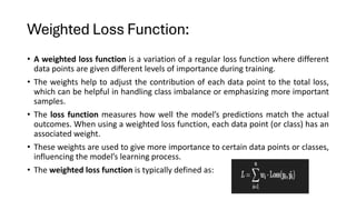
Weighted Loss Function:
•A weighted loss function is a variation of a regular loss function where different
data points are given different levels of importance during training.
• The weights help to adjust the contribution of each data point to the total loss,
which can be helpful in handling class imbalance or emphasizing more important
samples.
• The loss function measures how well the model’s predictions match the actual
outcomes. When using a weighted loss function, each data point (or class) has an
associated weight.
• These weights are used to give more importance to certain data points or classes,
influencing the model’s learning process.
• The weighted loss function is typically defined as:
71.
Where:
• wi isthe weight assigned to the i-th data point (or class).
• Loss(yi,yi^)) is the loss
• yi is the true label for the i-th data point.
• yi^ is the predicted value for the i-th data point.
72.
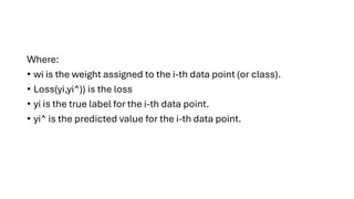
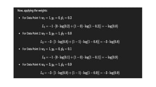
Example: Weighted Lossin Classification
• Consider a binary classification problem where we want to classify data into two classes: Class 0
and Class 1.
• If we have an imbalanced dataset where Class 1 is much less frequent than Class 0,
• we can assign a higher weight to Class 1 to ensure the model focuses more on correctly
classifying the rare class
Scenario:
Let’s say we have the following data points:
• Data Point 1: True label y1=0, predicted probability p1^=0.2
• Data Point 2: True label y2=1, predicted probability p2^=0.8
• Data Point 3: True label y3=0, predicted probability p3^=0.1
• Data Point 4: True label y4=1, predicted probability p4^=0.9
73.
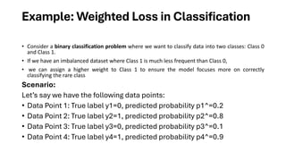
• Assume thatClass 1 (the positive class) is underrepresented. We
assign a weight of 3 to Class 1
• weight of 1 to Class 0 to penalize errors in the minority class
more.
Weighted Cross-Entropy Loss:
• The formula for binary cross-entropy loss is:
75.
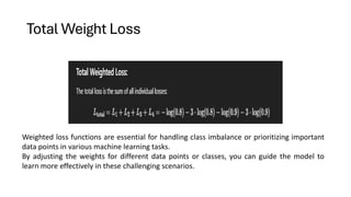
Total Weight Loss
Weightedloss functions are essential for handling class imbalance or prioritizing important
data points in various machine learning tasks.
By adjusting the weights for different data points or classes, you can guide the model to
learn more effectively in these challenging scenarios.

![• Here xi is the I th observation of X, wi=[w1,w2,w3,⋯,wm] is the
weights or Coefficient, and b is the bias term also known as intercept.
simply this can be represented as the dot product of weight a
• z=w⋅X+b bias. Which is a linear regression.
Linear Function
• Combine inputs linearly:
• z=w⋅X+b
• Where:
• w = weights
• X = input features
• b = bias (intercept)](https://image.slidesharecdn.com/module-6-250703080633-4f71971e/85/Module-6-pdf-Machine-Learning-Types-and-examples-14-320.jpg)
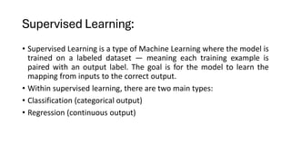
![Example
Scenario: Predicting if a student passes
• Study hours = 4
• Sleep hours = 7
• Weights: w=[0.6,0.2],b=−2
• z=w⋅X+b
• z=0.6(4)+0.2(7)−2=1.8
• p=σ(1.8)≈0.858p
• Prediction: Student passes (since 0.858 > 0.5)](https://image.slidesharecdn.com/module-6-250703080633-4f71971e/85/Module-6-pdf-Machine-Learning-Types-and-examples-17-320.jpg)
![Summary
•Logistic Regression → for binary classification
•Uses sigmoid function to map output to [0, 1]
•Interprets result as probability
•Linear model applied to log-odds](https://image.slidesharecdn.com/module-6-250703080633-4f71971e/85/Module-6-pdf-Machine-Learning-Types-and-examples-18-320.jpg)
![import pandas as pd
from sklearn.model_selection import train_test_split
from sklearn.tree import DecisionTreeClassifier
from sklearn.metrics import accuracy_score,
classification_report, confusion_matrix
from sklearn import preprocessing
import matplotlib.pyplot as plt
from sklearn import tree
# Sample Loan Approval Data (replace with your actual
data)
data = {
'Credit_Score': ['Poor', 'Fair', 'Good', 'Excellent',
'Good', 'Fair', 'Excellent', 'Poor', 'Good', 'Excellent'],
'Income': [25000, 40000, 60000, 80000, 55000,
35000, 90000, 30000, 70000, 100000],
'Debt_to_Income': [0.5, 0.4, 0.2, 0.1, 0.3, 0.6, 0.15,
0.55, 0.25, 0.05],
'Loan_Amount': [5000, 15000, 25000, 40000, 20000,
10000, 50000, 8000, 30000, 60000],
'Loan_Term': ['Short', 'Medium', 'Long', 'Short',
'Medium', 'Short', 'Long', 'Short', 'Medium', 'Long'],
'Property_Value': [80000, 150000, 300000, 500000,
250000, 120000, 600000, 100000, 350000, 750000],
'Loan_Approved': ['No', 'No', 'Yes', 'Yes', 'Yes', 'No',
'Yes', 'No', 'Yes', 'Yes']
}
df = pd.DataFrame(data)
# Convert categorical features to numerical using Label
Encoding
label_encoder = preprocessing.LabelEncoder()
df['Credit_Score'] =
label_encoder.fit_transform(df['Credit_Score'])
df['Loan_Term'] =
label_encoder.fit_transform(df['Loan_Term'])
df['Loan_Approved'] =
label_encoder.fit_transform(df['Loan_Approved']) #
Yes: 1, No: 0
# Separate features (X) and target (y)
X = df.drop('Loan_Approved', axis=1)
y = df['Loan_Approved']
# Split data into training and testing sets
X_train, X_test, y_train, y_test = train_test_split(X, y,
test_size=0.3, random_state=42)
# Initialize and train the Decision Tree Classifier
dt_classifier =
DecisionTreeClassifier(random_state=42)
dt_classifier.fit(X_train, y_train)
# Make predictions on the test set
y_pred = dt_classifier.predict(X_test)
# Evaluate the model
accuracy = accuracy_score(y_test, y_pred)
print(f"Accuracy: {accuracy:.2f}")
print("nClassification Report:")
print(classification_report(y_test, y_pred))
print("nConfusion Matrix:")
print(confusion_matrix(y_test, y_pred))
# Visualize the Decision Tree (requires graphviz to be
installed)
plt.figure(figsize=(15, 10))
tree.plot_tree(dt_classifier,
feature_names=X.columns, class_names=['No', 'Yes'],
filled=True)
plt.title("Decision Tree for Loan Approval")
plt.show()](https://image.slidesharecdn.com/module-6-250703080633-4f71971e/85/Module-6-pdf-Machine-Learning-Types-and-examples-29-320.jpg)


![Unit-3-Part-1 [Autosaved].ppt](https://cdn.slidesharecdn.com/ss_thumbnails/unit-3-part-1autosaved-230216062941-16596250-thumbnail.jpg?width=640&height=640&fit=bounds)


