MODULE-1.pptx machine learning note for 6th sem vtu
1.
MODULE-1
• Introduction: Needfor Machine Learning, Machine Learning Explained,
Machine Learning in Relation to other Fields, Types of Machine Learning,
Challenges of Machine Learning, Machine Learning Process, Machine
Learning Applications.
• Understanding Data – 1: Introduction, Big Data Analysis Framework,
Descriptive Statistics, Univariate Data Analysis and Visualization.
• https://chatgpt.com/share/67aadbaa-5edc-8009-9ac6-325bee59d0d4
2.
Need for MachineLearning
• If humans can give ability of thinking hearing, recognizing and making decisions
to a machine, what is the need of giving that power to a machine?
• From a human perspective, the need for machine learning (ML) comes from our
desire to make life easier, solve complex problems, and push the boundaries of
what we can achieve. However, this also raises deeper questions about dependence
and control.
• Handling Complexity Beyond Human Capability
• Automating the Mundane,
• Freeing the Human Mind
• Enhancing Human Decision-Making
• Personalization: Making Life More Efficient
• The Human Desire to Innovate
3.
• Business organizationsuse huge amount of data for their daily activities.
Earlier, the full potential of this data was not utilized due to two reasons.
• One reason was data being scattered across different archive systems and
organizations not being able to integrate these sources fully.
• Secondly, the lack of awareness about software tools that could help to
unearth the useful information from data.
• Not anymore! Business organizations have now started to use the latest
technology, machine learning, for this purpose.
Machine learning has become so popular because of three reasons:
• 1. High volume of available data to manage: Big companies such as
Facebook, Twitter, and YouTube generate huge amount of data that grows at
a phenomenal rate. It is estimated that the data approximately gets doubled
every year.
4.
• Second reasonis that the cost of storage has reduced. The hardware cost has
also dropped. Therefore, it is easier now to capture, process, store, distribute,
and transmit the digital information.
• Third reason for popularity of machine learning is the availability of complex
algorithms now. Especially with the advent of deep learning, many algorithms
are available for machine learning.
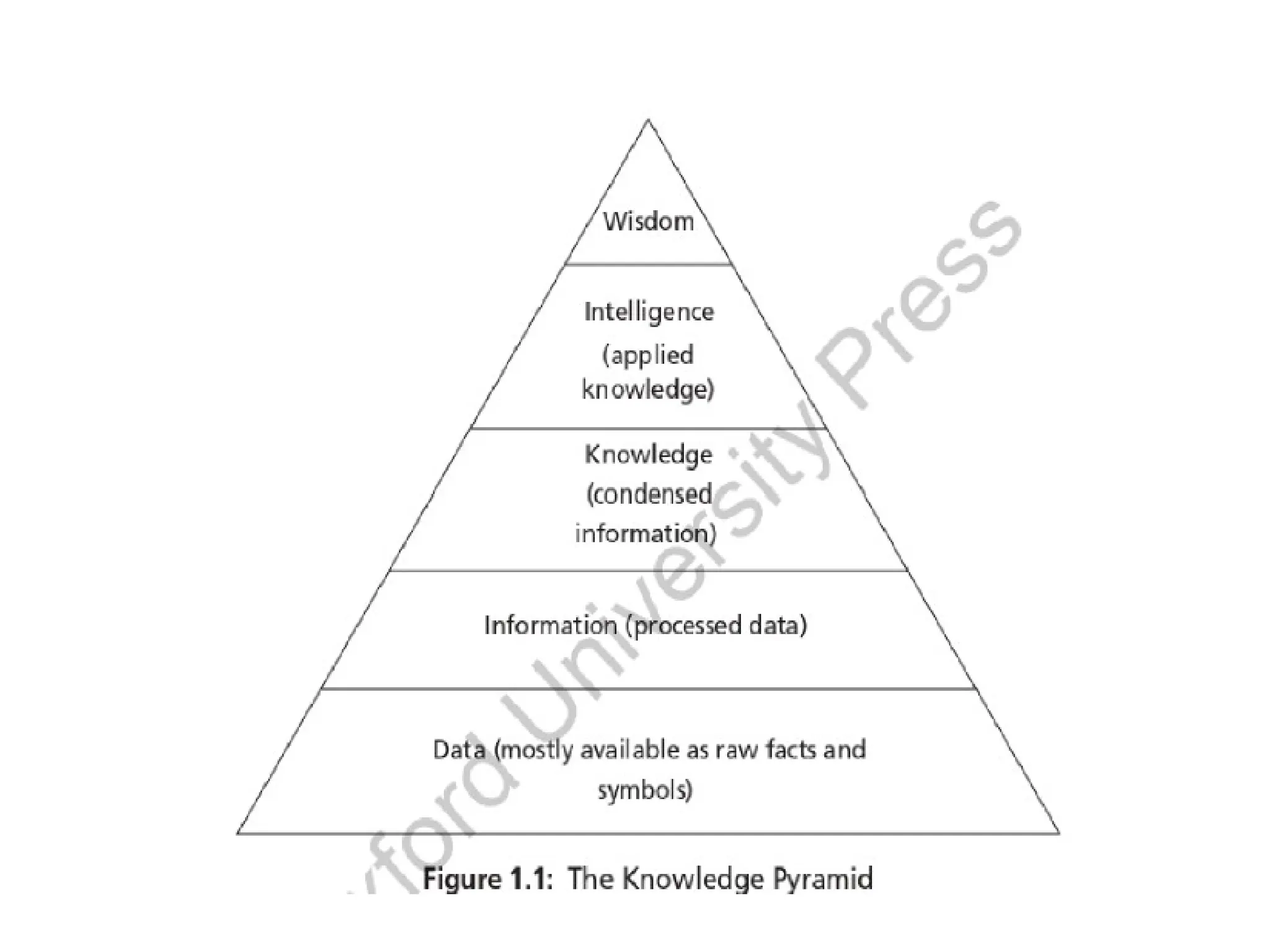
• Before starting the machine learning journey, let us establish these terms - data,
information, knowledge, intelligence, and wisdom. A knowledge pyramid is
shown in Figure 1.1.
• What is data? All facts are data. Data can be numbers or text that can be
processed by a computer. Today, organizations are accumulating vast and
growing amounts of data with data sources such as flat files, databases, or data
warehouses in different storage formats.
6.
• Processed datais called information. This includes patterns, associations,
or relationships among data, Condensed information is called knowledge.
• Similarly, knowledge is not useful unless it is put into action. Intelligence
is the applied knowledge for actions. An actionable form of knowledge is
called intelligence. Computer systems have been successful till this stage.
The ultimate objective of knowledge pyramid is wisdom that represents the
maturity of mind that is, so far, exhibited only by humans.
7.
Introduction to MachineLearning
• Machine learning is an important sub-branch of Artificial Intelligence (AI). A
frequently quoted definition of machine learning was by Arthur Samuel, one of the
pioneers of Artificial Intelligence. He stated that “Machine learning is the field of
study that gives the computers ability to learn without being explicitly programmed.”
• The idea of developing intelligent systems by using logic and reasoning by
converting an expert's knowledge into a set of rules and programs is called an expert
system.
• The above approach was impractical in many domains as programs still depended on
human expertise and hence did not truly exhibit intelligence. Then, the momentum
shifted to machine learning in the form of data driven systems. The focus of Al is to
develop intelligent systems by using data-driven approach, where data is used as an
input to develop intelligent models.
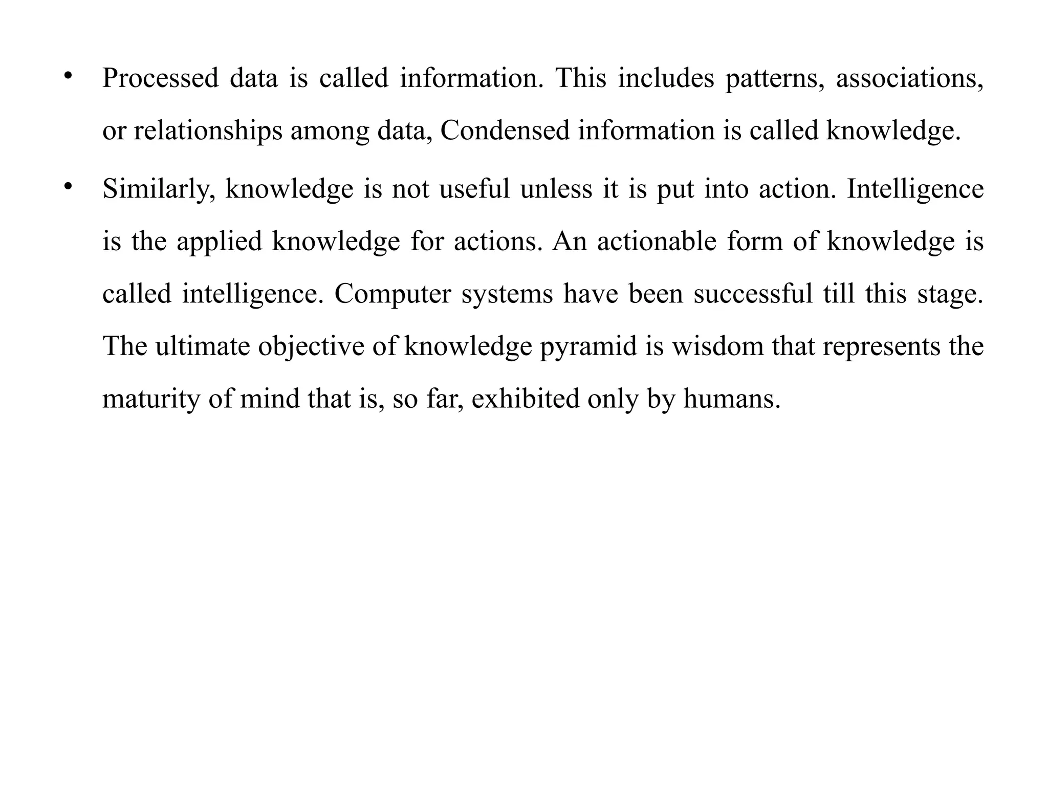
8.
• The modelscan then be used to predict new inputs. Thus, the aim of machine
learning is to learn a model or set of rules from the given dataset automatically
so that it can predict the unknown data correctly.
• As humans take decisions based on an experience, computers make models
based on extracted patterns in the input data and then use these data-filled
models for prediction and to take decisions. For computers, the learnt model is
equivalent to human experience. This is shown in Figure 1.2.
9.
• In statisticallearning, the relationship between the input x and output y is modeled
as a function in the form y = f(x). Here, f£ is the learning function that maps the
input x to output y. Learning of function f is the crucial aspect of forming a model
in statistical learning, In machine learning, this is simply called mapping of input
to output.
• The learning program summarizes the raw data in a model. Formally stated, a
model is an explicit description of patterns within the data in the form of:
1. Mathematical equation
2. Relational diagrams like trees/graphs
3. Logical if/else rules, or
4. Groupings called clusters
• In summary, a model can be a formula, procedure or representation that can
generate data decisions. The difference between pattern and model is that the
former is local and applicable only to certain attributes but the latter is global and
fits the entire dataset.
10.
• For example,a model can be helpful to examine whether a given email is spam or
not. The point is that the model is generated automatically from the given data.
• Tom Mitchell's definition of machine learning states that, “A computer program is
said to learn from experience E, with respect to task T and some performance
measure P, if its performance on T measured by P improves with experience E.” The
important components of this definition are experience E, task T, and performance
measure P.
• For example, the task T could be detecting an object in an image. The machine can
gain the knowledge of object using training dataset of thousands of images. This is
called experience E. So, the focus is to use this experience E for this task-of object
detection T.
• The ability of the system to detect the object is measured by performance measures
like precision and recall. Based on the performance measures, course correction can
be done to improve the performance of the system.
11.
• Models ofcomputer systems are equivalent to human experience. Experience is
based on data. Humans gain experience by various means. But, in systems,
experience is gathered by these steps:
1. Collection of data
2. Once data is gathered, abstract concepts are formed out of that data. Abstraction
is use to generate concepts. This is equivalent to humans’ idea of objects, for
example, we have some idea about how an elephant looks like.
3. Generalization converts the abstraction into an actionable form of intelligence. It
can be viewed as ordering of all possible concepts. So, generalization involves
ranking of concepts, inferencing from them and formation of heuristics, an
actionable aspect of intelligence. Heuristics are educated guesses for all tasks.
12.
For example, ifone runs or encounters a danger, it is the resultant of human
experience or his heuristics formation. In machines, it happens the same way.
4. Heuristics normally works! But, occasionally, it may fail too. It is not the fault of
heuristics as it is just a ‘rule of thumb’. The course correction is done by taking
evaluation measures. Evaluation checks the thoroughness of the models and to-
do course correction, if necessary, to generate better formulations.
13.
MACHINE LEARNING INRELATION TO OTHER
FIELDS
Machine learning uses the concepts of Artificial Intelligence, Data Science, and
Statistics primarily. It is the resultant of combined ideas of diverse fields.
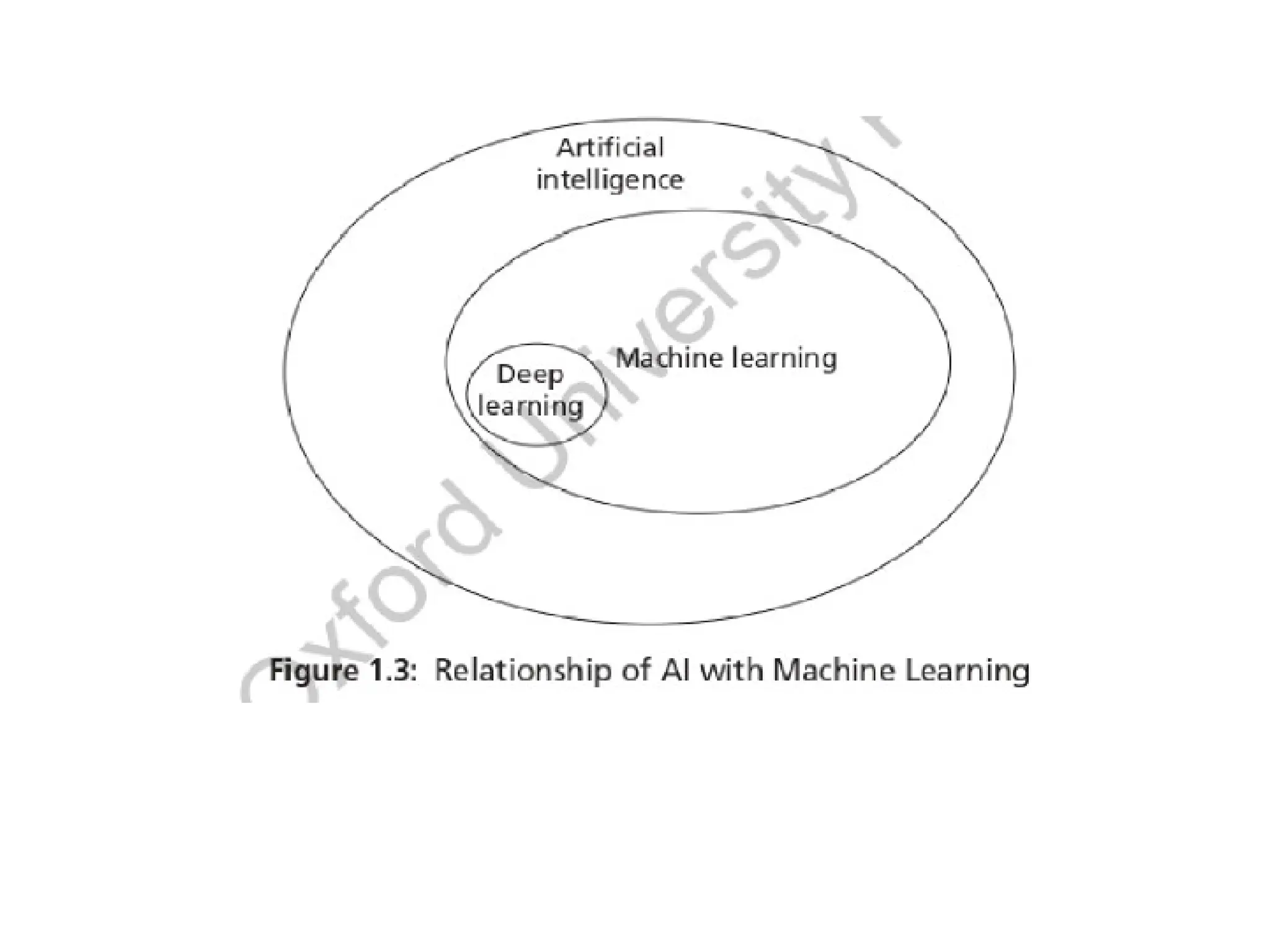
Machine Learning and Artificial Intelligence
• The aim of Al is to develop intelligent agents. An agent can be a robot,
humans, or any autonomous systems. Initially, the idea of Al was ambitious,
that is, to develop intelligent systems like human beings. The focus was on
logic and logical inferences.
• Machine learning is the subbranch of Al, whose aim is to extract the
patterns for prediction. It is a broad field that includes learning from
examples and other areas like reinforcement learning. The relationship
of AI and machine learning is shown in Figure 1.3.
15.
• Deep learningis a sub branch of machine learning. In deep learning, the models
are constructed using neural network technology. Neural networks are based on
the human neuron models. Many neurons form a network connected with the
activation functions that trigger further neurons to perform tasks.
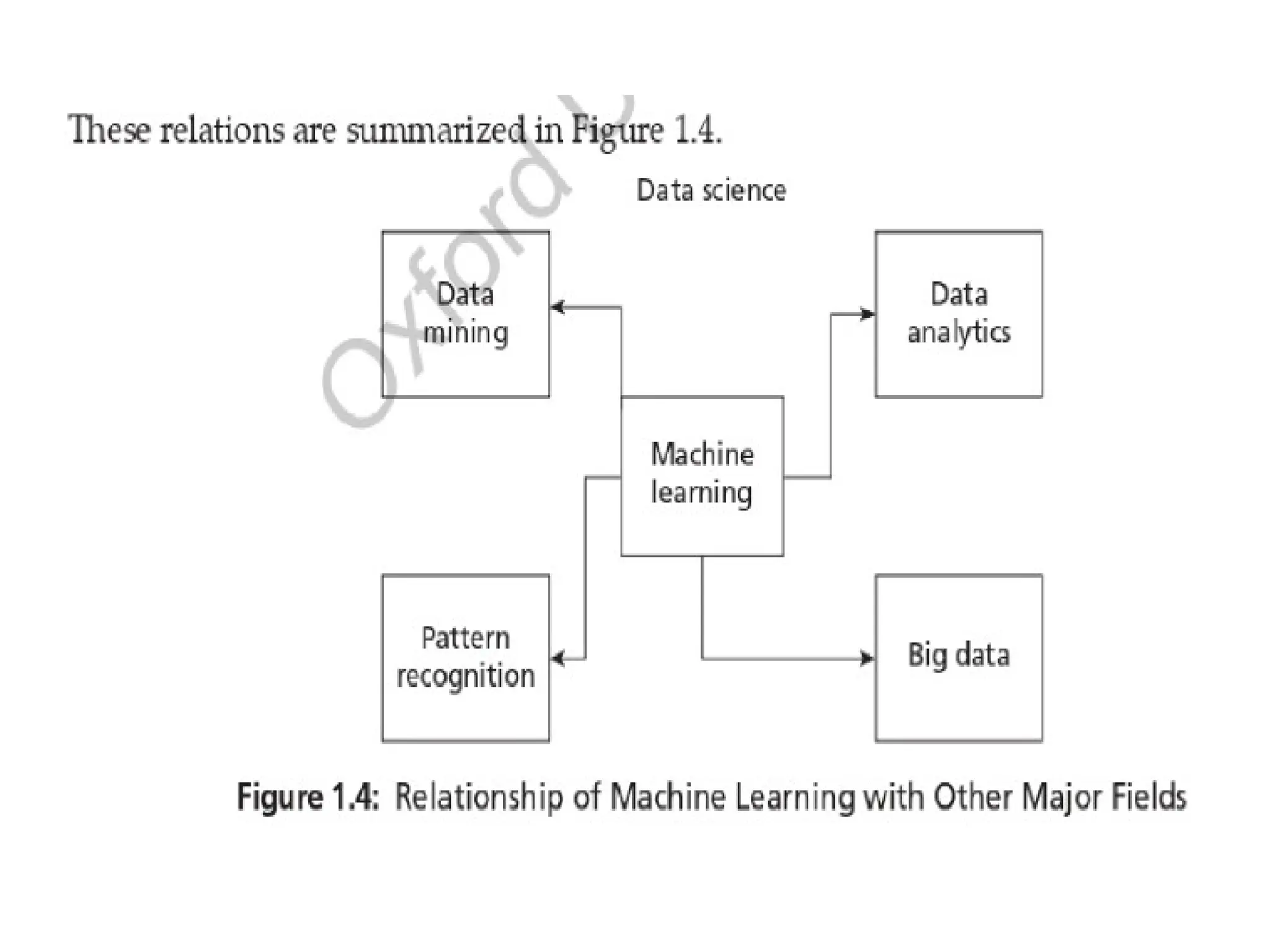
Machine Learning, Data Science, Data Mining, and Data Analytics
• Machine learning starts with data. Therefore, data science and machine
learning are interlinked. Machine learning is a branch of data science. Data
science deals with gathering o data for analysis.
– It is a broad field that includes: Big Data Data science concerns about
collection of data. Big data is a field of data science that deals with data’s
following characteristics:
– 1. Volume: Huge amount of data is generated by big companies like
Facebook, Twitter, YouTube.
16.
• 2. Variety:Data is available in variety of forms like images, videos, and in
different formats.
• 3. Velocity: It refers to the speed at which the data is generated and processed.
• Data Mining: Nowadays, many consider that data mining and machine learning are
same. There is no-difference between these fields except that data mining aims to
extract the hidden patterns that are present in the data, whereas, machine learning
aims to use it for prediction.
• Data Analytics Another branch of data science is data analytics. It aims to extract
useful knowledge from crude data. There are different types of analytics. Predictive
data analytics is used for making predictions. Machine learning is closely related to
this branch of analytics and shares almost all algorithms.
• Pattern Recognition It is an engineering, field. It uses machine learning algorithms
to extract the features for pattern analysis and pattern classification. One can view
pattern recognition as a specific application of machine learning.
18.
Machine Learning andStatistics
• Statistics is a branch of mathematics that has a solid theoretical foundation
regarding statistical learning. Like machine learning (ML), it can learn from
data. But the difference between statistics and ML is that statistical methods
look for regularity in data called patterns. Initially, statistics sets a hypothesis
and performs experiments to verify and validate the hypothesis in order to find
relationships among data.
• Machine learning, comparatively, has less assumptions and requires less
statistical knowledge. But, it often requires interaction with various tools to
automate the process of learning.
19.
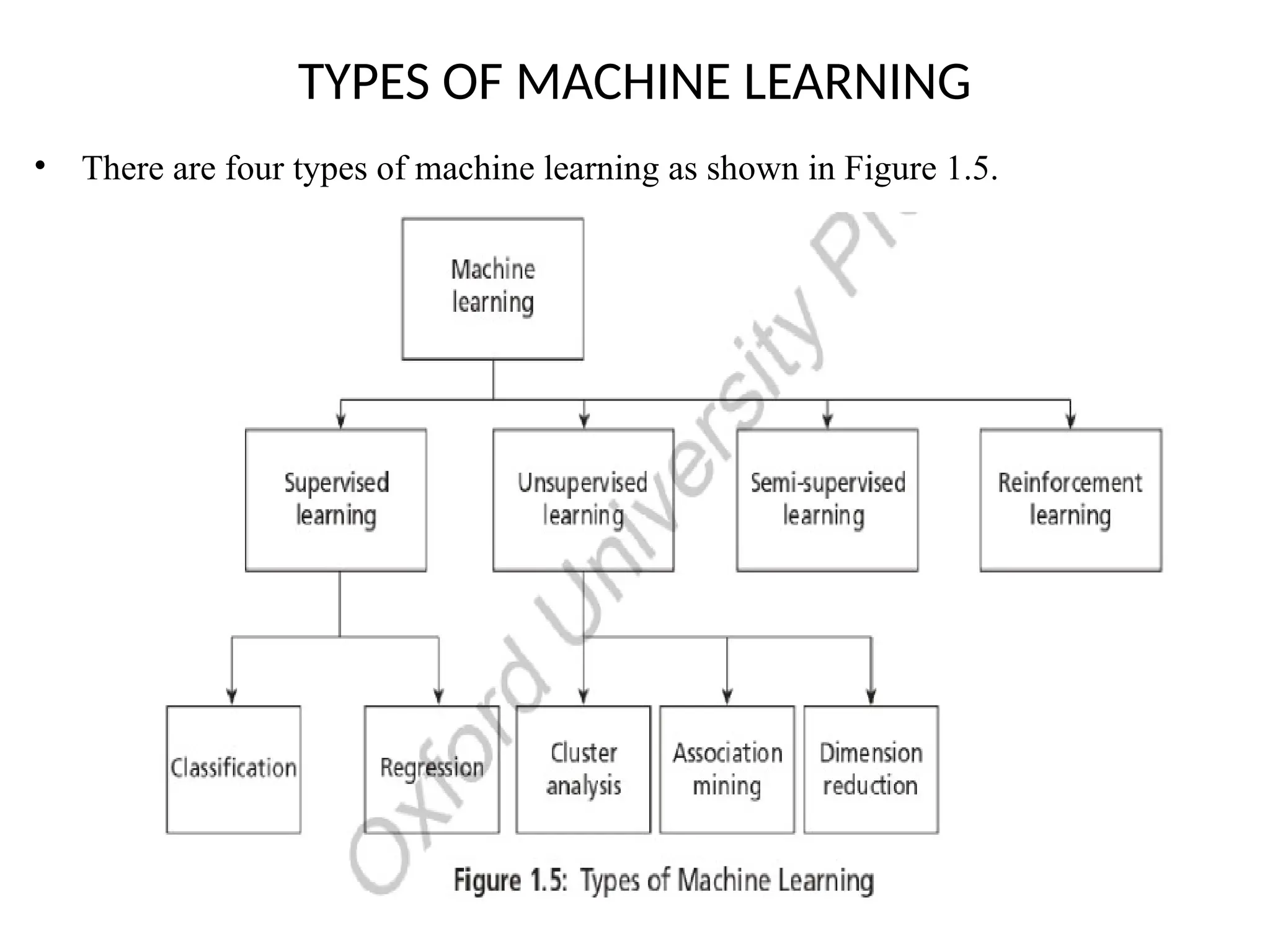
TYPES OF MACHINELEARNING
• There are four types of machine learning as shown in Figure 1.5.
20.
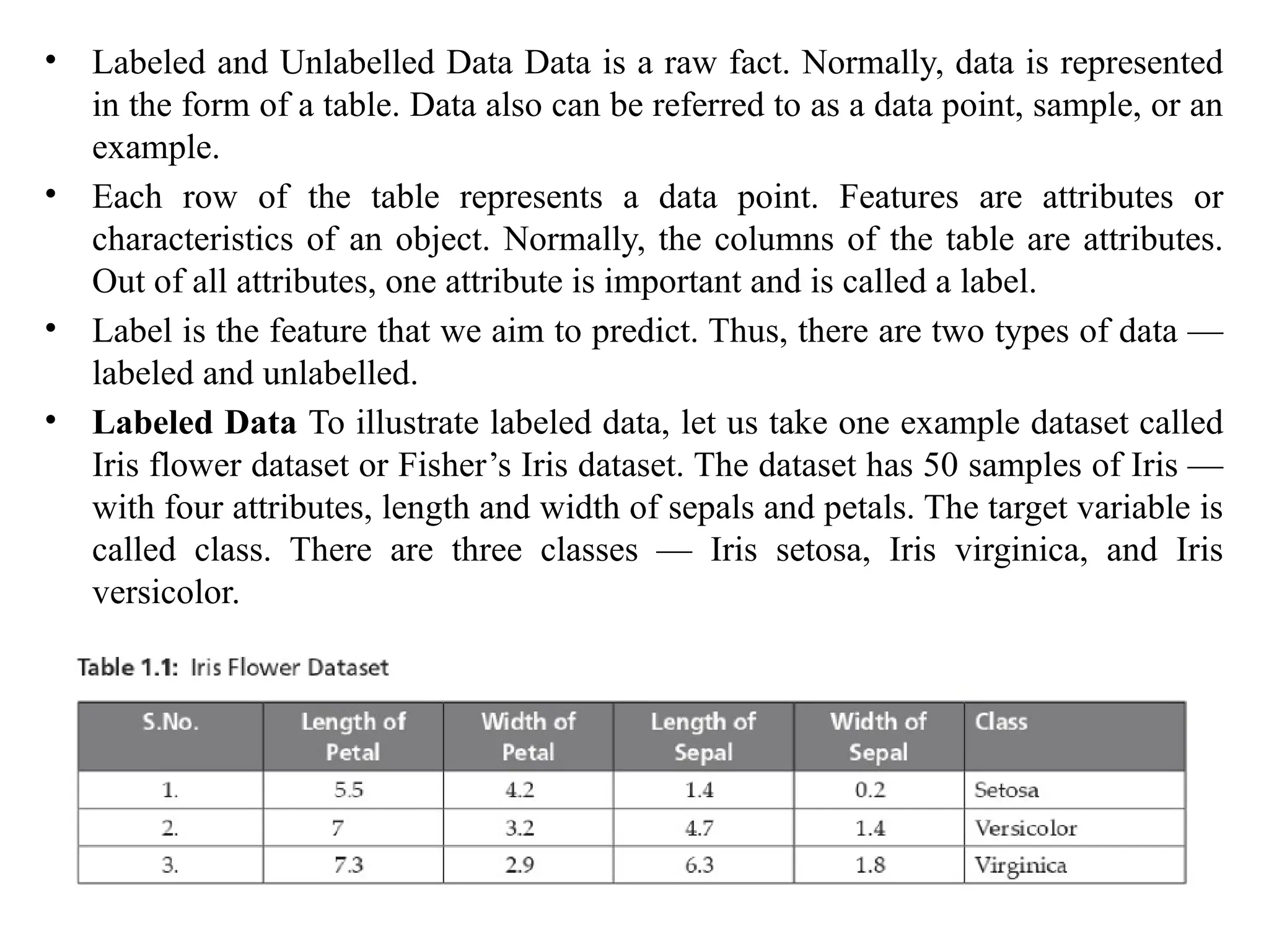
• Labeled andUnlabelled Data Data is a raw fact. Normally, data is represented
in the form of a table. Data also can be referred to as a data point, sample, or an
example.
• Each row of the table represents a data point. Features are attributes or
characteristics of an object. Normally, the columns of the table are attributes.
Out of all attributes, one attribute is important and is called a label.
• Label is the feature that we aim to predict. Thus, there are two types of data —
labeled and unlabelled.
• Labeled Data To illustrate labeled data, let us take one example dataset called
Iris flower dataset or Fisher’s Iris dataset. The dataset has 50 samples of Iris —
with four attributes, length and width of sepals and petals. The target variable is
called class. There are three classes — Iris setosa, Iris virginica, and Iris
versicolor.
21.
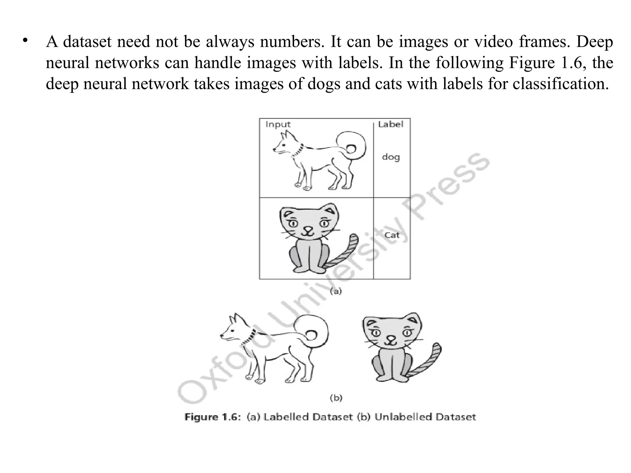
• A datasetneed not be always numbers. It can be images or video frames. Deep
neural networks can handle images with labels. In the following Figure 1.6, the
deep neural network takes images of dogs and cats with labels for classification.
22.
• Supervised algorithmsuse labeled dataset. As the name suggests, there is a
supervisor or teacher component in supervised learning. A supervisor provides
labeled data so that the model is constructed and generates test data.
• It happens in two stages training stage and testing stage
• Supervised learning has two methods:
– 1. Classification
– 2. Regression
Classification
• Classification is a supervised learning method. The input attributes of the
classification algorithms are called independent variables. The target attribute
is called label or dependent variable.
23.
• The relationshipbetween the input and target variable is represented in the form
of a structure which is called a classification model. So, the focus of
classification is to predict the ‘label’ that is in a discrete form (a value from the
set of finite values).
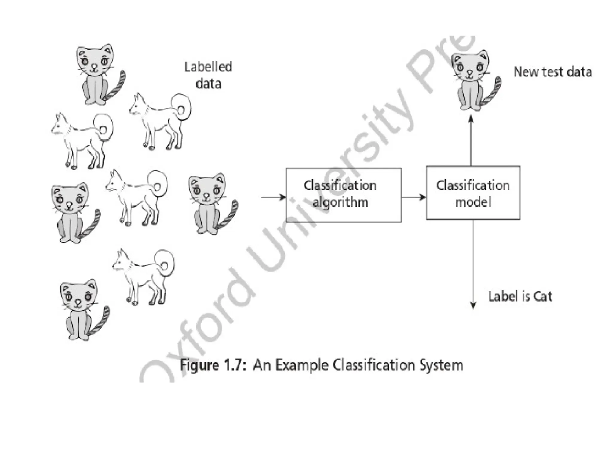
• An example is shown in Figure 1.7 where a classification algorithm takes a set
of labelled data images such as dogs and cats to construct a model that can later
be used to classify an unknown test image data.
• In classification, learning takes place in two stages. During the first stage, called
training stage, the learning algorithm takes a labelled dataset and starts learning.
After the training set, samples are processed and the model is generated. In the
second stage, the constructed model is tested with test or unknown sample and
assigned a label. This is the classification process.
25.
• Some ofthe key algorithms of classification are:
– Decision Tree
– Random Forest
– Support Vector Machines
– Naive Bayes
– Artificial Neural Network and Deep Learning networks like CNN
Regression
• Regression models, unlike classification algorithms, predict continuous
variables like price.
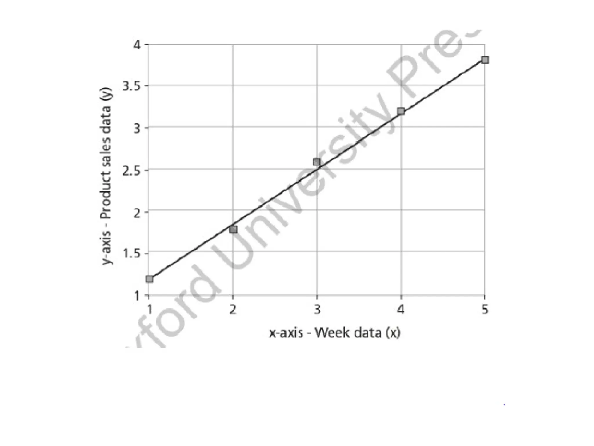
• In other words, it is a number. A fitted regression model is shown in Figure 1.8
for a dataset that represent weeks input x and product sales y.
27.
• The regressionmodel takes input x and generates a model in the form of a fitted
line of the form y = f(x). Here, x is the independent variable that may be one or
more attributes and y is the dependent variable.
• In Figure 1.8, linear regression takes the training set and tries to fit it with a line
— product sales = 0.66 x Week + 0.54. Here, 0.66 and 0.54 are all regression
coefficients that are learnt from data.
• The advantage of this model is that prediction for product sales (y) can be made
for unknown week data (x). For example, the prediction for unknown eighth
week can be made by substituting x as 8 in that regression formula to get y.
28.
Unsupervised Learning
• Thesecond kind of learning is by self-instruction. As the name suggests, there
are no supervisor or teacher components. In the absence of a supervisor or
teacher, self-instruction is the most common kind of learning process. This
process of selt-instruction is based on the concept of trial and error.
• Here, the program is supplied with objects, but no labels are defined. The
algorithm itself observes the examples and recognizes patterns based on the
principles of grouping. Grouping is done in ways that similar objects form the
same group.
• Cluster analysis and Dimensional reduction algorithms are examples of
unsupervised algorithms.
• .
29.
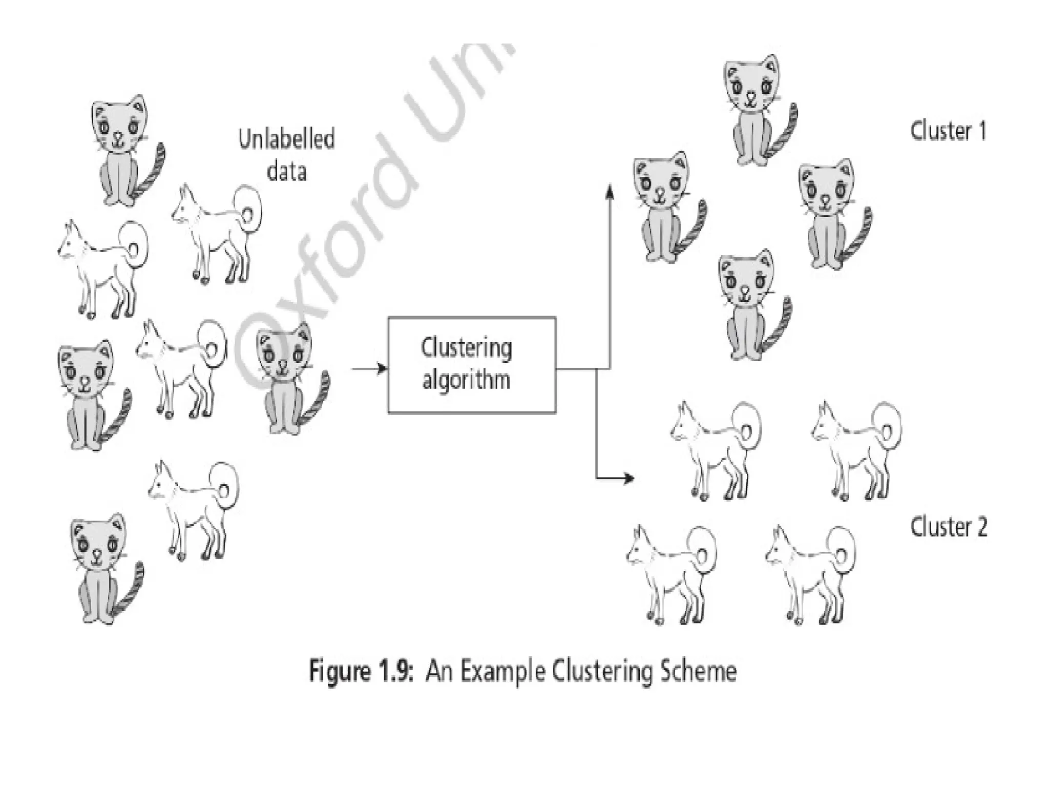
Cluster Analysis
• Clusteranalysis is an example of unsupervised learning. It aims to group objects
into disjoint clusters or groups.
• Cluster analysis clusters objects based on its attributes. All the data objects of
the partitions are similar in some aspect and vary from the data objects in the
other partitions significantly.
• Some of the examples of clustering processes are — segmentation of a region of
interest in an image, detection of abnormal growth in a medical image, and
determining clusters of signatures in a gene database.
• An example of clustering scheme is shown in Figure 1.9 where the clustering
algorithm takes a set of dogs and cats images and groups it as two clusters-dogs
and cats. It can be observed that the samples belonging to a cluster are similar
and samples are different radically across clusters.
31.
• Some ofthe key clustering algorithms are:
• k-means algorithm
• Hierarchical algorithms
Dimensionality Reduction
• Dimensionality reduction algorithms are examples of unsupervised algorithms.
It takes a higher dimension data as input and outputs the data in lower
dimension by taking advantage of the variance of the data.
• It is a task of reducing the dataset with few features without losing the
generality.
32.
Semi-supervised Learning
• Thereare circumstances where the dataset has a huge collection of unlabelled
data and some labelled data. Labelling is a costly process and difficult to.pertorm
by the humans. Semi-supervised algorithms use unlabelled data by assigning a
pseudo-label. Then, the labelled and pseudo-labelled dataset can be combined.
Reinforcement Learning
• Reinforcement learning mimics humarmbeings. Like human beings use ears and
eyes to perceive the world and take actions, reinforcement learning allows the
agent to interact with the environment to get rewards.
• The agent can be human, animal, robot, or any independent program. The
rewards enable the agent to gain experience: The agent aims to maximize the
reward.
33.
CHALLENGES OF MACHINELEARNING
• Problems—Machine learning can deal with the “‘well-posed’ problems where
specifications are complete and available. Computers cannot solve ‘ill-posed’
problems. Consider one simple example (shown in Table 1.3):
• Huge data — This is a primary requirement of machine learning. Availability of
a quality data is a challenge. A quality data means it should be large and should
not have data problems such as missing data or incorrect data.
• High computation power — With the availability of Big Data, the computational
resource requirement has also increased. Systems with Graphics Processing
Unit (GPU) or even Tensor Processing Unit (TPU) are required to execute
machine learning algorithms. Also, machine learning tasks have become
complex and hence time complexity has increased, and tha can be solved only
with high computing power.
34.
• Complexity ofthe algorithms — The selection of algorithms, describing the
algorithms, application of algorithms to solve machine learning task, and
comparison of algorithms have become necessary for machine learning or data
scientists now. Algorithms have become a big topic of discussion and it is a
challenge for machine learning professionals to design, select, and evaluate
optimal algorithms.
• Bias/Variance — Variance is the error of the model. This leads to a problem
called bias/ variance tradeoff. A model that fits the training data correctly but
fails for test data, in general lacks generalization, is called overfitting. The
reverse problem is called undertitting where the model fails for training data
but has good generalization. Overfitting and underfitting are great challenges
for machine learning algorithms.
35.
MACHINE LEARNING PROCESS
•The emerging process model for the data mining solutions for business
organizations is CRISP-DM. Since machine learning is like data mining, except
for the aim, this process can be used for machine learning.
• CRISP-DM stands for Cross Industry Standard Process — Data Mining. This
process involves six steps. The steps are listed below in Figure 1.11.
36.
• 1. Understandingthe business — This step involves understanding the
objectives and requirements of the business organization. Generally, a single
data mining algorithm is enough for giving the solution. This step also involves
the formulation of the problem statement for the data mining process.
• 2. Understanding the data — It involves the steps like data collection, study of
the characteristics of the data, formulation of hypothesis, and matching of
patterns to the selected hypothesis.
• 3. Preparation of data — This step involves producing the final dataset by
cleaning the raw data and preparation of data for the data mining process. The
missing values may cause problems during both training and testing phases.
Missing data forces classifiers to produce inaccurate results. This is a perennial
problem for the classification models. Hence, suitable strategies should be
adopted to handle the missing data.
37.
• 4. Modelling- This step plays a role in the application of data mining algorithm
for the data to obtain a model or pattern.
• 5. Evaluate — This step involves the evaluation of the data mining results using
statistical analysis and visualization methods. The performance of the classifier
is determined by evaluating the accuracy of the classifier. The process of
classification is a fuzzy issue. For example, classification of emails requires
extensive domain knowledge and requires domain experts. Hence,
performance of the classifier is very crucial.
• 6. Deployment — This step involves the deployment of results of the data
mining algorithm to improve the existing process or for a new situation.
38.
MACHINE LEARNING APPLICATIONS
•Machine Learning technologies are used widely now in different domains.
Machine learning applications are everywhere! One encounters many machine
learning applications in the day-to-day life. Some applications are listed below:
• 1. Sentiment analysis — This is an application of natural language processing
(NLP) where the words of documents are converted to sentiments like happy,
sad, and angry which are captured by emoticons effectively. For movie reviews
or product reviews, five stars or one star are automatically attached using
sentiment analysis programs.
• 2. Recommendation systems — These are systems that make personalized
purchases possible. For example, Amazon recommends users to find related
books or books bought by people who have the same taste like you, and Nettlix
suggests shows or related movies of your taste. The recommendation systems are
based on machine learning.
39.
• 3. Voiceassistants — Products like Amazon Alexa, Microsoft Cortana, Apple
Siri, and Google Assistant are all examples of voice assistants. They take speech
commands and perform tasks. These chatbots are the result of machine learning
technologies.
• 4. Technologies like Google Maps and those used by Uber are all examples of
machine learning which offer to locate and navigate shortest paths to reduce
time.
40.
Understanding Data
“Torture thedata, and it will confess to anything.”
WHAT IS DATA?
• All facts are data. In computer systems, bits encode facts present in numbers, text,
images, audio, and video. Data can be directly human interpretable (such as
numbers or texts) or diffused data such as images or video that can be interpreted
only by a computer.
• Today, business organizations are accumulating vast and growing amounts of data
of the order of gigabytes, tera bytes, exabytes. A byte is 8 bits. A bit is either 0 or 1.
A kilo byte (KB) is 1024 bytes, one mega byte (MB) is approximately 1000 KB, one
giga byte is approximately 1,000,000 KB, 1000 giga bytes is one tera byte and
1000000 tera bytes is one Exa byte.
• Data is available in different data sources like flat files, databases, or data
warehouses. It can either be an operational data or a non-operational data.
41.
• Operational datais the one that is encountered in normal business procedures
and processes. For example, daily sales data is operational data, on the other
hand, non-operational data is the kind of data that is used for decision making.
• Data by itself is meaningless. It has to be processed to generate any information.
A string of bytes is meaningless.
Elements of Big Data
• Data whose volume is less and can be stored and processed by a small-scale
computer is called ‘small data’. These data are collected from several sources, and
integrated and processed by a small-scale computer. Big data, on the other hand,
is a larger data whose volume is much larger than ‘small data’ and is characterized
as follows: Some of the other forms of Vs that are often quoted in the literature as
characteristics of Big data are:
• 1.
42.
• Volume -Since there is a reduction in the cost of storing devices, there has been
a tremendous growth of data. Small traditional data is measured in terms of
gigabytes (GB) and terabytes (TB), but Big Data is measured in terms of
petabytes (PB) and exabytes (EB). One exabyte is 1 million terabytes.
• 2. Velocity — The fast arrival speed of data and its increase in data volume is
noted as velocity. The availability of IoT devices and Internet power ensures that
the data is arriving at a faster rate. Velocity helps to understand the relative
growth of big data and its accessibility by users, systems and applications.
• 3. Variety — The variety of Big Data includes: There are many forms of data.
Data types range from text, graph, audio, video, to maps. There can be
composite data too, where one media can have many other sources of data, for
example, a video can have an audio song.
43.
• These aredata from various sources like human conversations, transaction records,
and old archive data. Source of data — This is the third aspect of variety. There are
many sources of data. Broadly, the data source can be classified as open/public data,
social media data and multimodal data. These are discussed in Section 2.3.1 of this
chapter.
• 4. Veracity of data — Veracity of data deals with aspects like conformity to the facts,
truthfulness, believability, and confidence in data. There may be many sources of error
such as technical errors, typographical errors, and human errors. So, veracity is one of
the most important aspects of data.
• 5. Validity — Validity is the accuracy of the data for taking decisions or for any other
goals that are needed by the given problem.
• 6. Value — Value is the characteristic of big data that indicates the value of the
information that is extracted from the data and its influence on the decisions that are
taken based on it.
44.
2.1.1 Types ofData
• In Big Data, there are three kinds of data. They are structured data,
unstructured data, and semi-structured data.
Structured Data
• In structured data, data is stored in an organized manner such as a database
where it is available in the form of a table. The data can also be retrieved in an
organized manner using tools like SQL,
• The structured data frequently encountered in machine learning are listed
below:
45.
• Record DataA dataset is a collection of measurements taken from a process.
We have a collection of objects in a dataset and each object has a set of
measurements. The measurements can be arranged in the form of a matrix.
Rows in the matrix represent an object and can be called as entities, cases, or
records. The columns of the dataset are called attributes, features, or fields.
The table is filled with observed data. Also, it is better to note the general
jargons that are associated with the dataset, Label is the term that is used to
describe the individual observations.
• Data Matrix It is a variation of the record type because it consists of numeric
attributes. The standard matrix operations can be applied on these data. The
data is thought of as points or vectors in the multidimensional space where
every attribute is a dimension describing the object.
46.
• Graph DataIt involves the relationships among objects. For example, a web page can refer to
another web page. This can be modeled as a graph. The modes are web pages and the hyperlink is
an edge that connects the nodes.
• Ordered Data: Ordered data objects involve attributes that have an implicit order among them.
• The examples of ordered data are:
• 1. Temporal data - It is the data whose attributes are associated with time. For example, the
customer purchasing patterns during festival time is sequential data. Time series data is a special
type of sequence data where the data is a series of measurements over time.
• 2. Sequence data — It is like sequential data but does not have time stamps. This data involves
the sequence of words or letters. For example, DNA data is a sequence of four characters -ATGC.
• 3. Spatial data — It has attributes such as positions or areas. For example, maps are spatial data
where the points are related by location.
47.
Unstructured Data
• Unstructureddata includes video, image, and audio. It also includes textual
documents, programs, and blog data. It is estimated that 80% of the data are
unstructured data.
Semi-Structured Data
• Semi-structured data are partially structured and partially unstructured. These
include data like XML/JSON data, RSS feeds, and hierarchical data.
2.1.2 Data Storage and Representation
• Once the dataset is assembled, it must be stored in a structure that is suitable
for data analysis. The goal of data storage management is to make data
available for analysis. There are different approaches to organize and manage
data in storage files and systems from flat file to data warehouses. Some of
them are listed below:
48.
• Flat FilesThese are the simplest and most commonly available data source. It is
also the cheapest way of organizing the data. These flat files are the files where
data is stored in plain ASCII or EBCDIC format. Minor changes of data in flat files
affect the results of the data mining algorithms.
• Hence, flat file is suitable only for storing small dataset and not desirable if the
dataset becomes larger.
• Some of the popular spreadsheet formats are listed below:
• CSV files - CSV stands for comma-separated value files where the values are
separated by commas. These are used by spreadsheet and database
applications. The first row may have attributes and the rest of the rows
represent the data.
• TSV files —TSV stands for Tab separated values files where values are separated
by Tab.
49.
• Database SystemIt normally consists of database files and a database
management system (DBMS). Database files contain original data and
metadata. DBMS aims to manage data and improve operator performance by
including various tools like database administrator, query processing, and
transaction manager.
Different types of databases are listed below:
• 1. A transactional database is a collection of transactional records. Each record
is a transaction. A transaction may have a time stamp, identifier and a set of
items, which may have links to other tables. Normally, transactional databases
are created for performing associational analysis that indicates the correlation
among the items.
50.
2. Time-series databasestores time related information like log files where data is
associated with a time stamp. This data represents the sequences of data,
which represent values or events obtained over a period (for example, hourly,
weekly or yearly) or repeated time span. Observing sales of product
continuously may yield a time-series data.
• Spatial databases contain spatial information in a raster or vector format. Raster
formats are either bitmaps or pixel maps. For example, images can be stored as
a raster data.
• On the other hand, the vector format can be used to store maps as maps use
basic geometric primitives like points, lines, polygons and so forth.
• World Wide Web (WWW) It provides a diverse, worldwide online information
source, The objective of data mining algorithms is to mine interesting patterns
of information present in WWW.
51.
• XML (eXtensibleMarkup Language) It is both human and machine interpretable
data format that can be used to represent data that needs to be shared across
the platforms.
• Data Stream It is dynamic data, which flows in and out of the observing
environment. Typical characteristics of data stream are huge volume of data,
dynamic, fixed order movement, and real-time constraints.
• RSS (Really Simple Syndication) It is a format for sharing instant feeds across
services.
• JSON (JavaScript Object Notation) It is another useful data interchange format
that is often used for many machine learning algorithms.
52.
BIG DATAANALYTICS ANDTYPES OF ANALYTICS
• The primary aim of data analysis is to assist business organizations to take
decisions. For example, a business organization may want to know which is the
fastest selling product, in order for them to market activities. Data analysis is an
activity that takes the data and generates useful information and insights for
assisting the organizations.
• Data analysis and data analytics are terms that are used interchangeably to refer
to the same concept. However, there is a subtle difference. Data analytics is a
general term and data analysis is a part of it. Data analytics refers to the process
of data collection, preprocessing and analysis. It deals with the complete cycle
of data management. Data analysis is just analysis and is a part of data analytics.
It takes historical data and does the analysis. Data analytics, instead,
concentrates more on future and helps in prediction.
53.
• There arefour types of data analytics:
• 1, Descriptive analytics
• 2. Diagnostic analytics
• 3. Predictive analytics
• 4. Prescriptive analytics
• Descriptive Analytics It is about describing the main features of the data. After
data collection is done, descriptive analytics deals with the collected data and
quantifies it. It is often stated that analytics is essentially statistics. There are
two aspects of statistics - Descriptive and Inference.
• Descriptive analytics only focuses on the description part of the data and not
the inference part.
54.
• Diagnostic AnalyticsIt deals with the question -‘Why?’. This is also known as
causal analysis, as it aims to find out the cause and effect of the events. For
example, if a product is not selling, diagnostic analytics aims to find out the
reason. There may be multiple reasons and associated effects are analyzed as
part of it.
55.
BIG DATAANALYSIS FRAMEWORK
•For performing data analytics, many frameworks are proposed. All proposed
analytics frameworks have some common factors. Big data framework is a
layered architecture. Such an architecture has many advantages such as
genericness. A 4-layer architecture has the following layers:
– 1. Date connection layer
– 2. Data management layer
– 3. Data analytics later
– 4. Presentation layer
• Data Connection Layer It has data ingestion mechanisms and data connectors.
Data ingestion means taking raw data and importing it into appropriate data
structures. It performs the tasks of ETL process. By ETL, it means extract,
transform and load operations.
56.
• Data ManagementLayer It performs preprocessing of data. The purpose of this
layer is to allow parallel execution of queries, and read, write and data
management tasks. There may be many schemes that can be implemented by
this layer such as data-in-place, where the data is not moved at all, or
constructing data repositories such as data warehouses and pull data on-
demand mechanisms.
• Data Analytic Layer It has many functionalities such as statistical tests, machine
learning algorithms to understand, and construction of machine learning
models. This layer implements many model validation mechanisms too. The
processing is done as shown in Box 2.1.
57.
• Presentation LayerIt has mechanisms such as dashboards, and applications
that display the results of analytical engines and machine learning algorithms.
• Thus, the Big Data processing cycle involves data management that consists of
the following steps.
• 1. Data collection
• 2. Data preprocessing
• 3. Applications of machine learning algorithm
• 4. Interpretation of results and visualization of machine learning algorithm.
• The first task of gathering datasets are the collection of data. It is often
estimated that most of the time is spent for collection of good quality data. A
good quality data yields a better result. It is often difficult to characterize a
‘Good data’. ‘Good data’ is one that has the following properties:
58.
Data Collection
• Thefirst task of gathering datasets are the collection of data. It is often
estimated that most of the time is spent for collection of good quality data. A
good quality data yields a better result. It is often difficult to characterize a
‘Good data’. ‘Good data’ is one that has the following properties:
• 1, Timeliness — The data should be relevant and not stale or obsolete data.
• 2. Relevancy ~ The data should be relevant and ready for the machine
learning or data mining algorithms. All the necessary information should be
available and there should be no bias in the data.
• 3. Knowledge about the data — The data should be understandable and
interpretable, and should be self-sufficient for the required application as
desired by the domain knowledge engineer.
59.
• Broadly, thedata source can be classified as open/public data, social media
data and multimodal data.
• 1. Open or public data source — It is a data source that does not have any
stringent copyright — rules or restrictions. Its data can be primarily used for
many purposes. Government census data are good examples of open data:
• Digital libraries that have huge amount of text data as well as document images
• Scientific domains with a huge collection of experimental data like genomic
data and biological data
• Healthcare systems that use extensive databases like patient databases, health
insurance data, doctors’ information, and bioinformatics information
• 2. Social media — It is the data that is generated by various social media
platforms like Twitter, Facebook, YouTube, and Instagram. An enormous
amount of data is generated by these platforms.
60.
• 3. Multimodaldata — It includes data that involves many modes such as text,
video, audio and mixed types. Some of them are listed below:
• 2.3.2 Data Preprocessing
• In real world, the available data is ‘dirty’. By this word ‘dirty’, it means: e
Incomplete data * Inaccurate data Outlier data * Data with missing values *
Data with inconsistent values * Duplicate data
• Data preprocessing improves the quality of the data mining techniques. The
raw data must be preprocessed to give accurate results. The process of
detection and removal of errors in data is called data cleaning.
• Data wrangling means making the data processable for machine learning
algorithms. Some of the data errors include human errors such as typographical
errors or incorrect measurement and structural errors like improper data
formats.
61.
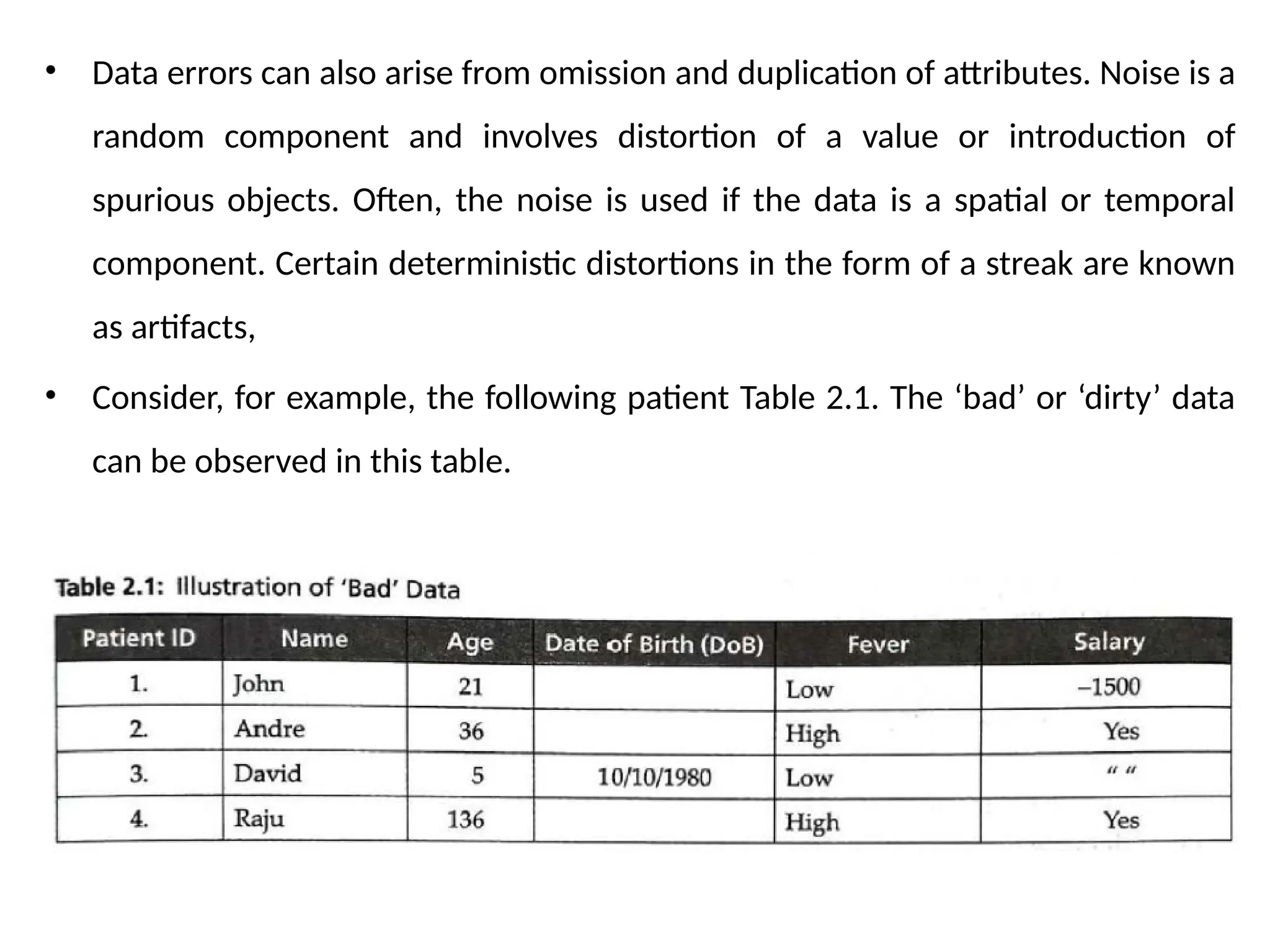
• Data errorscan also arise from omission and duplication of attributes. Noise is a
random component and involves distortion of a value or introduction of
spurious objects. Often, the noise is used if the data is a spatial or temporal
component. Certain deterministic distortions in the form of a streak are known
as artifacts,
• Consider, for example, the following patient Table 2.1. The ‘bad’ or ‘dirty’ data
can be observed in this table.
62.
• It canbe observed that data like Salary =’ ’ is incomplete data. The DoB of
patients, John, Andre, and Raju, is the missing data. The age of David is
recorded as ‘5’ but his DoB indicates it is 10/10/1980. This is called inconsistent
data.
• Inconsistent data occurs due to problems in conversions, inconsistent formats,
and difference in units. Salary for John is —1500. It cannot be less than ‘0’. It is
an instance of noisy data. Outliers are data that exhibit the characteristics that
are different from other data and have very unusual values. The age of Raju
cannot be 136. It might be a typographical error. It is often required to
distinguish between noise and outlier data.
63.
• Outliers maybe legitimate data and sometimes are of interest to the data mining
algorithms. These errors often come during data collection stage. These must be
removed so that machine learning algorithms yield better results as the quality of
results is determined by the quality of input data. This removal process is called
data cleaning.
Missing Data Analysis
• The primary data cleaning process is missing data analysis. Data cleaning routines
attempt to fill up the missing values, smoothen the noise while identifying the
outliers and correct the inconsistencies of the data. This enables data mining to
avoid overfitting of the models.
• The procedures that are given below can solve the problem of missing data:
• 1, Ignore the tuple - A tuple with missing data, especially the class label, is ignored.
This method is not effective when the percentage of the missing values increases.
64.
• 2. Fillingthe values manually — Here, the domain expert can analyse the data
tables and carry out the analysis and fill in the values manually. But, this is time
consuming and may not be feasible for larger sets.
• 3. A global constant can be used to fill in the missing attributes. The missing
values may be ‘Unknown’ or be ‘Infinity’. But, some data mining results may give
spurious results by analyzing these labels.
• 4, The attribute value may be filled by the attribute value. Say, the average
income can replace a missing value.
• 5. Use the attribute mean for all samples belonging to the same class. Here, the
average value replaces the missing values of all tuples that fall in this group.
• 6. Use the most possible value to fill in the missing value. The most probable
value can be obtained from other methods like classification and decision tree
prediction.
65.
Removal of Noisyor Outlier Data
• Noise is a random error or variance in a measured value. It can be removed by
using binning, which is a method where the given data values are sorted and
distributed into equal frequency bins.
• The bins are also called as buckets. The binning method then uses the neighbor
values to smooth the noisy data.
• Some of the techniques commonly used are ‘smoothing by means’ where the
mean of the bin removes the values of the bins, ‘smoothing by bin medians’
where the bin median replaces the bin values, and ‘smoothing by bin
boundaries’ where the bin value is replaced by the closest bin boundary.
• The maximum and minimum values are called bin boundaries. Binning methods
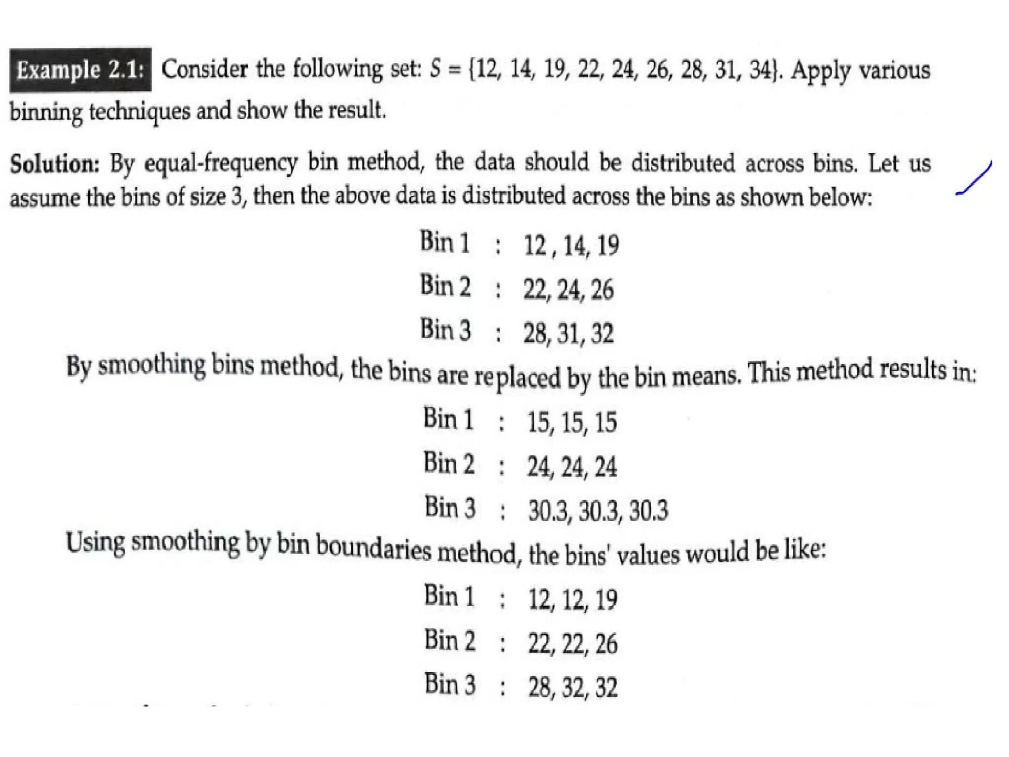
may be used as a discretization technique. Example 2.1 illustrates this principle.
67.
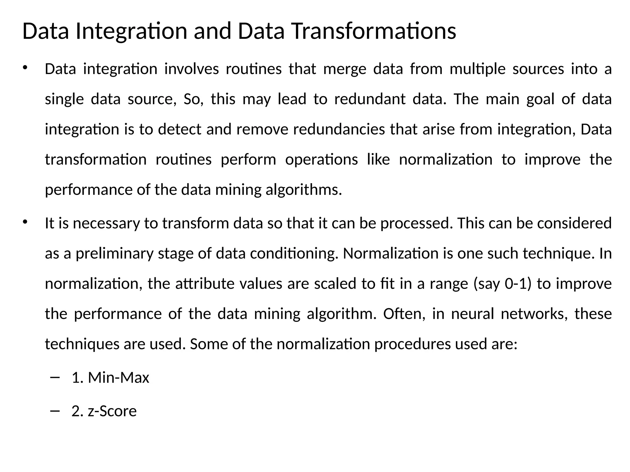
Data Integration andData Transformations
• Data integration involves routines that merge data from multiple sources into a
single data source, So, this may lead to redundant data. The main goal of data
integration is to detect and remove redundancies that arise from integration, Data
transformation routines perform operations like normalization to improve the
performance of the data mining algorithms.
• It is necessary to transform data so that it can be processed. This can be considered
as a preliminary stage of data conditioning. Normalization is one such technique. In
normalization, the attribute values are scaled to fit in a range (say 0-1) to improve
the performance of the data mining algorithm. Often, in neural networks, these
techniques are used. Some of the normalization procedures used are:
– 1. Min-Max
– 2. z-Score
68.
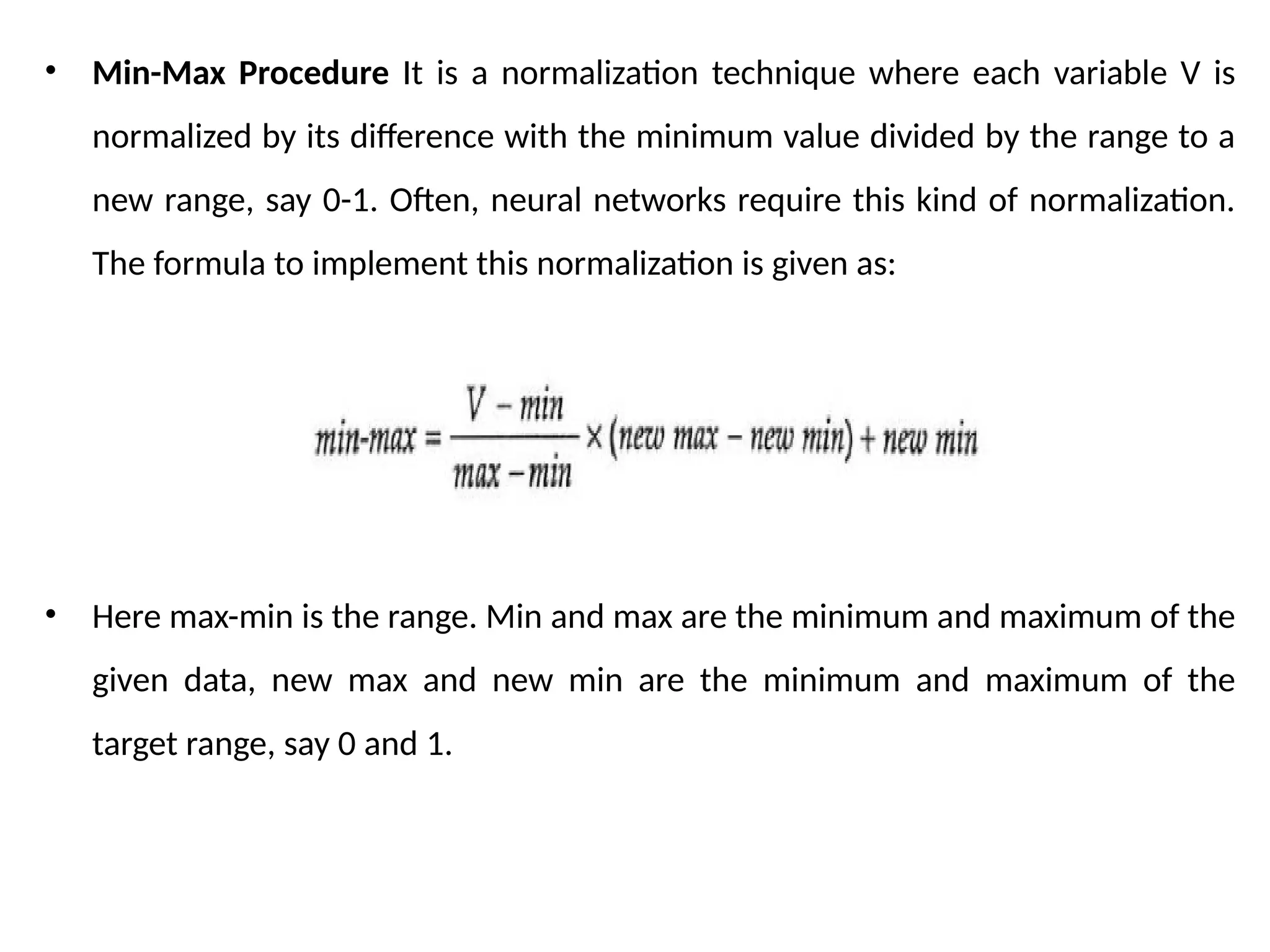
• Min-Max ProcedureIt is a normalization technique where each variable V is
normalized by its difference with the minimum value divided by the range to a
new range, say 0-1. Often, neural networks require this kind of normalization.
The formula to implement this normalization is given as:
• Here max-min is the range. Min and max are the minimum and maximum of the
given data, new max and new min are the minimum and maximum of the
target range, say 0 and 1.
70.
• So, itcan be observed that the marks (88, 90, 92, 94} are mapped to the new
range {0, 0.33, 0.66, 1). Thus, the Min-Max normalization range is between 0
and 1.
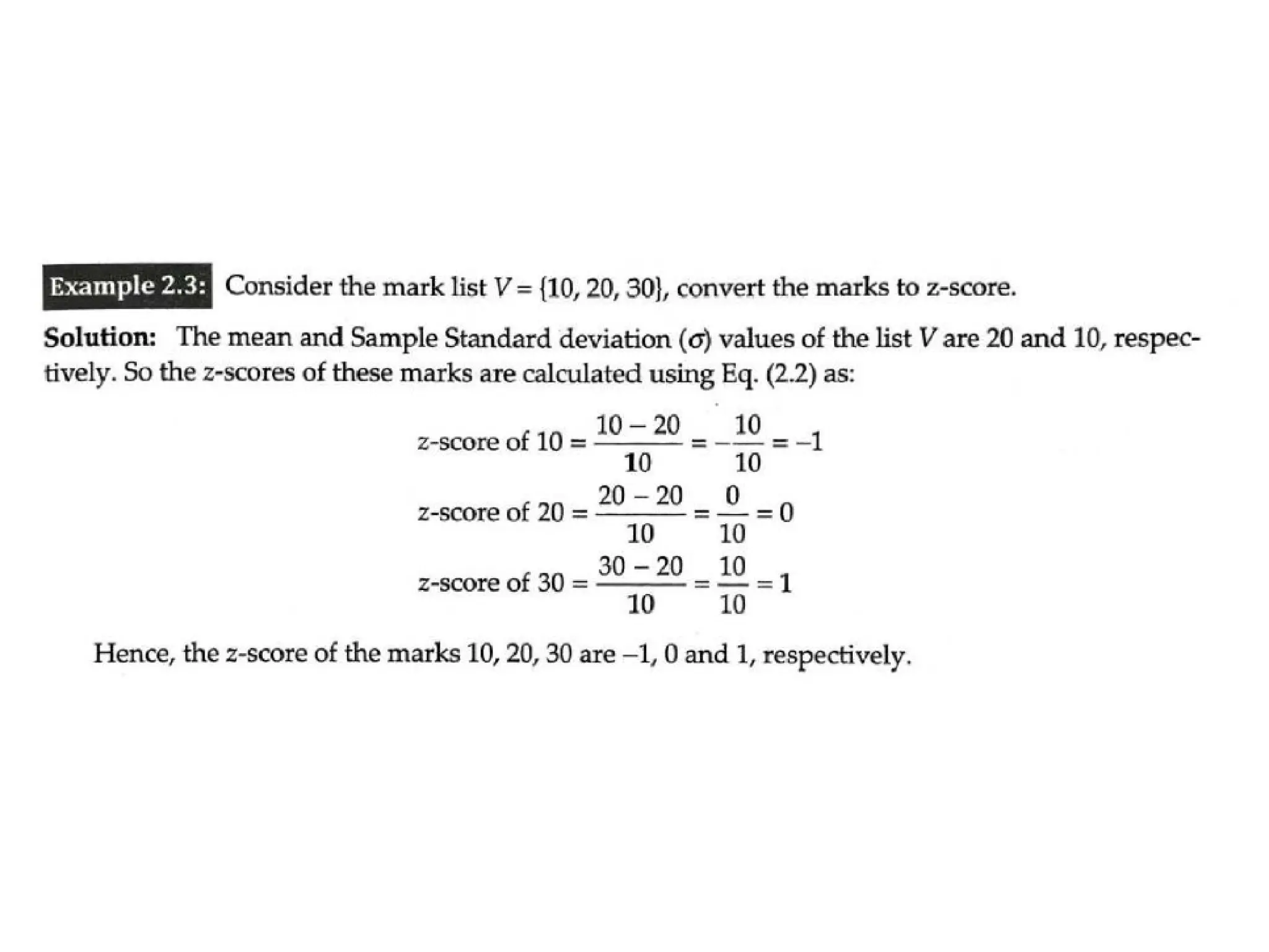
• z-Score Normalization This procedure works by taking the difference between
the field value and mean value, and by scaling this difference by standard
deviation of the attribute.
• Here, a is the standard deviation of the list V and N is the mean of the list V.
72.
Data Reduction Datareduction reduces data size but produces the same results.
There are different ways in which data reduction can be carried out such as data
aggregation, feature selection, and dimensionality
reduction.
73.
DESCRIPTIVE STATISTICS
• Descriptivestatistics is a branch of statistics that does dataset summarization. It
is used to summarize and describe data. Descriptive statistics are just
descriptive and do not go beyond that, In other words, descriptive statistics do
not bother too much about machine learning algorithms and its functioning.
• Data visualization is a branch of study that is useful for investigating the given
data. Mainly, the plots are useful to explain and present data to customers.
• Descriptive analytics and data visualization techniques help to understand the
nature of the data, which further helps to determine the kinds of machine
learning or data mining tasks that can be applied to the data. This step is often
known as Exploratory Data Analysis (EDA).
• The focus of EDA is to understand the given data and to prepare it for machine
learning algorithms. EDA includes descriptive statistics and data visualization.
74.
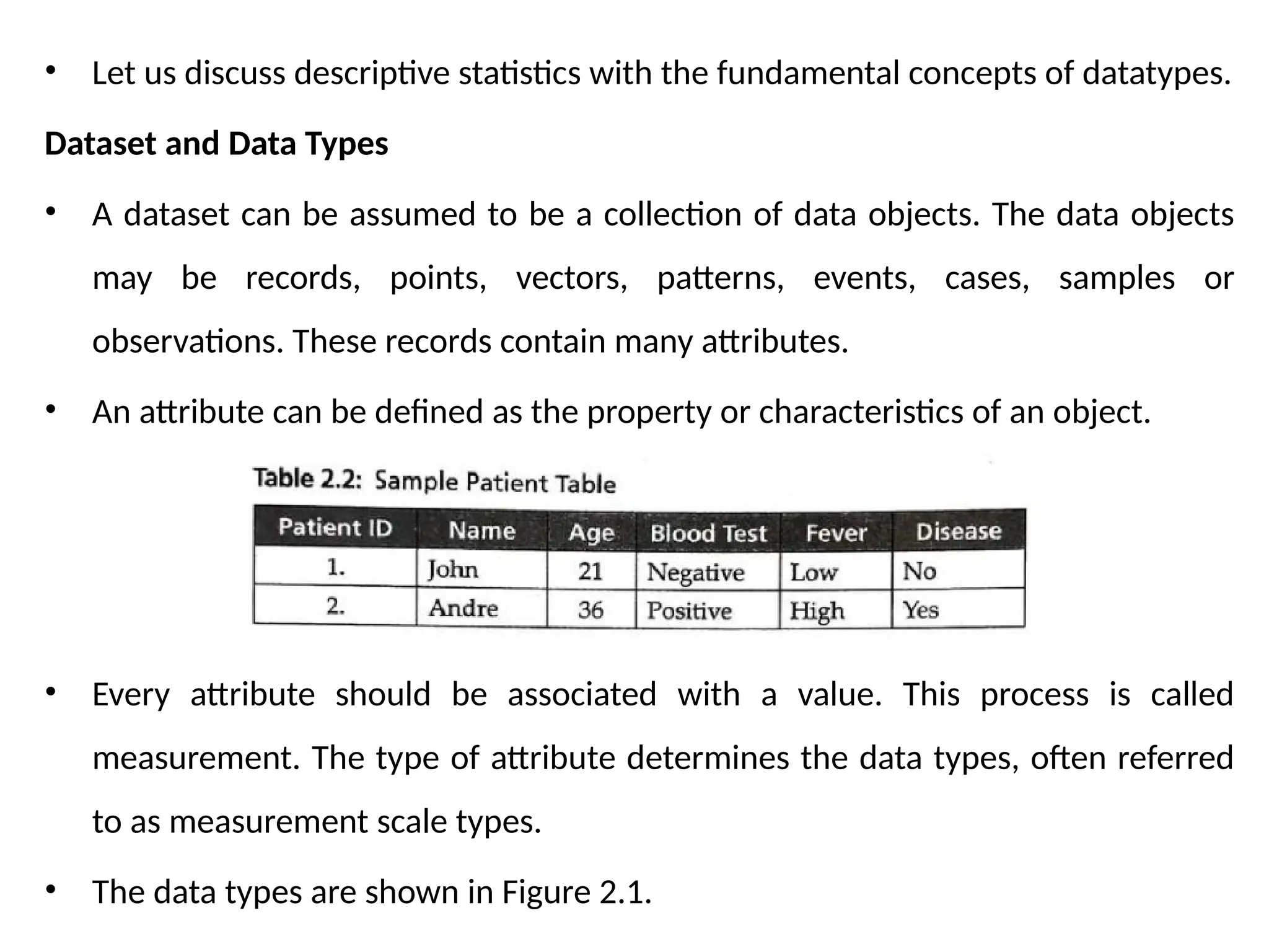
• Let usdiscuss descriptive statistics with the fundamental concepts of datatypes.
Dataset and Data Types
• A dataset can be assumed to be a collection of data objects. The data objects
may be records, points, vectors, patterns, events, cases, samples or
observations. These records contain many attributes.
• An attribute can be defined as the property or characteristics of an object.
• Every attribute should be associated with a value. This process is called
measurement. The type of attribute determines the data types, often referred
to as measurement scale types.
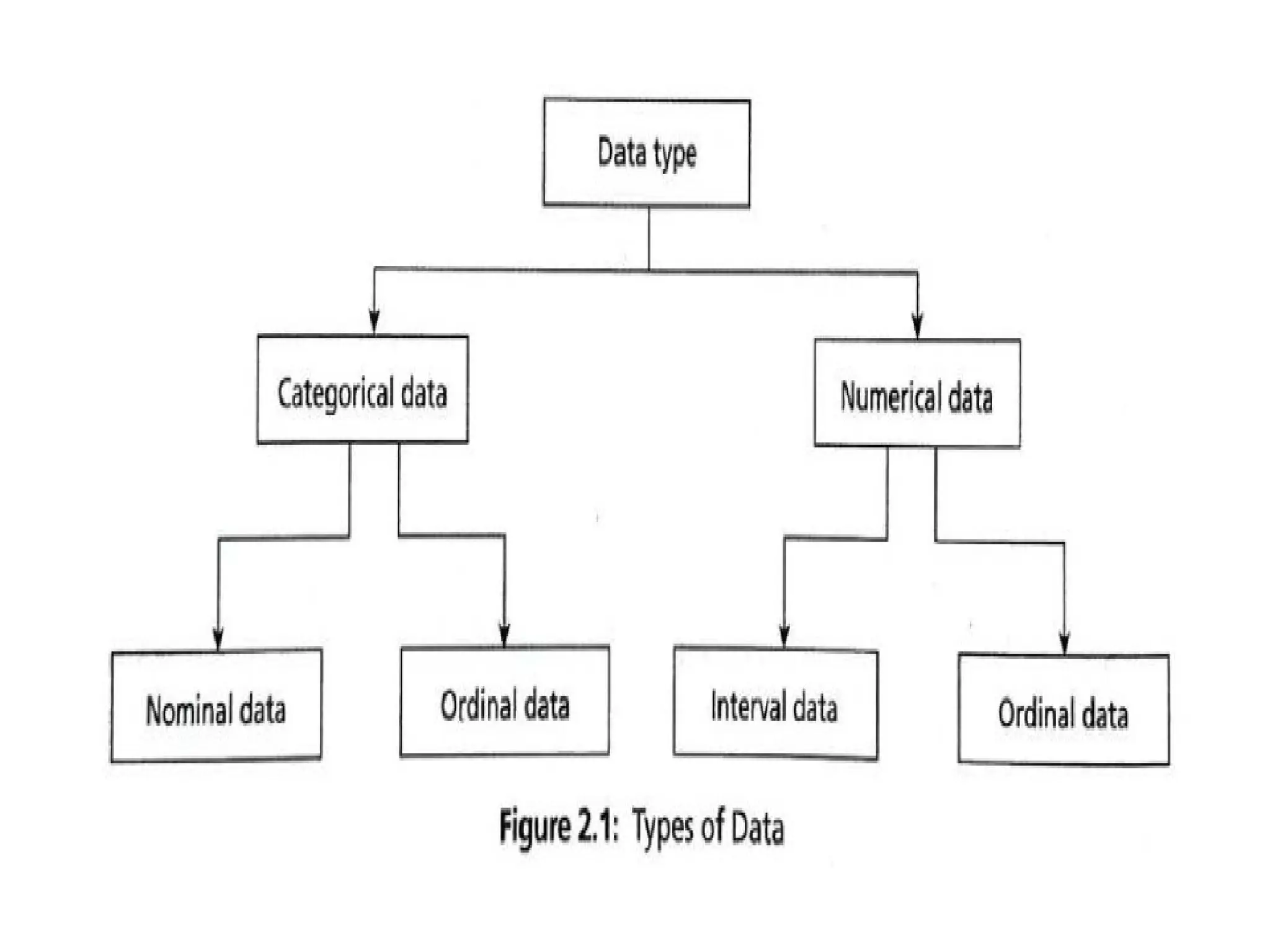
• The data types are shown in Figure 2.1.
76.
Broadly, data canbe classified into two types:
• 1. Categorical or qualitative data
• 2. Numerical or quantitative data
• Categorical or Qualitative Dare nominal type and ordinal type.ata The categorical
data can be divided into two types. They
• Nominal Data - In Table 2.2, patient ID is nominal data. Nominal data are symbols
and cannot be processed like a number. For example, the average of a patient ID
does not make any statistical sense. Nominal data type provides only information but
has no ordering among data. Only operations like (=, #) are meaningful for these
data. For example, the patient ID can be checked for equality and nothing else.
• Ordinal Data ~ It provides enough information and has natural order. For example,
Fever = {Low, Medium, High} is an ordinal data. Certainly, low is less than medium
and medium is less than high, irrespective of the value. Any transformation can be
applied to these data to get a new value.
77.
• Numeric orQualitative Data It can be divided into two categories. They are
interval type and ratio type.
• Interval Data - Interval data is a numeric data for which the differences between
values are meaningful. For example, there is a difference between 30 degree
and 40 degree. Only the permissible operations are + and -.
• Ratio Data — For ratio data, both differences and ratio are meaningful. The
difference between the ratio and interval data is the position of zero in the
scale. For example, take the Centigrade-Fahrenheit conversion. The zeroes of
both scales do not match.
• Hence, these are interval data.
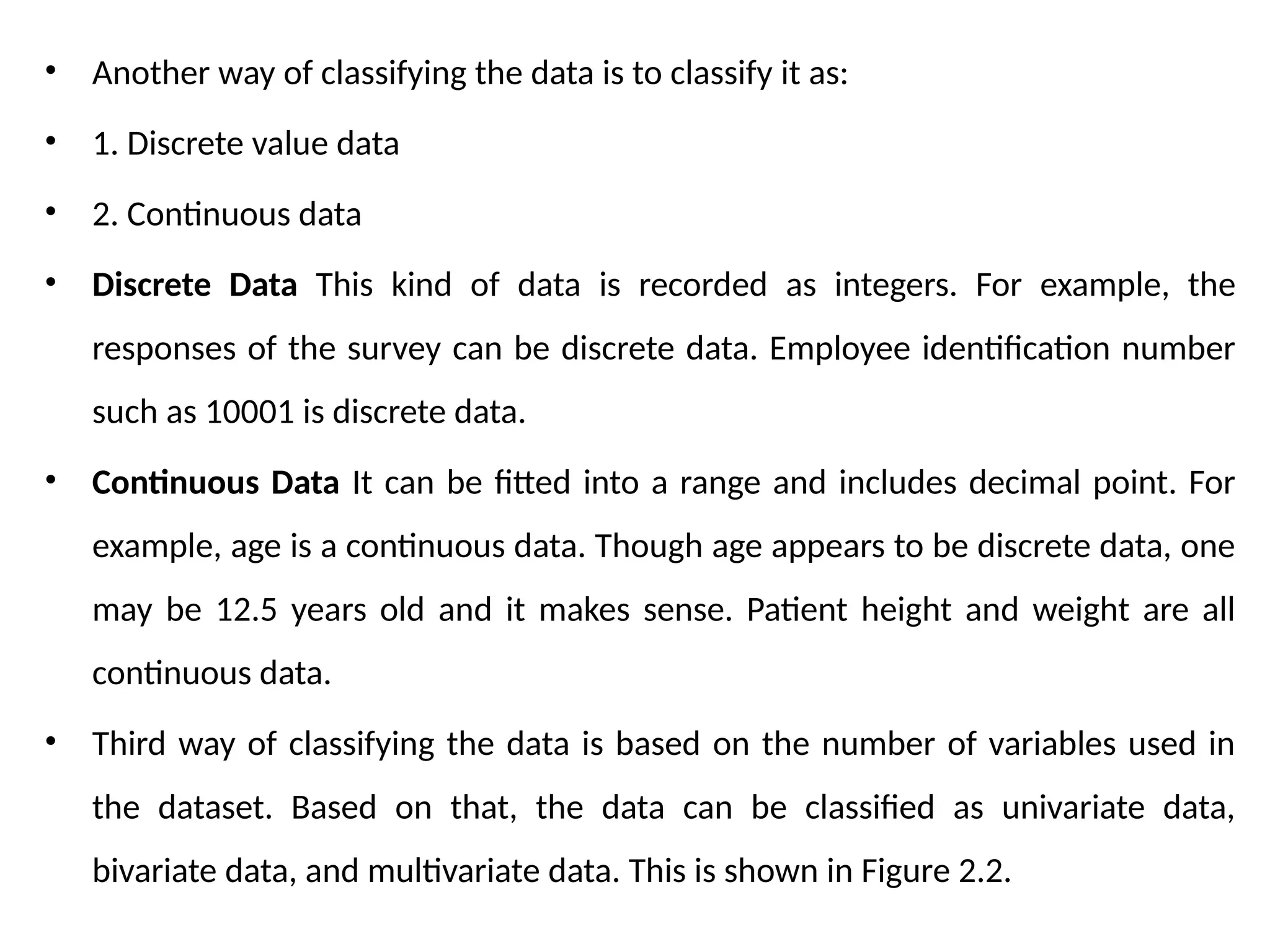
Another way of classifying the data is to classify it as:
• 1. Discrete value data
• 2. Continuous data
78.
• Another wayof classifying the data is to classify it as:
• 1. Discrete value data
• 2. Continuous data
• Discrete Data This kind of data is recorded as integers. For example, the
responses of the survey can be discrete data. Employee identification number
such as 10001 is discrete data.
• Continuous Data It can be fitted into a range and includes decimal point. For
example, age is a continuous data. Though age appears to be discrete data, one
may be 12.5 years old and it makes sense. Patient height and weight are all
continuous data.
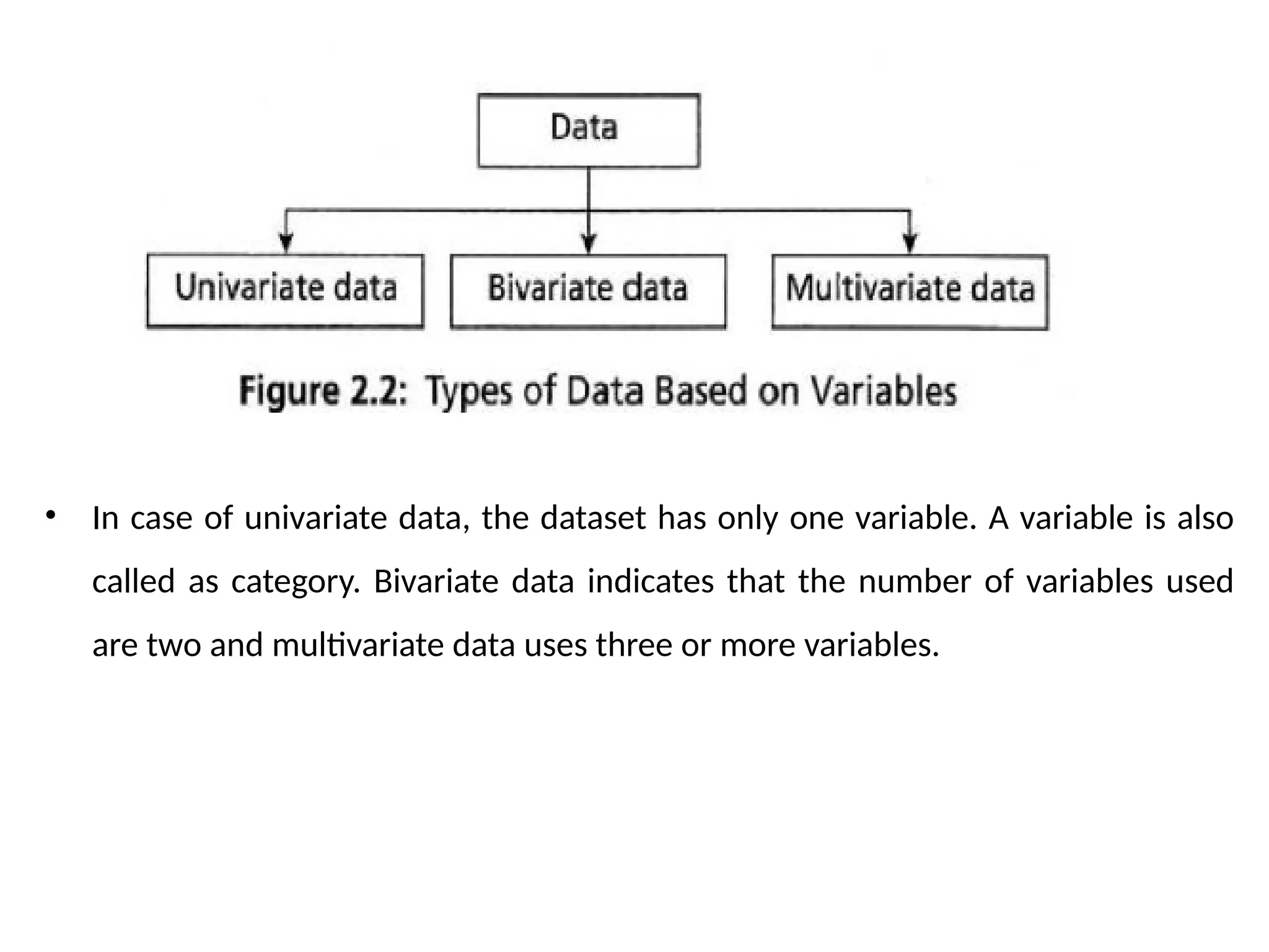
• Third way of classifying the data is based on the number of variables used in
the dataset. Based on that, the data can be classified as univariate data,
bivariate data, and multivariate data. This is shown in Figure 2.2.
79.
• In caseof univariate data, the dataset has only one variable. A variable is also
called as category. Bivariate data indicates that the number of variables used
are two and multivariate data uses three or more variables.
80.
UNIVARIATE DATA ANALYSISAND VISUALIZATION
• Univariate analysis is the simplest form of statistical analysis. As the name indicates, the
dataset has only one variable. A variable can be called asa category. Univariate does not
deal with cause or relationships. The aim of univariate analysis is to describe data and
find patterns.
• Univariate data description involves finding the frequency distributions, central tendency
measures, dispersion or variation, and shape of the data.
• Data Visualization
• To understand data, graph visualization is must. Data visualization helps to understand
data, It helps to present information and data to customers.
• Some of the graphs that are used in univariate data analysis are bar charts, histograms,
frequency polygons and pie charts.
• The advantages of the graphs are presentation of data, summarization of data, description
of data, exploration of data, and to make comparisons of data. Let us consider some forms
of graphsnow:
81.
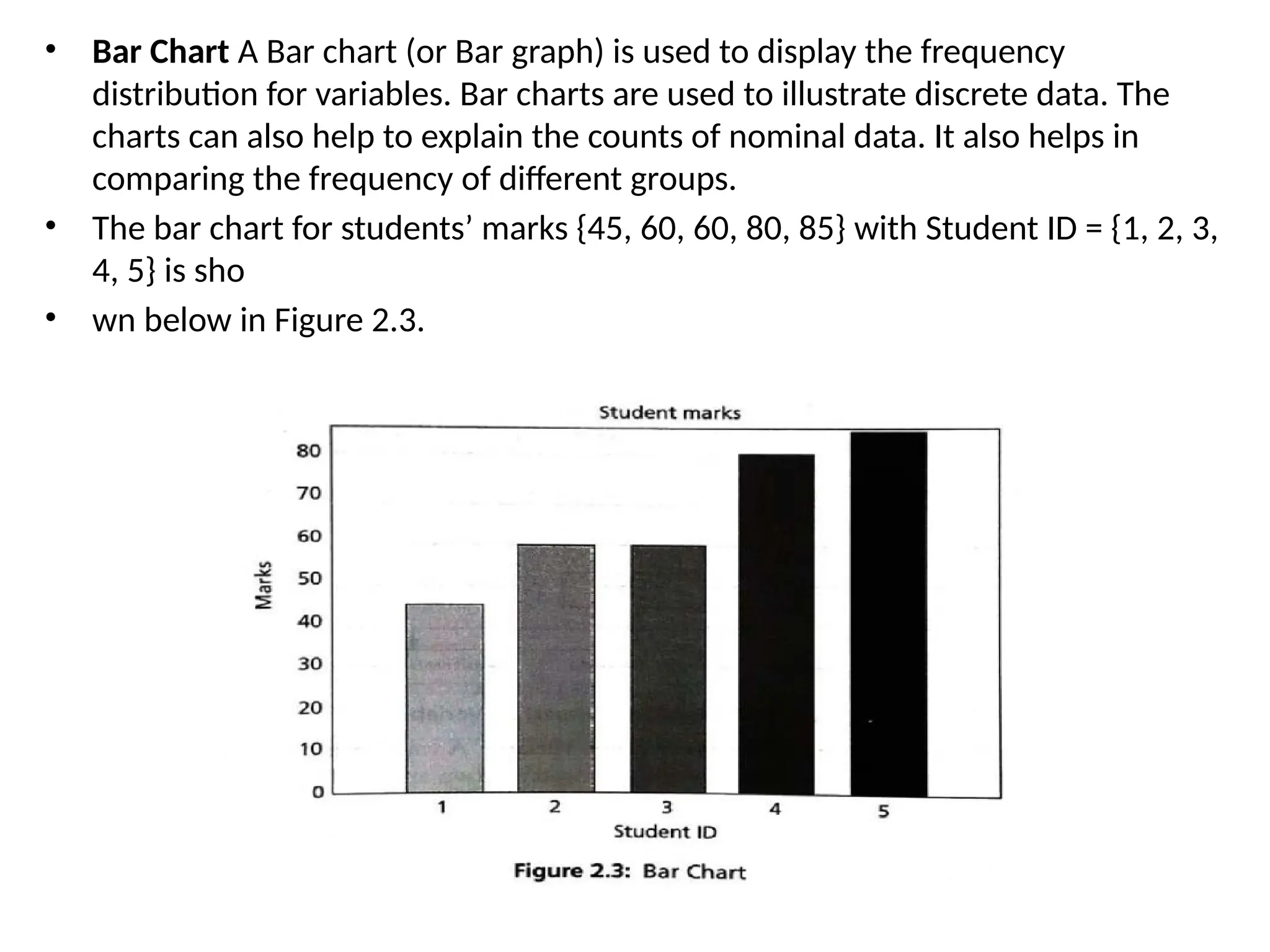
• Bar ChartA Bar chart (or Bar graph) is used to display the frequency
distribution for variables. Bar charts are used to illustrate discrete data. The
charts can also help to explain the counts of nominal data. It also helps in
comparing the frequency of different groups.
• The bar chart for students’ marks {45, 60, 60, 80, 85} with Student ID = {1, 2, 3,
4, 5} is sho
• wn below in Figure 2.3.
82.
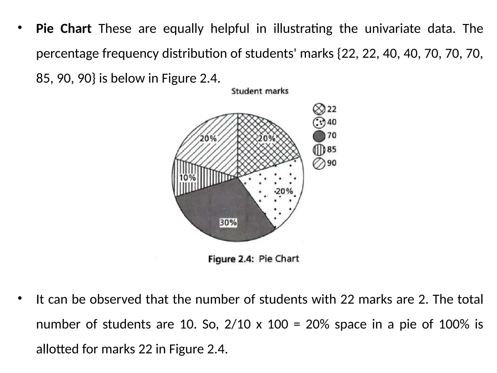
• Pie ChartThese are equally helpful in illustrating the univariate data. The
percentage frequency distribution of students' marks {22, 22, 40, 40, 70, 70, 70,
85, 90, 90} is below in Figure 2.4.
• It can be observed that the number of students with 22 marks are 2. The total
number of students are 10. So, 2/10 x 100 = 20% space in a pie of 100% is
allotted for marks 22 in Figure 2.4.
83.
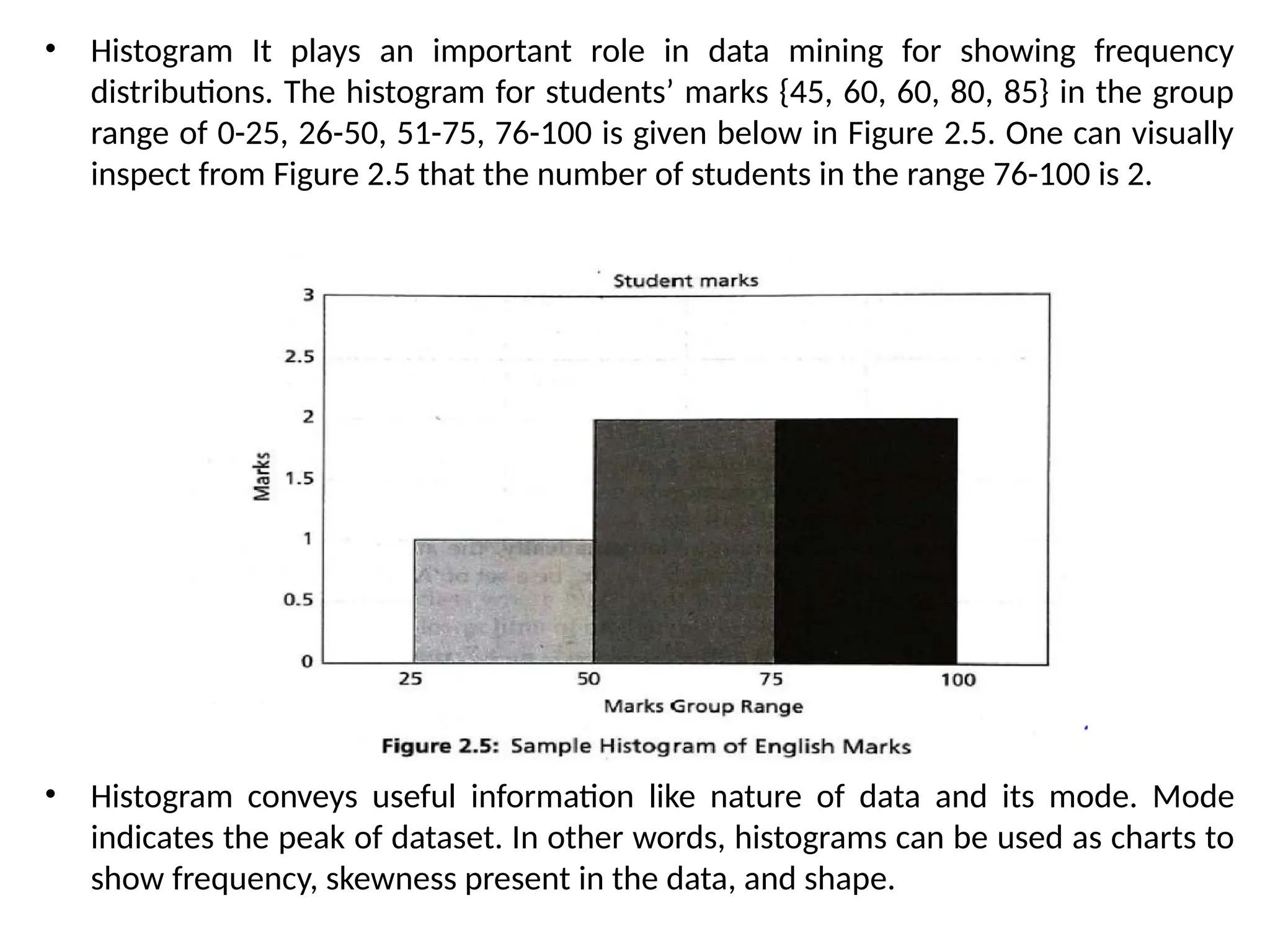
• Histogram Itplays an important role in data mining for showing frequency
distributions. The histogram for students’ marks {45, 60, 60, 80, 85} in the group
range of 0-25, 26-50, 51-75, 76-100 is given below in Figure 2.5. One can visually
inspect from Figure 2.5 that the number of students in the range 76-100 is 2.
• Histogram conveys useful information like nature of data and its mode. Mode
indicates the peak of dataset. In other words, histograms can be used as charts to
show frequency, skewness present in the data, and shape.
84.
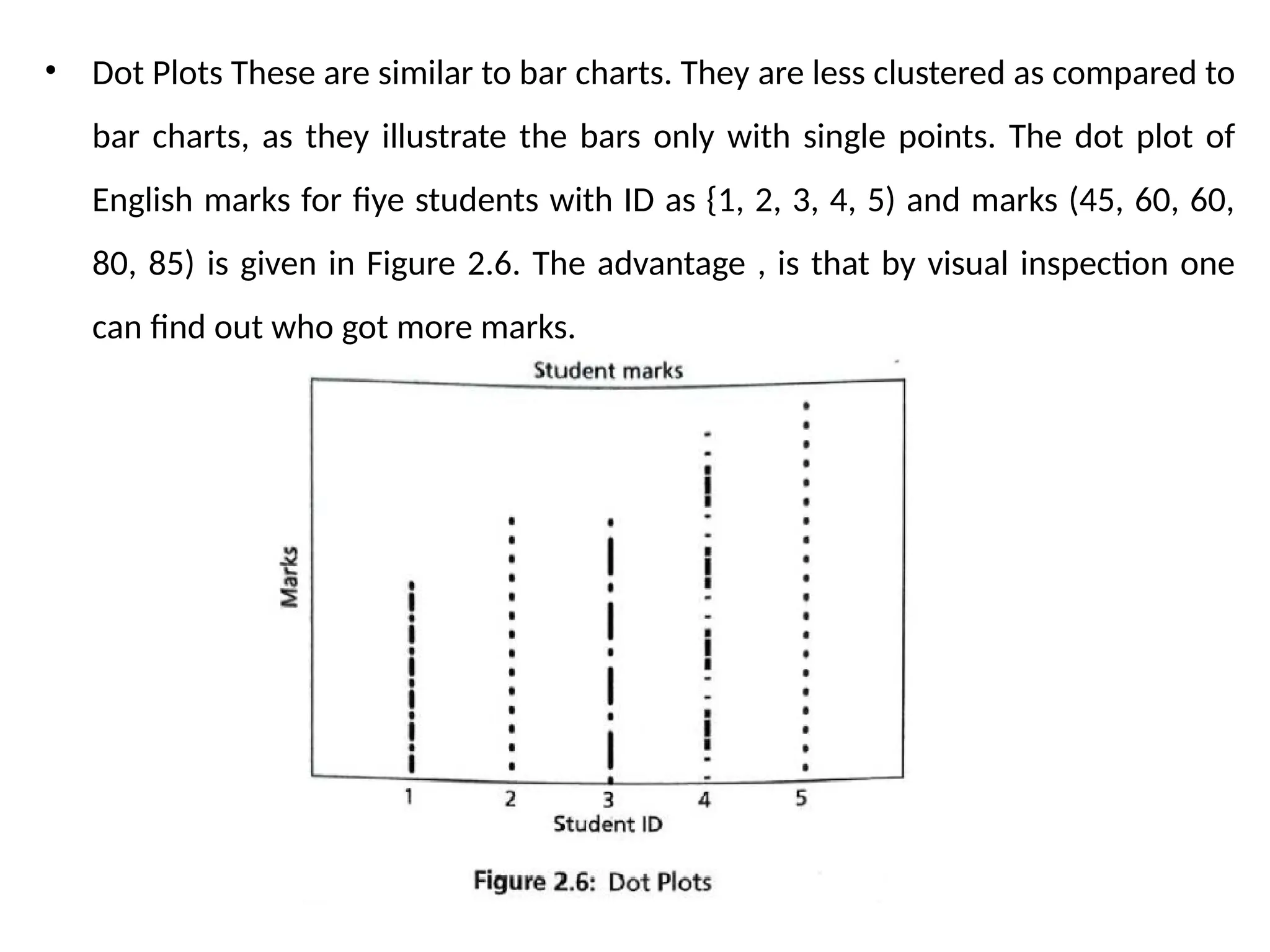
• Dot PlotsThese are similar to bar charts. They are less clustered as compared to
bar charts, as they illustrate the bars only with single points. The dot plot of
English marks for fiye students with ID as {1, 2, 3, 4, 5) and marks (45, 60, 60,
80, 85) is given in Figure 2.6. The advantage , is that by visual inspection one
can find out who got more marks.
85.
Central Tendency
• Onecannot remember all the data. Therefore, a condensation or summary of the data is
necessary, This makes the data analysis easy and simple. One such summary is called
central tendency. Thus, central tendency can explain the characteristics of data and that
further helps in comparison.
• Mass data have tendency to concentrate at certain values, normally in the central
location. It is called measure of central tendency (or averages). This represents the first
order of measures. Popular measures are mean, median and mode.
• 1. Mean — Arithmetic average (or mean) is a measure of central tendency that
represents the ‘center’ of the dataset. This is the commonest measure used in our daily
conversation such as average income or average traffic. It can be found by adding all the
data and dividing the sum by the number of observations.
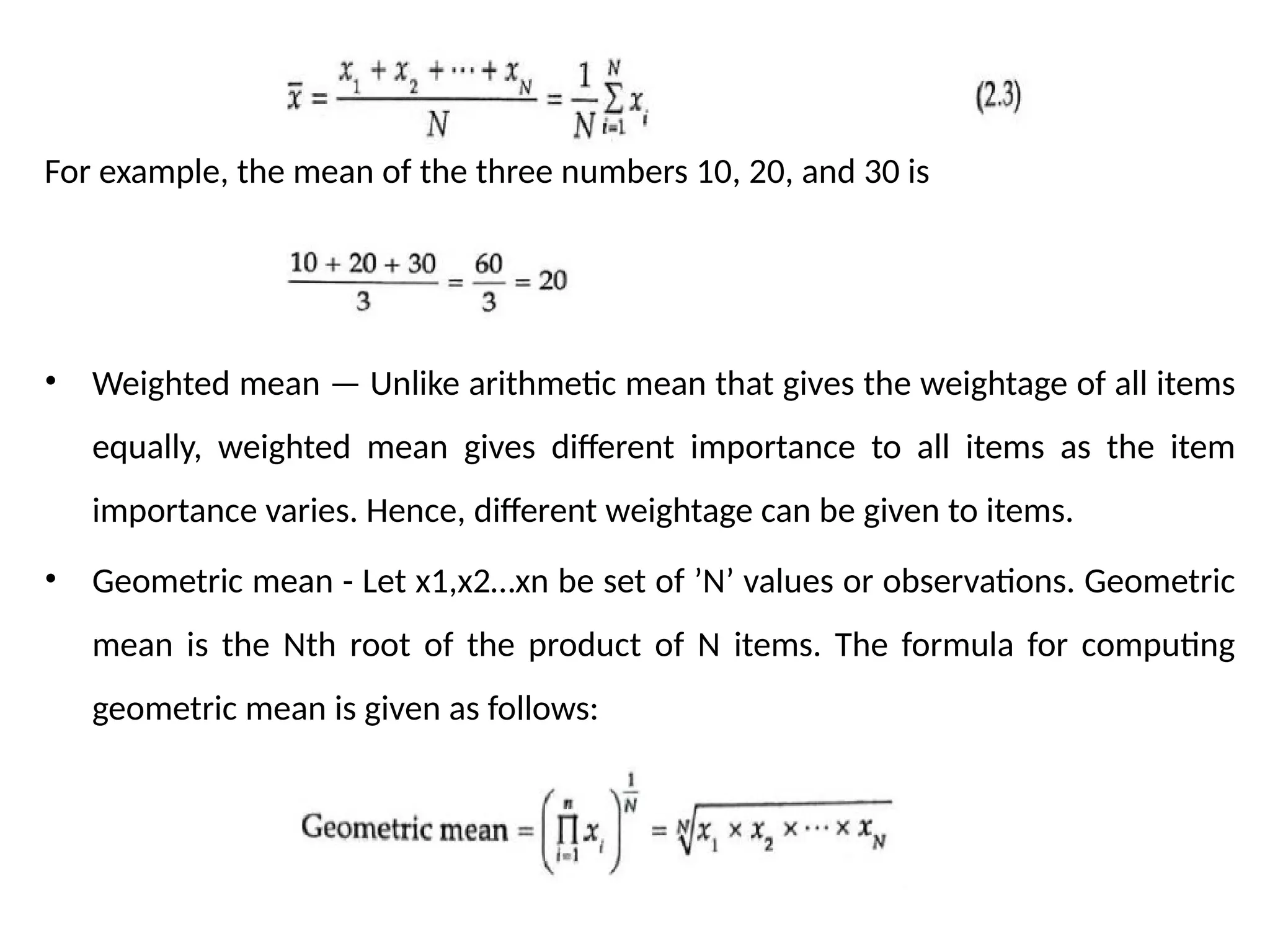
• Mathematically, the average of all the values in the sample (population) is denoted as x.
Let x1,x2…xn be a set of ‘N’ values or observations, then the arithmetic mean is given as:
86.
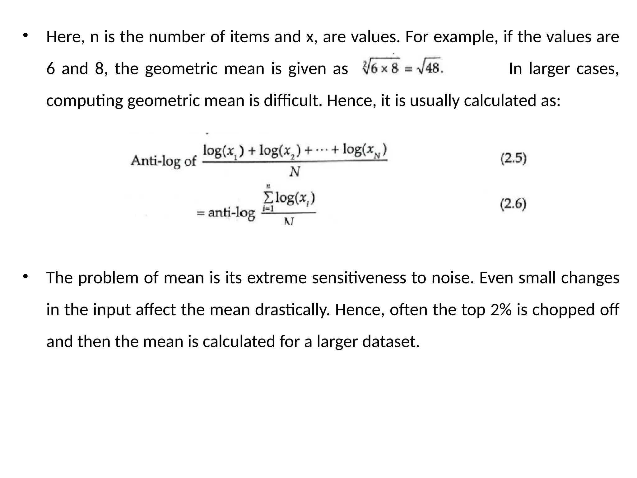
For example, themean of the three numbers 10, 20, and 30 is
• Weighted mean — Unlike arithmetic mean that gives the weightage of all items
equally, weighted mean gives different importance to all items as the item
importance varies. Hence, different weightage can be given to items.
• Geometric mean - Let x1,x2…xn be set of ’N’ values or observations. Geometric
mean is the Nth root of the product of N items. The formula for computing
geometric mean is given as follows:
87.
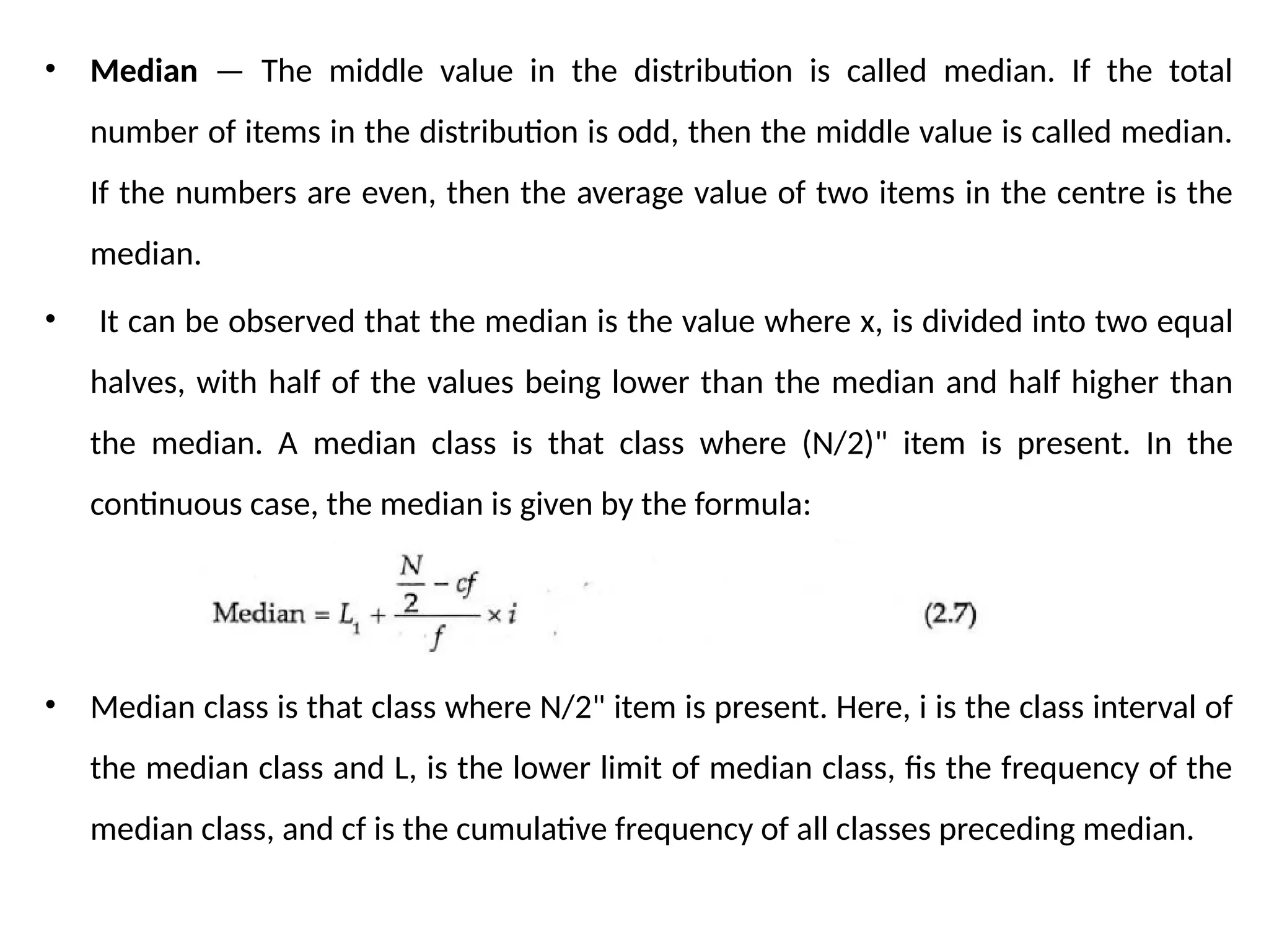
• Here, nis the number of items and x, are values. For example, if the values are
6 and 8, the geometric mean is given as . In larger cases,
computing geometric mean is difficult. Hence, it is usually calculated as:
• The problem of mean is its extreme sensitiveness to noise. Even small changes
in the input affect the mean drastically. Hence, often the top 2% is chopped off
and then the mean is calculated for a larger dataset.
88.
• Median —The middle value in the distribution is called median. If the total
number of items in the distribution is odd, then the middle value is called median.
If the numbers are even, then the average value of two items in the centre is the
median.
• It can be observed that the median is the value where x, is divided into two equal
halves, with half of the values being lower than the median and half higher than
the median. A median class is that class where (N/2)" item is present. In the
continuous case, the median is given by the formula:
• Median class is that class where N/2" item is present. Here, i is the class interval of
the median class and L, is the lower limit of median class, fis the frequency of the
median class, and cf is the cumulative frequency of all classes preceding median.
89.
• Mode -Mode is the value that occurs more frequently in the dataset. In other words, the
value that has the highest frequency is called mode. Mode is only for discrete data and is
not applicable for continuous data as there are no repeated values in continuous data.
Dispersion
• The spreadout of a set of data around the central tendency (mean, median or mode) is
called dispersion. Dispersion is represented by various ways such as range, variance,
standard deviation, and standard error. These are second order measures, The most
common measures of the dispersion data are listed below:
• Range Range is the difference between the maximum and minimum of values of the
given list of data.
• Standard Deviation The mean does not convey much more than a middle point. For
example, the following datasets {10, 20, 30} and {10, 50, 0} both have a mean of 20. The
difference between these two sets is the spread of data. Standard deviation is the
average distance from the mean of the dataset to each point.
90.
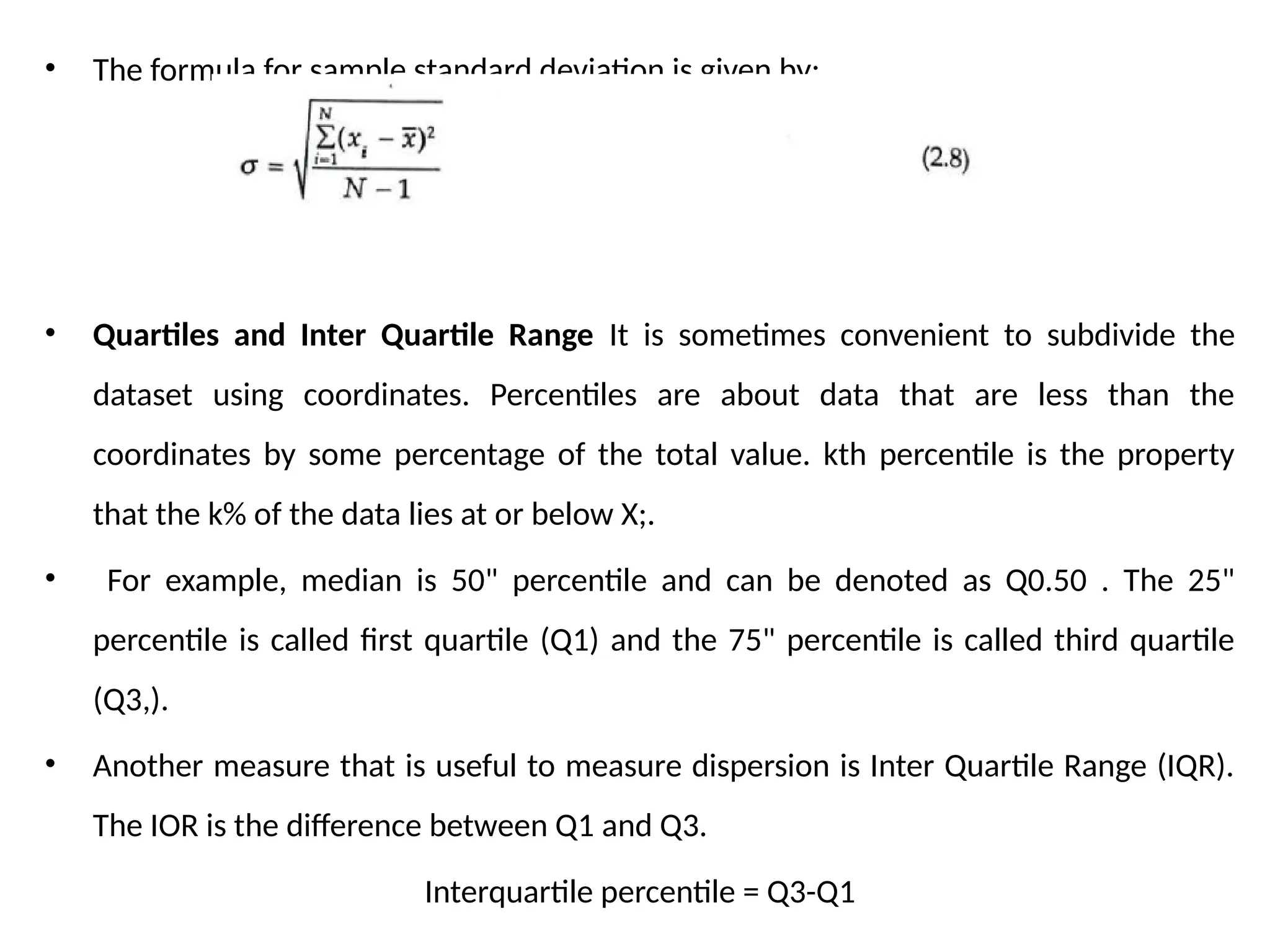
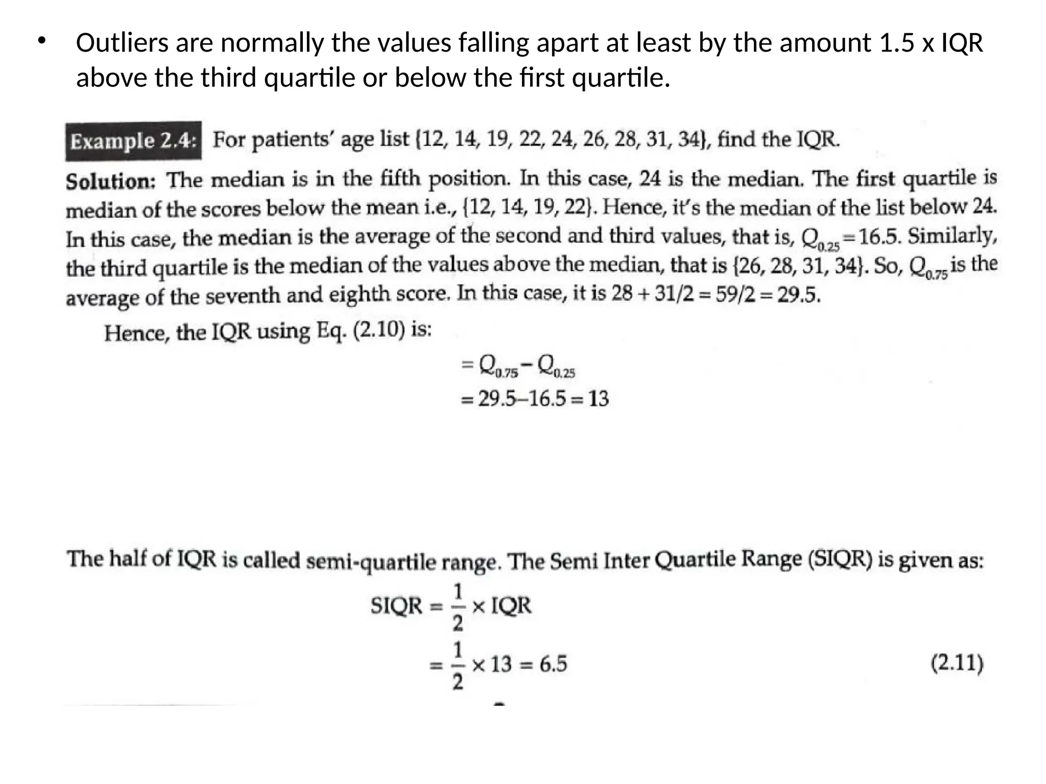
• The formulafor sample standard deviation is given by:
• Quartiles and Inter Quartile Range It is sometimes convenient to subdivide the
dataset using coordinates. Percentiles are about data that are less than the
coordinates by some percentage of the total value. kth percentile is the property
that the k% of the data lies at or below X;.
• For example, median is 50" percentile and can be denoted as Q0.50 . The 25"
percentile is called first quartile (Q1) and the 75" percentile is called third quartile
(Q3,).
• Another measure that is useful to measure dispersion is Inter Quartile Range (IQR).
The IOR is the difference between Q1 and Q3.
Interquartile percentile = Q3-Q1
91.
• Outliers arenormally the values falling apart at least by the amount 1.5 x IQR
above the third quartile or below the first quartile.
92.
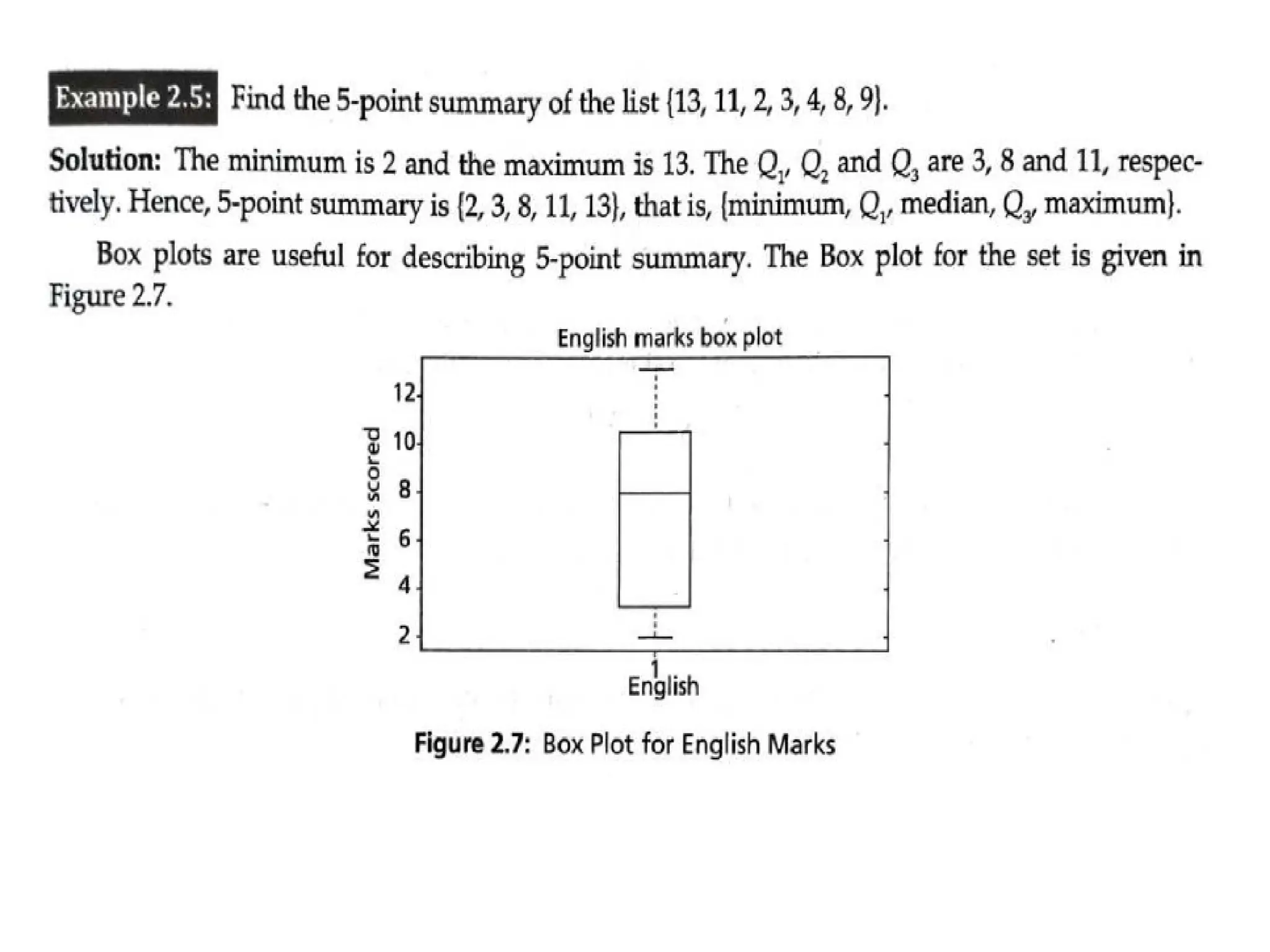
• Five-point Summaryand Box Plots The median, quartiles Q, and Q, and
minimum and maximum written in the order < Minimum, Q1, Median, Q3,
Maximum > is known as five-point summary.
• Box plots are suitable for continuous variables and a nominal variable. Box plots
can be used to illustrate data distributions and summary of data. It is the
popular way for plotting five number summaries. A Box plot is also known as a
Box and whisker plot.
• The box contains bulk of the data. These data are between first and third
quartiles. The line inside the box indicates location — mostly median of the
data. If the median is not equidistant, then the data is skewed. The whiskers
that project from the ends of the box indicate the spread of the tails and the
maximum and minimum of the data value.
94.
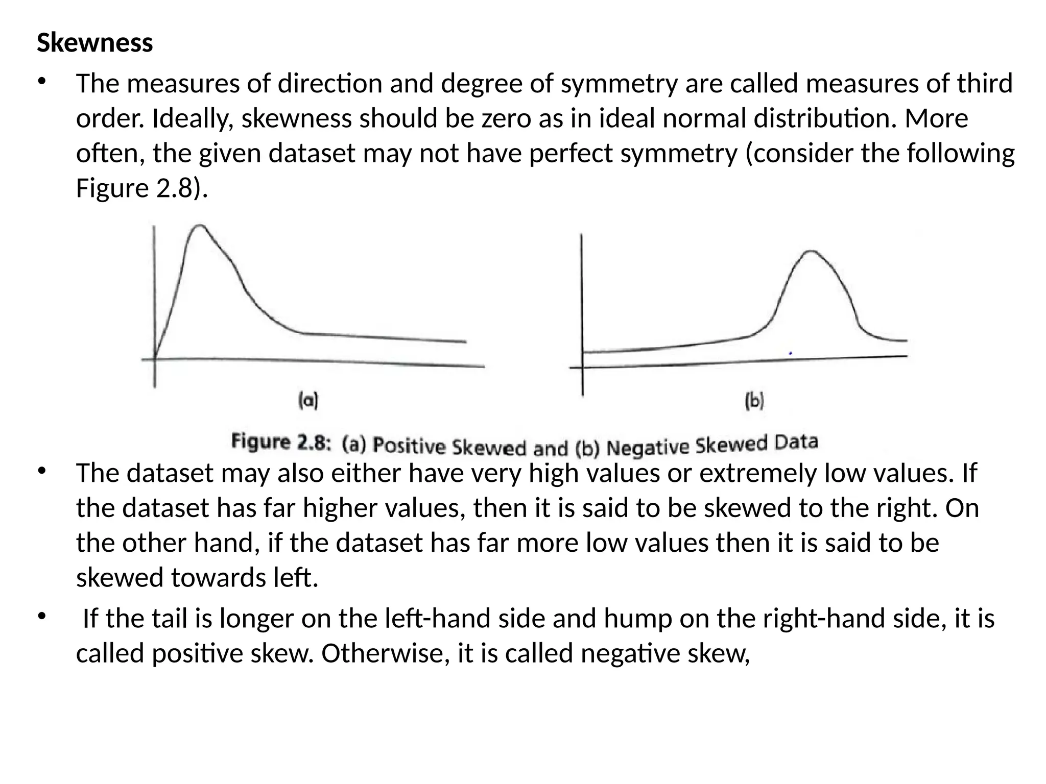
Skewness
• The measuresof direction and degree of symmetry are called measures of third
order. Ideally, skewness should be zero as in ideal normal distribution. More
often, the given dataset may not have perfect symmetry (consider the following
Figure 2.8).
• The dataset may also either have very high values or extremely low values. If
the dataset has far higher values, then it is said to be skewed to the right. On
the other hand, if the dataset has far more low values then it is said to be
skewed towards left.
• If the tail is longer on the left-hand side and hump on the right-hand side, it is
called positive skew. Otherwise, it is called negative skew,
95.
• The givendataset may have an equal distribution of data. The implication of
this is that if the data is skewed, then there is a greater chance of outliers in the
dataset. This affects the mean and median. Hence, this may affect the
performance of the data mining algorithm.
• A perfect symmetry means the skewness is zero, In the case of skew, the
median is greater than the mean.
• In positive skew, the mean is greater than the median.
• Generally, for negatively skewed distribution, the median is more than the
mean,
• The relationship between skew and the relative size of the mean and median
can be summarized by a convenient numerical skew index known as Pearson 2
skewness coefficient.
96.
• Also, thefollowing measure is more commonly used to measure skewness. Let X1,
X2..Xn. be a set of ‘N’ values or observations then the skewness can be given as:
• Here, m is the population mean and o is the population standard deviation of the
univariate data. Sometimes, for bias correction instead of N, N —1 is used.
Kurtosis
• Kurtosis also indicates the peaks of data. If the data is high peak, then it indicates
higher kurtosis and vice versa.
• Kurtosis is the measure of whether the data is heavy tailed or light tailed relative
to normal distribution. It can be observed that normal distribution has bell-shaped
curve with no long tails.
97.
• Low kurtosistends to have light tails. The implication is that there is no outlier data.
Let x1, x2,…xn be a set of ‘N’ values or observations. Then, kurtosis is measured
using the formula given below:
• It can be observed that N - 1 is used instead of N in the numerator of Eq. (2.14) for
bias correction. Here, X and o-are the mean and standard deviation of the
univariate data.
Mean Absolute Deviation (MAD)
• MAD is another dispersion measure and is robust to outliers. Normally, the outlier
point is detected by computing the deviation from median and by dividing it by
MAD. Here, the absolute deviation between the data and mean is taken. Thus, the
absolute deviation is given as:
98.
Coefficient of Variation(CV)
• Coefficient of variation is used to compare datasets with different units. CV is
the ratio of standard deviation and mean, and %CV is the percentage of
coefficient of variations.
Special Univariate Plots
• The ideal way to check the shape of the dataset is a stein and leaf plot. A stem
and leaf plot are a display that help us to know the shape and distribution of
the data. In this method, each value is split into a ‘stem’ and a ‘leaf’. The last
digit is usually the leaf and digits to the left of the leaf mostly form the stem.
• For example, marks 45 are divided into stem 4 and leaf 5 in Figure 2.9. The stem
and leaf plot for the English subject marks, say, {45, 60, 60, 80, 85} is given in
Figure 2.9.
99.
• It canbe seen from Figure 2.9 that the first column is stem and the second column
is leaf.
• For the given English marks, two students with 60 marks are shown in stem and leaf
plot as stem-6 with 2 leaves with 0.
• As discussed earlier, the ideal shape of the dataset is a bell-shaped curve. This
corresponds to normality. Most of the statistical tests are designed only for normal
distribution of data.
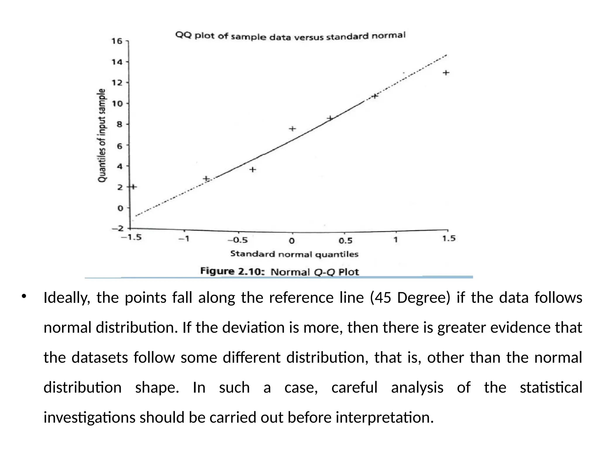
• A Q-Q plot can be used to assess the shape of the dataset. The Q-Q plot is a 2D
scatter plot of an univariate data against theoretical normal distribution data or of
two datasets — the quartiles of the first and second datasets. The normal Q-Q plot
for marks x = [13 1123 48 9] is given below in
• Figure 2.10.
100.
• Ideally, thepoints fall along the reference line (45 Degree) if the data follows
normal distribution. If the deviation is more, then there is greater evidence that
the datasets follow some different distribution, that is, other than the normal
distribution shape. In such a case, careful analysis of the statistical
investigations should be carried out before interpretation.

![• It can be seen from Figure 2.9 that the first column is stem and the second column
is leaf.
• For the given English marks, two students with 60 marks are shown in stem and leaf
plot as stem-6 with 2 leaves with 0.
• As discussed earlier, the ideal shape of the dataset is a bell-shaped curve. This
corresponds to normality. Most of the statistical tests are designed only for normal
distribution of data.
• A Q-Q plot can be used to assess the shape of the dataset. The Q-Q plot is a 2D
scatter plot of an univariate data against theoretical normal distribution data or of
two datasets — the quartiles of the first and second datasets. The normal Q-Q plot
for marks x = [13 1123 48 9] is given below in
• Figure 2.10.](https://image.slidesharecdn.com/module-1-250802063751-4b583002/75/MODULE-1-pptx-machine-learning-note-for-6th-sem-vtu-99-2048.jpg)


![Vibe Coding vs. Spec-Driven Development [Free Meetup]](https://cdn.slidesharecdn.com/ss_thumbnails/vibecodingvsspecdrivendevelopment-251209105622-43f455e7-thumbnail.jpg?width=640&height=640&fit=bounds)


