The document discusses modeling the economics of catastrophic climate change caused by structural uncertainty. It argues that uncertainty can induce "fat tails" in predictive distributions, increasing the probability of extreme negative impacts. This has strong implications for situations like climate change where catastrophe is theoretically possible. The paper aims to present a rigorous economic-statistical model of this issue and show that fat tails from structural uncertainty can potentially outweigh the effects of discounting in climate change policy analysis. It uses climate sensitivity as a hypothetical example of an uncertain scaling factor that could have significant fat tails, increasing the probability of temperature changes like 10°C or more that could cause worldwide catastrophe.

1. The Review of Economics and Statistics
VOL. XCI NUMBER 1
FEBRUARY 2009
ON MODELING AND INTERPRETING THE ECONOMICS OF
CATASTROPHIC CLIMATE CHANGE
Martin L. Weitzman*
Abstract—With climate change as prototype example, this paper analyzes
the implications of structural uncertainty for the economics of low-
probability, high-impact catastrophes. Even when updated by Bayesian
learning, uncertain structural parameters induce a critical “tail fattening”
of posterior-predictive distributions. Such fattened tails have strong im-
plications for situations, like climate change, where a catastrophe is
theoretically possible because prior knowledge cannot place sufficiently
narrow bounds on overall damages. This paper shows that the economic
consequences of fat-tailed structural uncertainty (along with unsureness
about high-temperature damages) can readily outweigh the effects of
discounting in climate-change policy analysis.
I. Introduction
WHAT is the essence of the economic problem posed
by climate change? The economic uniqueness of the
climate-change problem is not just that today’s decisions
have difficult-to-reverse impacts that will be felt very far out
into the future, thereby straining the concept of time dis-
counting and placing a heavy burden on the choice of an
interest rate. Nor does uniqueness come from the unsure
outcome of a stochastic process with known structure and
known objective-frequency probabilities. Much more unset-
tling for an application of (present discounted) expected
utility analysis are the unknowns: deep structural uncer-
tainty in the science coupled with an economic inability to
evaluate meaningfully the catastrophic losses from disas-
trous temperature changes. The climate science seems to be
saying that the probability of a disastrous collapse of plan-
etary welfare is nonnegligible, even if this tiny probability is
not objectively knowable. Motivated by the climate-change
example, this paper presents a mathematically rigorous (but
abstract) economic-statistical model of high-impact, low-
probability catastrophes. It also presents some less rigorous
numerical calculations suggesting the empirical importance
for climate-change analysis of the surprisingly strong theo-
retical result from the abstract model. The least rigorous part
of the paper concludes with some speculative (but, I think,
necessary) thoughts about what this all means for climate-
change policy.
The next section argues that, were one forced to specify
a “best guess” estimate of the extreme bad tail of the
relevant probability density function (PDF) of what might
eventually happen if only gradually ramped-up remedies are
applied, then mean global surface temperature change rel-
ative to pre-industrial-revolution levels will in two centuries
or so be greater than 10°C with a ballpark probability
estimate somewhere around 0.05 and will be greater than
20°C with a ballpark probability estimate somewhere
around 0.01. Societies and ecosystems in a world whose
average temperature has changed in the geologically instan-
taneous time of two centuries or so by 10°C–20°C (for U.S.
readers: a change of 10°C ⫽ a change of 18°F and a change
of 20°C ⫽ a change of 36°F) are located in terra incognita,
since such high temperatures have not existed for hundreds
of millions of years and such a rate of global temperature
change might be unprecedented even on a timescale of
billions of years. However measured, the planetary welfare
effect of climate changes that might accompany mean
temperature increases from 10°C up to 20°C with probabil-
ities anything remotely resembling 5% down to 1% implies
a nonnegligible probability of worldwide catastrophe. The
paper suggests that the shock value of this kind of numerical
example may not be accidental. Rather, it might stem from
a deeply rooted theoretical principle—thereby delivering a
combined theoretical-empirical punch that is particularly
potent for climate-change analysis.
In his book Catastrophe: Risk and Response,1 Richard
Posner defines the word “catastrophe” “to designate an
event that is believed to have a very low probability of
materializing but that if it does materialize will produce a
harm so great and sudden as to seem discontinuous with the
flow of events that preceded it.” Posner adds: “The low
probability of such disasters—frequently the unknown prob-
ability, as in the case of bioterrorism and abrupt global
warming—is among the things that baffle efforts at respond-
ing rationally to them.” In this paper I address what a
Received for publication October 16, 2007. Revision accepted for
publication June 23, 2008.
* Department of Economics, Harvard University.
Without blaming them for remaining deficiencies of the paper, I am
extremely grateful for the constructive comments of Frank Ackerman,
Roland Benabou, Richard Carson, Daniel Cole, Stephen DeCanio, Don
Fullerton, Olle Häggström, Robert Hahn, John Harte, Peter Huybers, Reto
Knutti, Karl Löfgren, Michael Mastrandrea, Robert Mendelsohn, Gilbert
Metcalf, William Nordhaus, Cedric Philibert, Robert Pindyck, Richard
Posner, John Reilly, Daniel Schrag, Cass Sunstein, Richard Tol, Gary
Yohe, and Richard Zeckhauser.
1 Posner (2004). See also the insightful review by Parson (2007).
Sunstein (2007) covers some similar themes more analytically and from a
somewhat different perspective.
The Review of Economics and Statistics, February 2009, 91(1): 1–19
© 2009 by the President and Fellows of Harvard College and the Massachusetts Institute of Technology

2. rational economic response in the discipline-imposing form
of (present discounted) expected utility theory might offer
by way of guidance for thinking coherently about the
economics of uncertain catastrophes with tiny but highly
unknown probabilities.
Modeling uncertain catastrophes presents some very
strong challenges to economic analysis, the full implications
of which have not yet been adequately confronted. Cost-
benefit analysis (CBA) based on expected utility (EU)
theory has been applied in practice primarily to cope with
uncertainty in the form of a known thin-tailed PDF. This
paper shows that there is a rigorous sense in which the
relevant posterior-predictive PDF of high-impact, low-
probability catastrophes has a built-in tendency to be fat
tailed. A fat-tailed PDF assigns a relatively much higher
probability to rare events in the extreme tails than does a
thin-tailed PDF.2 (Even though both limiting probabilities
are infinitesimal, the ratio of a thick-tailed probability
divided by a thin-tailed probability approaches infinity in
the limit.) Not much thought has gone into conceptualizing
or modeling what happens to EU-based CBA for fat-tailed
disasters. A CBA of a situation with known thin tails, even
including whatever elements of subjective arbitrariness it
might otherwise contain, can at least in principle make
comforting statements of the generic form: “If the PDF tails
are cut off here, then EU theory will still capture and convey
an accurate approximation of what is important.” Such
accuracy-of-approximation PDF-tail-cutoff statements, alas,
do not exist in this generic sense for what in this paper I am
calling “fat-tailed CBA.”
Fat-tailed CBA has strong implications that have been
neither recognized in the literature nor incorporated into
formal CBA modeling of disasters like climate-change ca-
tastrophes. These implications raise many disturbing yet
important questions, which will be dealt with somewhat
speculatively in the concluding sections of this paper. Par-
tially answered questions and speculative thoughts aside, I
contend it is nevertheless undeniable that, at least in prin-
ciple, fat-tailed CBA can turn conventional thin-tail-based
climate-change policy advice on its head. This paper shows
that it is quite possible, and even numerically plausible, that
the answers to the big policy question of what to do about
climate change stand or fall to a large extent on the issue of
how the high-temperature damages and tail probabilities are
conceptualized and modeled. By implication, the policy
advice coming out of conventional thin-tailed CBAs of
climate change must be treated with skepticism until this
low-probability, high-impact aspect is addressed seriously
and included empirically in a true fat-tailed CBA.
Standard approaches to modeling the economics of cli-
mate change (even those that purport to treat risk by Monte
Carlo simulations) very likely fail to account adequately for
the implications of large impacts with small probabilities.
From inductive experience alone, one cannot acquire suffi-
ciently accurate information about the probabilities of ex-
treme tail disasters to prevent the expected marginal utility
of an extra unit of consumption from becoming infinite for
any utility function with relative risk aversion everywhere
bounded above 0. To close the model in the sense of making
expected marginal utility be below ⫹⬁ (or expected utility
above ⫺⬁), the paper relies on a concept akin to the “value
of statistical life” (VSL)—except that here it represents
something more like the rate of substitution between con-
sumption and the mortality risk of a catastrophic extinction
of civilization or the natural world as we know these
concepts. With this way of closing the model (which, I will
argue, is at least better than the alternatives), subsequent
EU-based CBA then depends critically upon an exog-
enously imposed VSL-like parameter that is a generaliza-
tion of the value of a statistical human life and is presum-
ably very big. Practically, a high VSL-like parameter means
for open-ended situations with potentially unlimited down-
side exposure (like climate change) that a Monte Carlo
simulation must go very deep into the extreme-negative-
impact fat tail to merit credibility as an accurate and fair
CBA. In this sense (by making there be such utter depen-
dence upon a concept like the value of a statistical life,
which might be very big), structural or deep uncertainty is
potentially much more of a driving force than discounting or
pure risk. For situations where there do not exist prior limits
on damages (like climate change from greenhouse warm-
ing), CBA is likely to be dominated by considerations and
concepts related more to catastrophe insurance than to the
consumption smoothing consequences of long-term dis-
counting—even at empirically plausible interest rates.
II. Generalized Climate Sensitivity as a Scaling Factor
The broad thesis of this paper is that PDF tails fattened by
structural uncertainty can have a big effect on CBA. The
specific example I use to illustrate this thesis is a critical
scale parameter that multiplies or amplifies an exogenous
shock or perturbation to the system. The purpose of this
section is to motivate heuristically, and to derive some
extremely crude ballpark numerical estimates for the tail
PDF of, this kind of scaling-transfer factor in a context of
climate change. Very roughly—at a very high level of
abstraction and without trying to push an imperfect analogy
too far—the generic role of this uncertain multiplicative
amplifier or scale parameter might perhaps be illustrated by
the role of an uncertain “climate sensitivity” coefficient in
climate-change models and discussions of global warming.
2 As I use the term in this paper a PDF has a “fat” (or “thick” or “heavy”)
tail when its moment generating function (MGF) is infinite—that is, the
tail probability approaches 0 more slowly than exponentially. The standard
example of a fat-tailed PDF is the power law (aka polynomial aka Pareto)
distribution, although, for example, a log normal PDF is also fat tailed, as
is an inverted-normal or inverted-gamma. By this definition a PDF whose
MGF is finite has a “thin” tail. A normal or a gamma are examples of
thin-tailed PDFs, as is any PDF having finite supports. As shown later, the
welfare significance of fat versus thin tails comes via a tight connection
between the CRRA EU of consumption and the MGF of consumption
growth.
THE REVIEW OF ECONOMICS AND STATISTICS
2

3. Climate sensitivity is a key macro-indicator of the even-
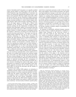
tual temperature response to greenhouse gas (GHG)
changes. Let ⌬ ln CO2 be sustained relative change in
atmospheric carbon dioxide while ⌬T is equilibrium tem-
perature response. Narrowly defined, climate sensitivity
(here denoted S1) converts ⌬ ln CO2 into ⌬T by the formula
⌬T ⬇ (S1/ln 2) ⫻ ⌬ ln CO2. As the Intergovernmental
Panel on Climate Change in its IPCC-AR4 (2007) executive
summary puts it: “The equilibrium climate sensitivity is a
measure of the climate system response to sustained radia-
tive forcing. It is not a projection but is defined as the global
average surface warming following a doubling of carbon
dioxide concentrations. It is likely to be in the range 2°C to
4.5°C with a best estimate of 3°C, and is very unlikely to be
less than 1.5°C. Values substantially higher than 4.5°C
cannot be excluded, but agreement of models with obser-
vations is not as good for those values.” Climate sensitivity
is not the same as temperature change, but for the benchmark-
serving purposes of my simplistic example I assume the
shapes of both PDFs are roughly similar after approxi-
mately 200 years because a doubling of anthropogenically
injected CO2-equivalent (CO2-e) GHGs relative to pre-
industrial-revolution levels is essentially unavoidable within
about the next 40 years and will plausibly remain well
above two times preindustrial levels for at least 100 or more
years thereafter.
In this paper I am mostly concerned with the roughly
15% of those S1 “values substantially higher than 4.5°C”
which “cannot be excluded.” A grand total of 22 peer-
reviewed studies of climate sensitivity published recently in
reputable scientific journals and encompassing a wide vari-
ety of methodologies (along with 22 imputed PDFs of S1)
lie indirectly behind the above-quoted IPCC-AR4 (2007)
summary statement. These 22 recent scientific studies cited
by IPCC-AR4 are compiled in table 9.3 and box 10.2. It
might be argued that these 22 studies are of uneven reli-
ability and their complicatedly related PDFs cannot easily
be combined, but for the simplistic purposes of this illus-
trative example I do not perform any kind of formal Bayes-
ian model-averaging or meta-analysis (or even engage in
informal cherry picking). Instead I just naively assume that
all 22 studies have equal credibility and for my purposes
here their PDFs can be simplistically aggregated. The upper
5% probability level averaged over all 22 climate-sensitivity
studies cited in IPCC-AR4 (2007) is 7°C while the median
is 6.4°C,3 which I take as signifying approximately that
P[S1 ⬎ 7⬚C] ⬇ 5%. Glancing at table 9.3 and box 10.2 of
IPCC-AR4, it is apparent that the upper tails of these 22
PDFs tend to be sufficiently long and fat that one is allowed
from a simplistically aggregated PDF of these 22 studies the
rough approximation P[S1 ⬎ 10⬚C] ⬇ 1%. The actual
empirical reason why these upper tails are long and fat
dovetails beautifully with the theory of this paper: inductive
knowledge is always useful, of course, but simultaneously it
is limited in what it can tell us about extreme events outside
the range of experience—in which case one is forced back
onto depending more than one might wish upon the prior
PDF, which of necessity is largely subjective and relatively
diffuse. As a recent Science commentary put it: “Once the
world has warmed by 4°C, conditions will be so different
from anything we can observe today (and still more differ-
ent from the last ice age) that it is inherently hard to say
where the warming will stop.”4
A significant supplementary component, which concep-
tually should be added on to climate-sensitivity S1, is the
powerful self-amplification potential of greenhouse warm-
ing due to heat-induced releases of the immense volume of
GHGs currently sequestered in arctic permafrost and other
boggy soils (mostly as methane, CH4, a particularly potent
GHG). A yet more remote possibility, which in principle
should also be included, is heat-induced releases of the
even-vaster offshore deposits of CH4 trapped in the form of
hydrates (clathrates)—for which there is a decidedly non-
zero probability of destabilized methane seeping into the
atmosphere if water temperatures over the continental
shelves warm just slightly. Such CH4-outgassing processes
could potentially precipitate (over the long run) a cataclys-
mic runaway-positive-feedback warming. The very real
possibility of endogenous heat-triggered releases at high
temperatures of the enormous amounts of naturally seques-
tered GHGs is a good example of indirect carbon-cycle
feedback-forcing effects that I would want to include in the
abstract interpretation of a concept of “climate sensitivity”
that is relevant for this paper. What matters for the econom-
3 Details of this calculation are available upon request. Eleven of the
studies in table 9.3 overlap with the studies portrayed in box 10.2. Four of
these overlapping studies conflict on the numbers given for the upper 5%
level. For three of these differences I chose the table 9.3 values on the
grounds that all of the box 10.2 values had been modified from the original
studies to make them have zero probability mass above 10°C. (The fact
that all PDFs in box 10.2 have been normalized to zero probability above
10°C biases my upper-5% averages here toward the low side.) With the
fourth conflict (Gregory et al., 2002a), I substituted 8.2°C from box 10.2
for the ⬁ in table 9.3 (which arises only because the method of the study
itself does not impose any meaningful upper-bound constraint). The only
other modification was to average the three reported volcanic-forcing
values of Wigley et al. (2005a) in table 9.3 into one upper-5% value of
6.4°C.
4 Allen and Frame (2007). Let ⌬Rf stand for changes in equilibrium
“radiative forcing” that eventually induce (approximately) linear temper-
ature equilibrium responses ⌬T. The most relevant radiative forcing for
climate change is ⌬Rf ⫽ ⌬ ln CO2, but there are many other examples of
radiative forcing, such as changes in aerosols, particulates, ozone, solar
radiation, volcanic activity, other GHGs, and so on. Attempts to identify
S1 in the 22 studies cited in IPCC-AR4 are roughly akin to observing
⌬T/⌬Rf for various values of ⌬Rf and subsequent ⌬T. The problem is the
presence of significant uncertainties both in empirical measurements and
in the not directly observable coefficients plugged into simulation models.
This produces a long fat upper tail in the inferred posterior-predictive PDF
of S1. Many physically possible tail-fattening mechanisms might be
involved. A recent Science article by Roe and Baker (2007) relies on the
idea that Gaussian g1 produces a fat tail in the PDF of S1 ⫽ 1.2/(1 ⫺ g1).
I believe that all such thickening mechanisms ultimately trace back to the
common theme of this paper that it is difficult to infer (or even to model
accurately) the probabilities of events far outside the usual range of
experience—which effectively causes the reduced-form posterior-
predictive PDF of these rare events to have a fat tail.
THE ECONOMICS OF CATASTROPHIC CLIMATE CHANGE 3

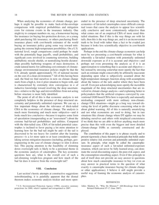
4. ics of climate change is the reduced-form relationship be-
tween atmospheric stocks of anthropogenically injected
CO2-e GHGs and temperature change. Instead of S1, which
stands for “climate sensitivity narrowly defined,” I work
throughout the rest of this paper with S2, which (abusing
scientific terminology somewhat here) stands for a more
abstract “generalized climate-sensitivity-like scaling param-
eter” that includes heat-induced feedbacks on the forcing
from the above-mentioned releases of naturally sequestered
GHGs, increased respiration of soil microbes, climate-
stressed forests, and other weakenings of natural carbon
sinks. The transfer from ⌬ ln [anthropogenically injected
CO2-e GHGs] to eventual ⌬T is not linear (and is not even
a true long-run equilibrium relationship), but for the pur-
poses of this highly aggregated example the linear approx-
imation is good enough. This suggests that a doubling of
anthropogenically injected CO2-e GHGs causes (very ap-
proximately) ultimate temperature change ⌬T ⬇ S2.
The main point here is that the PDF of S2 has an
even-longer, even-fatter tail than the PDF of S1. A recent
study by Torn and Harte (2006) can be used to give some
very rough idea of the relationship of the PDF of S2 to the
PDF of S1. It is universally accepted that in the absence of
any feedback gain, S1 ⫽ 1.2⬚C. If g1 is the conventional
feedback gain parameter associated with S1, then S1 ⫽
1.2/[1 ⫺ g1], whose inverse is g1 ⫽ [S1 ⫺ 1.2]/S1. Torn
and Harte estimated that heat-induced GHG releases add
about 0.067 of gain to the conventional feedback factor, so
that (expressed in my language) S2 ⫽ 1.2/[1 ⫺ g2], where
g2 ⫽ g1 ⫹ 0.067. (The 0.067 is only an estimate in a
linearized formula, but it is unclear in which direction
higher-order terms would pull the formula, and even if this
0.067 coefficient were considerably lower my point would
remain.) Doing the calculations, P[S1 ⬎ 7⬚C] ⫽ 5% ⫽
P[ g1 ⬎ 0.828] ⫽ P[ g2 ⬎ 0.895] implies P[S2 ⬎
11.5⬚C] ⫽ 5%. Likewise, P[S1 ⬎ 10⬚C] ⫽ 1% ⫽ P[ g1 ⬎
0.88] ⫽ P[ g2 ⬎ 0.947] implies P[S2 ⬎ 22.6⬚C] ⫽ 1%
and presumably corresponds to a scenario where CH4 and
CO2 are outgassed on a large scale from degraded perma-
frost soils, wetlands, and clathrates.5 The effect of heat-
induced GHG releases on the PDF of S2 is extremely
nonlinear at the upper end of the PDF of S2 because, so to
speak, “fat tails conjoined with fat tails beget yet-fatter
tails.”
Of course my calculations and the numbers above can be
criticized, but (quibbles and terminology aside) I don’t think
climate scientists would say these calculations are funda-
mentally wrong in principle or there exists a clearly superior
method for generating rough estimates of extreme-impact
tail probabilities. Without further ado I just assume for
purposes of this simplistic example that P[S2 ⬎ 10⬚C] ⬇
5% and P[S2 ⬎ 20⬚C] ⬇ 1%, implying that anthropogenic
doubling of CO2-e eventually causes P[⌬T ⬎ 10⬚C] ⬇ 5%
and P[⌬T ⬎ 20⬚C] ⬇ 1%, which I take as my base-case tail
estimates in what follows. These small probabilities of what
amounts to huge climate impacts occurring at some indef-
inite time in the remote future are wildly uncertain, unbe-
lievably crude ballpark estimates—most definitely not
based on hard science. But the subject matter of this paper
concerns just such kind of situations and my overly sim-
plistic example here does not depend at all on precise
numbers or specifications. To the contrary, the major point
of this paper is that such numbers and specifications must be
imprecise and that this is a significant part of the climate-
change economic-analysis problem, whose strong implica-
tions have thus far been ignored.
Stabilizing anthropogenically injected CO2-e GHG stocks
at anything like twice pre-industrial-revolution levels looks
now like an extremely ambitious goal. Given current trends
in emissions, we will attain such a doubling of anthropo-
genically injected CO2-e GHG levels around the middle of
this century and will then go far beyond that amount unless
drastic measures are taken starting soon. Projecting current
trends in business-as-usual GHG emissions, a tripling of
anthropogenically injected CO2-e GHG concentrations
would be attained relative to pre-industrial-revolution levels
by early in the 22nd century. Countering this effect is the
idea that we just might begin someday to seriously cut back
on GHG emissions (especially if we learn that a high-S2
catastrophe is looming—although the extraordinarily long
inertial lags in the commitment pipeline converting GHG
emissions into temperature increases might severely limit
this option). On the other hand, maybe currently underde-
veloped countries like China and India will develop and
industrialize at a blistering pace in the future with even
more GHG emissions and even less GHG emissions con-
trols than have thus far been projected. Or, who knows, we
might someday discover a revolutionary new carbon-free
energy source or make a carbon-fixing technological break-
through. Perhaps natural carbon-sink sequestration pro-
cesses will turn out to be weaker (or stronger) than we
thought. There is also the unknown role of climate engi-
neering. The recent scientific studies behind my crude
ballpark numbers could turn out to too optimistic or too
pessimistic—or I might simply be misapplying these num-
bers by inappropriately using values that are either too high
or too low. And so forth and so on. For the purposes of this
very crude example (aimed at conveying some very rough
empirical sense of the fatness of global-warming tails), I cut
5 I am grateful to John Harte for guiding me through these calculations,
although he should not be blamed for how I am interpreting or using the
numbers in what follows. The Torn and Harte study is based upon an
examination of the 420,000-year record from Antarctic ice cores of
temperatures along with associated levels of CO2 and CH4. While based
on different data and a different methodology, the study of Sheffer,
Brovkin, and Cox (2006) supports essentially the same conclusions as
Torn and Harte (2006). A completely independent study from simulating
an interactive coupled climate-carbon model of intermediate complexity
in Matthews and Keith (2007) confirms the existence of a strong carbon-
cycle feedback effect with especially powerful temperature amplifications
at high climate sensitivities.
THE REVIEW OF ECONOMICS AND STATISTICS
4

5. through the overwhelming enormity of climate-change un-
certainty and the lack of hard science about tail probabilities
by sticking with the overly simplistic story that P[S2 ⬎
10⬚C] ⬇ P[⌬T ⬎ 10⬚C] ⬇ 5% and P[S2 ⬎ 20⬚C] ⬇
P[⌬T ⬎ 20⬚C] ⬇ 1%. I can’t know precisely what these
tail probabilities are, of course, but no one can—and that is
the point here. To paraphrase again the overarching theme
of this example: the moral of the story does not depend on
the exact numbers or specifications in this drastic oversim-
plification, and if anything it is enhanced by the fantastic
uncertainty of such estimates.
It is difficult to imagine what ⌬T ⬇ 10⬚C–20°C might
mean for life on Earth, but such high temperatures have not
been seen for hundreds of millions of years and such a rate
of change over a few centuries would be unprecedented
even on a timescale of billions of years. Global average
warming of 10°C–20°C masks tremendous local and sea-
sonal variation, which can be expected to produce temper-
ature increases much greater than this at particular times in
particular places. Because these hypothetical temperature
changes would be geologically instantaneous, they would
effectively destroy planet Earth as we know it. At a mini-
mum such temperatures would trigger mass species extinc-
tions and biosphere ecosystem disintegration matching or
exceeding the immense planetary die-offs associated in
Earth’s history with a handful of previous geoenvironmental
mega-catastrophes. There exist some truly terrifying conse-
quences of mean temperature increases ⬇10°C–20°C, such
as disintegration of Greenland’s and at least the western part
of the Antarctic’s ice sheets with dramatic raising of sea
level by perhaps thirty meters or so, critically important
changes in ocean heat transport systems associated with
thermohaline circulations, complete disruption of weather,
moisture and precipitation patterns at every planetary scale,
highly consequential geographic changes in freshwater
availability, and regional desertification.
Alloftheabove-mentionedhorrifyingexamplesofclimate-
change mega-disasters are incontrovertibly possible on a
timescale of centuries. They were purposely selected to
come across as being especially lurid in order to drive home
a valid point. The tiny probabilities of nightmare impacts of
climate change are all such crude ballpark estimates (and
they would occur so far in the future) that there is a
tendency in the literature to dismiss altogether these highly
uncertain forecasts on the “scientific” grounds that they are
much too speculative to be taken seriously. In a classical-
frequentist mindset, the tiny probabilities of nightmare ca-
tastrophes are so close to 0 that they are highly statistically
insignificant at any standard confidence level, and one’s first
impulse can understandably be to just ignore them or wait
for them to become more precise. The main theme of this
paper contrasts sharply with the conventional wisdom of not
taking seriously extreme-temperature-change probabilities
because such probability estimates aren’t based on hard
science and are statistically insignificant. This paper shows
that the exact opposite logic holds by giving a rigorous
Bayesian sense in which, other things being equal, the more
speculative and fuzzy are the tiny tail probabilities of
extreme events, the less ignorable and the more serious is
the impact on present discounted expected utility for a
risk-averse agent.
Oversimplifying enormously here, how warm the climate
ultimately gets is approximately a product of two factors—
anthropogenically injected CO2-e GHGs and a critical
climate-sensitivity-like scaling multiplier. Both factors are
uncertain, but the scaling parameter is more open-ended
on the high side with a much longer and fatter upper tail.
This critical scale parameter reflecting huge scientific uncer-
tainty is then used as a multiplier for converting aggregated
GHG emissions—an input mostly reflecting economic
uncertainty—into eventual temperature changes. Suppose
the true value of this scaling parameter is unknown because
of limited past experience, a situation that can be modeled
as if inferences must be made inductively from a finite
number of data observations. At a sufficiently high level of
abstraction, each data point might be interpreted as repre-
senting an outcome from a particular scientific or economic
study. This paper shows that having an uncertain scale
parameter in such a setup can add a significant tail-fattening
effect to posterior-predictive PDFs, even when Bayesian
learning takes place with arbitrarily large (but finite)
amounts of data. Loosely speaking, the driving mechanism
is that the operation of taking “expectations of expectations”
or “probability distributions of probability distributions”
spreads apart and fattens the tails of the reduced-form
compounded posterior-predictive PDF. It is inherently dif-
ficult to learn from finite samples alone enough about the
probabilities of extreme events to thin down the bad tail of
the PDF because, by definition, we don’t get many data-
point observations of such catastrophes. The paper will
show that a generalization of this form of interaction can be
repackaged and analyzed at an even higher level of abstrac-
tion as an aggregative macroeconomic model with essen-
tially the same reduced form (structural uncertainty about
some unknown open-ended scaling parameter amplifying an
uncertain economic input). This form of interaction (cou-
pled with finite data, under conditions of everywhere-
positive relative risk aversion) can have very strong conse-
quences for CBA when catastrophes are theoretically
possible, because in such circumstances it can drive appli-
cations of EU theory much more than anything else, includ-
ing discounting.
When fed into an economic analysis, the great open-
ended uncertainty about eventual mean planetary tempera-
ture change cascades into yet much greater, yet much more
open-ended uncertainty about eventual changes in welfare.
There exists here a very long chain of tenuous inferences
fraught with huge uncertainties in every link beginning with
unknown base-case GHG emissions; then compounded by
huge uncertainties about how available policies and policy
THE ECONOMICS OF CATASTROPHIC CLIMATE CHANGE 5

6. levers transfer into actual GHG emissions; compounded by
huge uncertainties about how GHG-flow emissions accu-
mulate via the carbon cycle into GHG-stock concentrations;
compounded by huge uncertainties about how and when
GHG-stock concentrations translate into global mean tem-
perature changes; compounded by huge uncertainties about
how global mean temperature changes decompose into
regional temperature and climate changes; compounded by
huge uncertainties about how adaptations to, and mitiga-
tions of, climate-change damages are translated into utility
changes—especially at a regional level; compounded by
huge uncertainties about how future regional utility changes
are aggregated—and then how they are discounted—to
convert everything into expected-present-value global wel-
fare changes. The result of this immense cascading of huge
uncertainties is a reduced form of truly stupendous uncer-
tainty about the aggregate expected-present-discounted util-
ity impacts of catastrophic climate change, which mathe-
matically is represented by a very spread out, very fat-tailed
PDF of what might be called “welfare sensitivity.”
Even if a generalized climate-sensitivity-like scaling pa-
rameter such as S2 could be bounded above by some big
number, the value of “welfare sensitivity” is effectively
bounded only by some very big number representing some-
thing like the value of statistical civilization as we know it
or maybe even the value of statistical life on Earth as we
know it. This is the essential point of this simplistic moti-
vating example. Suppose it were granted for the sake of
argument that an abstract climate-sensitivity-like scaling
parameter such as S2 might somehow be constrained at the
upper end by some fundamental law of physics that assigns
a probability of exactly 0 to temperature change being above
some critical physical constant instead of continuously
higher temperatures occurring with continuously lower
probabilities trailing off asymptotically to 0. Even granted
such an upper bound on S2, the essential point here is that
the enormous unsureness about (and enormous sensitivity of
CBA to) an arbitrarily imposed “damages function” for high
temperature changes makes the relevant reduced-form cri-
terion of welfare sensitivity to a fat-tailed generalized scal-
ing parameter seem almost unbelievably uncertain at high
temperatures—to the point of being essentially unbounded
for practical purposes.
III. The Model
Let C be reduced-form consumption that has been ad-
justed for welfare by subtracting out all damages from
climate change. Adaptation and mitigation are considered to
be already included in C. Present consumption is normal-
ized as C0 ⬅ 1. Suppose to begin with that the represen-
tative agent has a standard familiar utility function of CRRA
(constant relative risk aversion) form
U共C兲 ⫽
C1⫺␩
1 ⫺ ␩
(1)
with coefficient ␩. Marginal utility is U⬘(C) ⫽ C⫺␩. Later
I consider non-CRRA utility.
For analytical crispness, the model of this paper has only
two periods—the present and the future. Applied to climate
change, I interpret the future as being very roughly about
two centuries hence. By using such a sharp formulation I
downplay the ability to learn and adapt gradually over time.
Likewise I repress the fact that higher ⌬T values are
correlated with later times of arrival. I argue subsequently in
the paper that key insights of this model will remain, mutatis
mutandis, when additional real-world complexities are lay-
ered on—including a more detailed specification of the
economics of climate change that incorporates learning
along with a realistically long inertial time lag from emitted
GHGs to eventual ⌬T. The main purpose of this paper is to
lay out the essential structure of my argument as simply as
possible, leaving more realistic refinements for later work.
Instead of working directly with future damages-adjusted
consumption C, in this paper it is more convenient to work
with (and think in terms of) ln C. If present consumption is
normalized to unity, then the growth of consumption be-
tween the two periods is
Y ⬅ ln C, (2)
where in this model Y is a random variable (RV) capturing
all uncertainty that influences future values of ln C, includ-
ing damages of adverse climate change. Throughout this
paper, Y encapsulates the reduced-form uncertainty that is at
the abstract core of an economic analysis of climate change:
the relationship between uncertain post-damages welfare-
adjusted C and uncertain ⌬T in the background. Thus, the
RV Y is to be interpreted as implicitly being some transfer
function of the RV ⌬T of form Y ⫽ F(⌬T), so that equation
(2) means C ⫽ exp(F(⌬T)). For simplicity, in this paper I
effectively take F(⌬T) to be of the linear form F(⌬T) ⫽
G ⫺ ␥⌬T with known positive constants G and ␥, but it
could be of the quadratic form F(⌬T) ⫽ G ⫺ ␥(⌬T)2 or of
many other forms. The essence of the structural-uncertainty
problem in the economics of climate change concerns the
process by which we come to understand underlying struc-
ture. Here one requires a model of how inductive knowledge
is acquired. This core issue is modeled starkly at a very high
reduced-form level of abstraction. I simply pretend the
inference mechanism is as if we learn the indirect effect of
⌬T on C via direct observations of past realizations of Y,
which are subsequently incorporated into a Bayesian-
updated reduced-form posterior-predictive PDF of Y.
With time-preference parameter ␤ (0 ⬍ ␤ ⱕ 1), the
“stochastic discount factor” or “pricing kernel” is
M共C兲 ⫽ ␤
U⬘共C兲
U⬘共1兲
⫽ ␤ exp共⫺␩Y兲. (3)
The amount of present consumption the agent would be
willing to give up in the present period to obtain one extra
THE REVIEW OF ECONOMICS AND STATISTICS
6

7. sure unit of consumption in the future period is E[M] ⫽
␤E[exp(⫺␩Y)], which is a kind of shadow price for dis-
counting future costs and benefits in project analysis.
Throughout the paper I use this price of a future sure unit of
consumption E[M] as the single most useful overall indi-
cator of the present cost of future uncertainty. Other like
indicators—such as welfare-equivalent deterministic con-
sumption or willingness to pay to avoid uncertainty—give
similar results, but the required analysis in terms of mean-
preserving spreads and so forth is slightly more elaborate
and slightly less intuitive. Focusing on the behavior of
E[M] is understood in this paper, therefore, as being a
metaphor for understanding what drives the results of all
utility-based welfare calculations in situations of potentially
unlimited exposure to catastrophic impacts.
Using standard notation, let lowercase y denote a realiza-
tion of the uppercase RV Y. If Y has PDF f( y), then
E关M兴 ⫽ ␤ 冕⫺⬁
⬁
e⫺␩y
f共y兲dy, (4)
which means that E[M] is essentially the Laplace transform
or moment-generating function (MGF) of f( y). Properties
of the expected stochastic discount factor are thus the same
as properties of the MGF of a PDF, about which a great deal
is already understood.
A prime example of equation (4) is the special case where
Y ⬃ N(␮, s2), which yields the familiar log normal formula
E关M兴 ⫽ exp冉⫺␦ ⫺ ␩␮ ⫹
1
2
␩2
s2
冊, (5)
where ␦ ⫽ ⫺ln ␤ is the instantaneous rate of pure time
preference. Equation (5) shows up in innumerable asset-
pricing Euler equation applications as the expected value of
the stochastic discount factor or pricing kernel when con-
sumption is log normally distributed. Expression (5) is also
the basis of the well-known generalized-Ramsey formula
for the risk-free interest rate
rf
⫽ ␦ ⫹ ␩␮ ⫺
1
2
␩2
s2
, (6)
which (in its deterministic form, for the special case s ⫽ 0)
plays a key role in recent debates about what social interest
rate to use for intergenerational cost-benefit discounting of
policies to mitigate GHG emissions. This intergenerational-
discounting debate has mainly revolved around choosing
“ethical” values of the rate of pure time preference ␦, but
this paper will demonstrate that, for any ␩ ⬎ 0, the effect of
␦ in formula (6) is theoretically overshadowed by the effect
of the uncertain scaling parameter s. It should be borne in
mind that equation (6) is an annuitized version of an
interest-rate formula being used here for discounting future
climate changes that will play itself out over a timescale of
two centuries or so.
To create families of probability distributions that are
simultaneously fairly general and analytically tractable, the
following generating mechanism is employed. Suppose Z
represents an RV normalized to have mean 0 and variance 1.
Let ␾(z) be any piecewise-continuous PDF satisfying
兰⫺⬁
⬁
z␾(z)dz ⫽ 0 and 兰⫺⬁
⬁
z2␾(z)dz ⫽ 1, where it should
be noted that the PDF ␾(z) is allowed to be extremely
general. For example, the distribution of Z might have finite
support (like the uniform distribution, which signifies that
unbounded catastrophes will be absolutely excluded condi-
tional on the value of the finite lower support being known),
or it might have unbounded range (like the normal, which
allows unbounded catastrophes to occur but assigns them a
thin bad tail conditional on the variance being known). The
only restrictions placed on ␾(z) are the weak regularity
conditions that ␾(z) ⬎ 0 within some neighborhood of z ⫽
0, and that E[exp(⫺␣z)] ⬍ ⬁ for all ␣ ⬎ 0, which is
automatically satisfied if Z has finite lower support.
With ␮ and s ⬎ 0 given, make the affine change of RV:
Y ⫽ sZ ⫹ ␮. The conditional PDF of y is then
h共 y兩s兲 ⫽
1
s
␾冉y ⫺ ␮
s
冊, (7)
where ␮, s are structural parameters having the interpreta-
tion: ␮ ⫽ E[Y], s2 ⫽ V[Y].
For this paper, what matters most is structural uncertainty
about the scale parameter controlling the tail spread of a
probability distribution, which is the most critical unknown
in this setup. This scale parameter s may be loosely con-
ceptualized as a highly stylized abstract generalization of a
climate-sensitivity-like amplifying or scaling multiplier
resembling S2. (In this crude analogy, Z 7 ⌬ ln CO2/ln 2,
SZ 7 ⌬T, Y 7 G ⫺ ␥⌬T.) Without significant loss of
generality, assume for ease of exposition that in equation (7)
the mean ␮ is known, while the standard-deviation scale
parameter s is unknown. The case where ␮ and s are both
unknown involves more intricate notation but otherwise
gives essentially identical results.
The point of departure here is that the conditional PDF of
growth rates h( y兩s) is given to the agent in the form of
equation (7) and, while the true value of s is unknown, the
situation is as if some finite number of i.i.d. observations are
available on which to base an estimate of s via some process
of inductive reasoning. Suppose that the agent has observed
the random sample y ⫽ ( y1, . . . , yn) of growth-rate data
realizations from n independent draws of the distribution
h( y兩s) defined by equation (7) for some unknown fixed
value of s. An example relevant to this paper is where the
sample space represents the outcomes of various economic-
scientific studies and the data y ⫽ ( y1, . . . , yn) are
interpreted at a very high level of abstraction as the findings
of n such studies. If we are allowed to make the further
abstraction that “inductive knowledge” is what we learn
THE ECONOMICS OF CATASTROPHIC CLIMATE CHANGE 7

8. from empirical data-evidence, then n here can be crudely
interpreted as a measure of the degree of inductive knowl-
edge of the situation.
The likelihood function is
L共s; y兲 ⬀ 写
j⫽1
n
h共yj兩s兲. (8)
Choose the prior PDF of S as
p0共s兲 ⬀ s⫺k
(9)
for some number k, crudely identifiable with the strength of
prior knowledge. As k can be chosen to be arbitrarily large,
the nondogmatic prior distribution (9) can be made to place
arbitrarily small prior probability weight on big values of s.
It should be appreciated that any scale-invariant prior must
be of the form (9). Scale invariance (discussed in the
Bayesian-statistical literature) is considered desirable as a
description of a “noninformative” reference or default prior
that favors no particular value of the scaling parameter s
over any other. For such a noninformative reference or
default prior, it seems not unreasonable to impose a condi-
tion of scale invariance from first principles. Suppose that
the action taken in any decision problem should not depend
upon the unit of measurement. Then the only prior consis-
tent with this plausible principle of scale invariance holding
over all possible decision problems must satisfy the condi-
tion p0(s) ⬀ p0(␣s), and the only way this can hold for all
␣ ⬎ 0, s ⬎ 0 is when the (necessarily improper) PDF has
form (9).
The posterior PDF pn(s兩y) is proportional to the prior
PDF p0(s) times the likelihood PDF L(s;y):
pn共s兩y兲 ⬀ p0共s兲 写
j⫽1
n
h共yj兩s兲. (10)
Integrating s out of equation (7), the unconditional or
marginal posterior-predictive PDF of y (to be plugged into
equation [4]) is
f共 y兲 ⫽ 冕0
⬁
h共 y兩s兲pn共s兩y兲ds. (11)
Consider the prototype specification: Z ⬃ N(0, 1);
Y兩␮, s ⬃ N(␮, s2); ␮ known; PDF of s is equation (10).
Sample variance is ␯n ⬅ 冘j⫽1
n
( yj ⫺ ␮)2/n. Any standard
textbook on Bayesian statistical theory indicates that, for
this prototype case, the posterior-predictive PDF (11) is the
Student-t
f共 y兲 ⬀ 冉1 ⫹
共 y ⫺ ␮兲2
n␯n
冊⫺共n⫹k兲/ 2
(12)
with n ⫹ k degrees of freedom. Asymptotically, the limiting
tail behavior of equation (12) is a fat-tailed power-law PDF
whose exponent is the sum of inductive plus prior knowl-
edge n ⫹ k.
When the posterior-predictive distribution of Y is equa-
tion (12) (from s being unknown), then equation (4) be-
comes
E关M兴 ⫽ ⫹⬁, (13)
because the MGF of a Student-t distribution is infinite.6
What accounts technically for the economically stunning
counterintuitiveness of the finding (13) is a form of point-
wise but nonuniform convergence. When n 3 ⬁ in equa-
tion (12), f( y) becomes the familiar normal form
exp(⫺( y ⫺ ␮)2/2␯⬁
2
), which then, as y 3 ⫺⬁, ap-
proaches 0 faster than exp(⫺␩y) approaches infinity,
thereby leading to the well-known finite formula (5) for
E[M]. Given any fixed n, on the other hand, as y 3 ⫺⬁
expression (12) tends to 0 only as fast as the power-law
polynomial (⫺y)⫺(n⫹k), so that now in formula (4) it is the
exponential term exp(⫺␩y) that dominates asymptotically,
thereby causing E[M] 3 ⫹⬁.
Something quite extraordinary seems to be happening
here, which is crying out for further elucidation! Thousands
of applications of EU theory in thousands of articles and
books are based on formulas like (5) or (6). Yet when it is
acknowledged that s is unknown (with a standard noninfor-
mative reference prior) and its value in formula (5) or (6)
must instead be inferred as if from a data sample that can be
arbitrarily large (but finite), expected marginal utility ex-
plodes. The question then naturally arises: What is EU
theory trying to tell us when its conclusions for a host of
important applications—in CBA, asset pricing, and many
other fields of economics—seem so sensitive merely to the
recognition that conditioned on finite realized data the
distribution implied by the normal is the Student-t?
The Student-t “child” posterior-predictive density from a
large number of observations looks almost exactly like its
bell-shaped normal “parent” except that the probabilities are
somewhat more stretched out, making the tails appear rel-
atively fatter at the expense of a slightly flatter center. In the
limit, the ratio of the fat Student-t tail probability divided by
the thin normal tail probability approaches infinity, even
while both tail probabilities are approaching 0. Intuitively, a
6 The example in this section with these particular functional forms
leading to existence problems from indefinite expected-utility integrals
blowing up was first articulated in the important pioneering note of
Geweke (2001). Weitzman (2007a) extended this example to a nonergodic
evolutionary stochastic process and developed some implications for asset
pricing in a nonstationary setting. For the application here to the econom-
ics of catastrophic climate change I believe the nonergodic evolutionary
formulation is actually more relevant and gives stronger insights, but it is
just not worth the additional complexity for what is essentially an applied
paper whose basic points are adequately conveyed by the simpler station-
ary case. The same comment applies to modeling the PDFs of S1, S2, or
⌬T in a less abstract way that ties the analysis more directly and more
specifically to the scientific climate-change literature as it stands now.
THE REVIEW OF ECONOMICS AND STATISTICS
8

9. normal density “becomes” a Student-t from a tail-fattening
spreading-apart of probabilities caused by the variance of
the normal having itself a (inverted gamma) probability
distribution. It is then no surprise from EU theory that
people are more averse qualitatively to a relatively fat-tailed
Student-t posterior-predictive child distribution than they
are to the relatively thin-tailed normal parent which begets
it. A perhaps more surprising consequence of EU theory is
the quantitative strength of this endogenously derived aver-
sion to the effects of unknown tail structure. The story
behind this quantitative strength is that fattened posterior-
predictive bad tails represent structural or deep uncertainty
about the possibility of rare high-impact disasters that—
using colorful language here—“scare” any agent having a
utility function with relative risk aversion everywhere
bounded above 0.
IV. The Key Role of a “VSL-Like Parameter”
To jump ahead of the story just a bit, last section’s general
model has essentially the same unsettling property as the
disturbing Normal 3 Student-t example given at the end of
the section—namely that E[M] is unbounded. The core
underlying problem is the difficulty of learning limiting tail
behavior inductively from finite data. Seemingly thin-tailed
probability distributions (like the normal), which are actu-
ally only thin-tailed conditional on known structural param-
eters of the model (like the standard deviation), become
tail-fattened (like the Student-t) after integrating out the
structural-parameter uncertainty. This core issue is generic
and cannot be eliminated in any clean way. When combined
with unlimited downside exposure it must influence any
utility function sensitive to low values of consumption.
Technically, for the analysis to proceed further some
mathematical mechanism is required to close the model in
the sense of bounding E[M]. A variety of bounding mech-
anisms are possible, with the broad general conclusions of
the model not being tied to any one particular bounding
mechanism. This paper closes the model by placing an ad
hoc positive lower bound on consumption, which is denoted
D (for “death”), so that always C ⱖ D ⬎ 0. The lower
bound D is not completely arbitrary, however, because it can
be related conceptually to a “fear of ruin” or a “value of
statistical life” (VSL) parameter.7 This has the advantage of
tying conclusions to a familiar economic concept whose
ballpark estimates can at least convey some extremely crude
quantitative implications for the economics of climate
change. In this empirical sense the glass is half full (which
is more than can be said for other ways of closing this
model). However, the glass is half empty in the empirical
sense that an accurate CBA of climate change can end up
being distressingly dependent on some very large VSL-like
coefficient about whose size we are highly unsure.
The critical coefficient that is behind the lower bound on
consumption is called the VSL-like parameter and is de-
noted ␭. This “VSL-like parameter” ␭ is intended to be akin
to the already somewhat vague concept of the value of a
human statistical life, only in the context here it represents
the yet far fuzzier concept of something more like the value
of statistical civilization as we know it, or perhaps even the
value of statistical life on Earth (as we know it). In this
paper I am just going to take ␭ to be some very big number
that indirectly controls the convergence of the integral
defining E[M] by implicitly generating a lower bound
D(␭) ⬎ 0 on consumption. An empirical first approxima-
tion of ␭ (normalized per capita) might be given by con-
ventional estimates of the value of a statistical human life,
which may be much too small for the purposes at hand but
will at least give some crude empirical idea of what is
implied numerically as a point of departure.
The basic idea is that a society trading off a decreased
probability of its own catastrophic demise against the cost
of lowering the probability of that catastrophe is facing a
decision problem conceptually analogous to how a person
might make a tradeoff between decreased consumption as
against a lower probability of that person’s own individually
catastrophic end. However artificial or peculiar the use of a
VSL-like parameter to close this model might seem in a
context of global climate change, other ways of closing this
model seem to me even more artificial or peculiar. I am not
trying to argue that a VSL-like parameter (as described
above) naturally and intuitively suggests itself as a great
candidate for closing this model—I am just saying that it
seems better than the alternatives. In this spirit, suppose for
the sake of developing the argument that the analysis is
allowed to proceed as if the treatment of the most cata-
strophic conceivable impact of climate change is very
roughly analogous to the simplest possible economic model
of the behavior of an individual agent who is trading off
increased consumption against a slightly increased proba-
bility of death.
Let D be a disastrously low value of consumption repre-
senting the analog of a starvation level, below which the
individual dies. Let the utility associated with death be
normalized at 0. The utility function U(C; D) is chosen to
be of the analytically convenient CRRA form
U共C; D兲 ⫽
C1⫺␩
⫺ D1⫺␩
1 ⫺ ␩
(14)
for C ⱖ D, and U(C; D) ⬅ 0 for 0 ⱕ C ⬍ D. The
constant CRRA coefficient in equation (14) is ␩.
7 The parameter ␭ that is being used here to truncate the extent of
catastrophic damages is akin to the “fear of ruin” coefficient introduced by
Aumann and Kurz (1977) to characterize an individual’s “attitude toward
risking his fortune” in binary lotteries. Foncel and Treich (2005) later
analyzed this fear-of-ruin coefficient and showed that it is basically the
same thing analytically as VSL. The particular utility function I use later
in this section is essentially identical (but with a different purpose in a
different context) to a specification used recently by Hall and Jones
(2007), which, according to them, is supported by being broadly consis-
tent with a wide array of stylized facts about health spending and
empirical VSL estimates.
THE ECONOMICS OF CATASTROPHIC CLIMATE CHANGE 9

10. Without loss of generality, current consumption is nor-
malized as it was before at C ⫽ 1. For simplicity, suppose
the agent begins with something close to a zero probability
of death in the current period. Let A(q) be the amount of
extra consumption the individual requires within this period
to exactly compensate for P[C ⱕ D] ⫽ q within this
period. In free translation, q is the probability of death.
From EU theory, A(q) satisfies the equation (1 ⫺ q)U(1 ⫹
A(q); D) ⬅ U(1; D), which, when differentiated with
respect to q and evaluated at q ⫽ 0 yields
⫺U共1; D兲 ⫹ U1共1; D兲␭ ⫽ 0, (15)
where ␭ ⬅ A⬘(0). Note that the “VSL-like parameter” ␭ is
defined as the rate of substitution between consumption and
mortality risk, here being A⬘(0).
Equation (15) can be inverted to give the implied lower
bound on consumption D as an implicit function of the
VSL-like parameter ␭. Inverting equation (15) for isoelastic
utility function (14) yields
D共␭兲 ⫽ 关1 ⫹ 共␩ ⫺ 1兲␭兴⫺1/共␩⫺1兲
. (16)
To ensure the reasonable condition that D(␭) in equation
(16) declines monotonically in ␭ requires that ␩ ⬎ 1, which
is hereby assumed.
From a wide variety of empirical studies in disparate
contexts, a plausible value of the coefficient of relative risk
aversion might be 2.8 Very rough ballpark estimates of the
per capita value of a statistical human life might be of the
order of magnitude of a hundred times per capita consump-
tion.9 Plugging ␩ ⬇ 2, ␭ ⬇ 100 into formula (16) gives
D(100) ⬇ 0.01. An interpretation of ␭ as a parameter
representing the per capita value of statistical civilization or
the per capita value of statistical life on Earth (as we
currently know or understand these concepts) presumably
involves much higher values of ␭ than ⬇100. Choosing, for
example, ␭ ⬇ 1,000 gives D(1,000) ⬇ 0.001. In any
event, I note here for later reference that a Monte Carlo
simulation assessing the EU impacts of losing up to 99%
(much less 99.9%) of welfare-equivalent consumption in
the bad fat tail is very different from any simulations now
being done with any existing empirical model of climate
change.
V. The Dismal Theorem
Let E[M兩␭] represent the expected value of a stochastic
discount factor M(C) given by formula (3) when C ⱖ D(␭)
(or, equivalently, Y ⱖ ln D(␭)) and given by M(C) ⫽
(D(␭))⫺␩ when C ⬍ D(␭) (or, equivalently, Y ⬍ ln D(␭)),
where D(␭) is defined by equation (16). The following
“dismal theorem” (hereafter sometimes abbreviated “DT”)
shows under quite general circumstances what happens to
the price of future consumption E[M兩␭] when ␭ might be
very big.
Theorem 1. For any given n and k,
lim
␭3⬁
E关M兩␭兴 ⫽ ⫹⬁. (17)
Proof. Combining the interpretation of D(␭) from equa-
tion (16) with equations (4) and (11)—and tracing the links
of equations from (16) all the way back to (7)—implies that
E关M兩␭兴 ⬀ 冕0
⬁
1
sk⫹n⫹1 写
j⫽1
n
␾冉yj ⫺ ␮
s
冊
(18)
⫻ 冋冕lnD共␭兲
⬁
e⫺␩y
␾冉y ⫺ ␮
s 冊dy册ds.
Make the change of variable z ⫽ ( y ⫺ ␮)/s, use the fact
from equation (16) that D(⬁) ⫽ 0, and reverse the order of
integration to rewrite equation (18) as
lim
␭3⬁
E关M兩␭兴
⬀ 冕⫺⬁
⬁
␾共z兲冋冕0
⬁
e⫺␩zs
1
sk⫹n 写
j⫽1
n
␾冉yj ⫺ ␮
s 冊ds册dz.
(19)
Pick any value of z⬘ for which simultaneously z⬘ ⬍ 0 and
␾(z) ⬎ 0 in an open neighborhood of z ⫽ z⬘. Then note
that
lim
s3⬁
再e⫺␩z⬘s
1
sk⫹n冎⫽ ⫹⬁, (20)
implying equation (19) also approaches ⫹⬁ as ␭ 3 ⬁,
which concludes this proof sketch.10 ■
8 Two is the point estimate for ␩ selected by Hall and Jones (2007) in a
conceptually similar model and defended by them with references to a
wide range of studies on page 61 of their paper.
9 For this particular application of using a VSL-like parameter to analyze
the extent of the worst imaginable climate-change catastrophe, I think that
the most one might hope for is accuracy to within about an order of
magnitude—anything more being false precision. Even the empirical
estimates for the value of a much better defined statistical human life have
a disturbingly wide range, but ␭ ⬇ 100 is roughly consistent with the
meta-analysis in Bellavance, Dionne, and Lebeau (2007) or the survey of
Viscusi and Aldy (2003).
10 This is only a highly compressed, loose sketch of the structure of a
proof. It is being included here primarily to provide some motivation for
the formulas in the analysis, which comes next, that depend upon equation
(20). In this spirit, the purpose of this “proof sketch” is to give at least a
minimal quick-and-dirty indication of where equation (20) is coming
from. A rigorous proof can be built around the very significant (perhaps
even seminal) contribution of Michael Schwarz to decision-making under
extreme uncertainty. An important result proved in Schwarz (1999) is that,
in the limit, the tails of f( y) defined by equation (11) are power-law of
order n ⫹ k. From this fact, a rigorous proof of theorem 1 then proceeds
along the lines sketched here.
THE REVIEW OF ECONOMICS AND STATISTICS
10

11. The underlying logic behind the strong result of theorem
1 is described by the limiting behavior of equation (20) for
large values of s. Given any values of n and k, the proba-
bility of a disaster declines polynomially in the scale s of the
disaster from equation (20), while the marginal-utility im-
pact of a disaster increases exponentially in the scale s of
the disaster. It is intuitive, and can readily be proved, that
the tail of the RV Y essentially behaves like the tail of the
RV S. Therefore, irrespective of the original parent distri-
bution, the effect of an uncertain scale parameter fattens the
tail of the posterior-predictive child distribution so that it
behaves asymptotically like a power-law distribution with
coefficient from equation (20) equal to n ⫹ k. In this sense,
power-law tails need not be postulated, because they are
essentially unavoidable in posterior-predictive PDFs.11 No
matter the (finite) number of observations, the race to the
bottom of the bad tail between a polynomially contracting
probability times an exponentially expanding marginal-
utility impact is won in the limit every time by the marginal-
utility impact—for any utility function having positive rel-
ative risk aversion in the limit as C 3 0⫹. This point is
important: utility isoelasticity per se is inessential to the
reasoning here (although it makes the argument easier to
understand), because the expected stochastic discount fac-
tor E[M] 3 ⫹⬁ in this setup for any relatively risk-
averse utility function satisfying the curvature require-
ment inf
C⬎0
[⫺CU⬙(C)/U⬘(C)] ⬎ 0.
I want to emphasize emphatically: the key issue here is
not a mathematically illegitimate use of the symbol ⫹⬁ in
formulas (13) or (17), which incorrectly seems to offer a
deceptively easy way out of the dilemma that E[M] 3 ⫹⬁
by somehow discrediting this application of EU theory on
the narrow grounds that infinities are not allowed in a
legitimate theory of choice under uncertainty. It is easy to
put arbitrary bounds on utility functions, to truncate prob-
ability distributions arbitrarily, or to introduce ad hoc priors
that arbitrarily cut off or otherwise severely dampen high
values of S or low values of C. Introducing any of these
changes formally closes the model in the sense of replacing
the symbol ⫹⬁ by an arbitrarily large but finite number.
Indeed, the model of this paper has been closed in just such
a fashion by placing a lower bound on consumption of the
form C ⱖ D, where the lower bound D(␭) ⬎ 0 is defined
indirectly by a “value of statistical life” parameter ␭. How-
ever, removing the infinity symbol in this or any other way
does not eliminate the underlying problem because it then
comes back to haunt in the form of an arbitrarily large
expected stochastic discount factor, whose exact value de-
pends sensitively upon obscure bounds, truncations, se-
verely dampened or cut-off prior PDFs, or whatever other
tricks have been used to banish the ⫹⬁ symbol. One can
easily remove the ⫹⬁ in formulas (13) or (17), but one
cannot so easily remove the underlying economic problem
that expected stochastic discount factors—which lie at the
heart of cost-benefit, asset-pricing, and many other impor-
tant applications of EU theory—can become arbitrarily
large just from unobjectionable statistical inferences about
limiting tail behavior. The take-away message here is that
reasonable attempts to constrict the length or the fatness of
the “bad” tail (or to modify the utility function) still can
leave us with uncomfortably big numbers whose exact value
depends nonrobustly upon artificial constraints or parame-
ters that we really do not understand. The only legitimate
way to avoid this potential problem is when there exists
strong a priori knowledge that restrains the extent of total
damages. If a particular type of idiosyncratic uncertainty
affects only one small part of an individual’s or a society’s
overall portfolio of assets, exposure is naturally limited to
that specific component and bad-tail fatness is not such a
paramount concern. However, some very few but very
important real-world situations have potentially unlimited
exposure due to structural uncertainty about their potentially
open-ended catastrophic reach. Climate change potentially
affects the whole worldwide portfolio of utility by threat-
ening to drive all of planetary welfare to disastrously low
levels in the most extreme scenarios.
The interpretation and application of theorem 1 is sensi-
tive to a subtle but important behind-the-scene tug of war
between pointwise but nonuniform limiting behavior in ␭
and pointwise but nonuniform limiting behavior in n. This
kind of bedeviling nonuniform convergence haunts fat-
tailed CBA and turns numerical climate-change applications
of DT into a practical nightmare. To see more clearly how
the issue of determining E[M] under pointwise but nonuni-
form convergence plays itself out, suppose that, unbe-
knownst to the agent, the “true” value of s is s*. Since the
prior p0(s) by equation (9) assigns positive probability to an
open interval around s*, the imposed specification has
sufficient regularity for large-sample likelihood dominance
to cause strong (that is, almost sure) convergence of the
posterior distribution (10) of S to its true data-generating
process (DGP) value s ⫽ s*. This in turn means that the
posterior-predictive PDF of growth rates (11) converges
strongly to its true DGP distribution h( y兩s*) and—for any
given ␭ ⬍ ⬁—E[M兩␭] converges strongly to its true value:
n 3 ⬁ f E关M兩␭兴 O
¡
a.s.
␤ 冕⫺⬁
⬁
e⫺␩y
1
s*
␾ 冉y ⫺ ␮
s*
冊dy. (21)
Condition (21) signifies that for any given ␭ ⬍ ⬁ (which
via equation [16] puts a positive lower bound D(␭) on C,
11 As stated here, DT depends upon an invariant prior of the polynomial
(aka power-law aka Pareto) form (9), but this is not much of a limitation
because k can be any number. To undo the infinite limit in (17) requires a
noninvariant prior that additionally approaches 0 faster than any polyno-
mial in 1/s (as s 3 ⬁). In such a case the limit in (17) is a finite number,
but its (potentially arbitrarily large) value will depend critically upon the
strong a priori knowledge embodied in the presumed-known parameters
of such a noninvariant prior—and the prior-sensitivity message that such
a formulation ends up delivering is very similar anyway to the message
delivered by the model of this paper.
THE ECONOMICS OF CATASTROPHIC CLIMATE CHANGE 11

12. and thereby a finite upper bound on M), in the limit as full
structural knowledge is approached (because n 3 ⬁),
E[M兩␭] goes to its true value. What is happening here is that
as the strength of inductive knowledge n is increasing in the
form of more and more data observations piling up, it is
becoming increasingly apparent that the probability of C
being anywhere remotely as low as the cutoff D(␭) is
ignorable—even after taking into account the possible EU
impacts of disastrously low utilities for C close to D(␭). A
conventional pure-risk-like application of thin-tailed EU
theory essentially corresponds, then, to a situation where
there is sufficient inductive-plus-prior knowledge to identify
the relevant structure because n ⫹ k is reasonably large
relative to the VSL-like parameter ␭—and relative to the
much less controversial parameters ␤ and ␩.
Concerning conventional parameters ␤ and ␩, we have at
least some rough idea of what might be empirically relevant
(say ␤ ⬇ 99% per year and ␩ ⬇ 2). In complete contrast,
any discussion about climate change concerning the empir-
ically relevant value of the nonconventional VSL-like pa-
rameter ␭ belongs to a much more abstract realm of dis-
course. It is therefore understandable to want climate-
change CBA to be restricted to dealing only with modest
damages by disregarding nightmare scenarios (as being “too
speculative” or “not based on hard science”) via chopping
off the really-bad tail and then ignoring it. This is the de
facto strategy employed by most of those relatively few
existing CBAs of climate change that even bother to con-
cern themselves at all with a formal treatment of uncertain
high-impact damages. Alas, to be confident in the validity of
such a cutoff strategy in a situation where we are grossly
unsure about ␭ or D effectively requires uniform conver-
gence of E[M] for all conceivable values of ␭ or D.
Otherwise, for any given level of inductive-plus-prior
knowledge n ⫹ k, a skeptical critic could always come back
and ask how robust is CBA to the highly unsure truncation
value of D(␭). Similar robustness questions apply to any a
priori presumption or imposition of thin-tailed PDFs.
Note well that with equation (21) the a.s. convergence of
E[M兩␭] to its true value is pointwise but not uniform in n.
No matter how much data-evidence n exists—or even can
be imagined to exist—DT says that E[M兩␭] is always
exceedingly sensitive to very large values of ␭. If “risk”
means that the DGP is known exactly (only the outcome is
random), while “uncertainty” means that (as well as the
outcome being random) the parameters of the DGP are
unknown and must be estimated statistically, then DT can be
interpreted as saying that structural “uncertainty” can al-
ways trump pure “risk” for situations of potentially unlim-
ited downside exposure when no plausible bound D(␭) ⬎ 0
can confidently be imposed by prior knowledge. DT can
therefore be interpreted as implying a spirit in which it may
be unnecessary to append to the theory of decision-making
under uncertainty an ad hoc extra postulate of “ambiguity
aversion.” At least for situations where there is fundamental
uncertainty about an open-ended catastrophe coexisting
with fear of ruin, EU theory itself already tells us precisely
how the “ambiguity” of structural-parameter uncertainty
can be especially important and why people may be much
more averse to it than to pure objective-frequency “risk.”
The dismal theorem makes a general point but also has a
particular application to the economics of climate change.
The general point is that theorem 1 embodies a very strong
form of a “generalized precautionary principle” for situa-
tions of potentially unlimited downside exposure. From
experience alone one cannot acquire sufficiently accurate
information about the probabilities of disasters in the bad
tail to make E[M] or E[U] independent of the VSL-like
parameter ␭—thereby potentially allowing this VSL-like-
parameter aspect to dominate CBA applications of EU
theory under conditions of potentially unlimited liability.
The part of the distribution of possible future outcomes
that can most readily be learned (from inductive information
of a form as if conveyed by data) concerns the relatively
more likely outcomes in the middle of the distribution. From
previous experience, past observations, plausible interpola-
tions or extrapolations, and the law of large numbers, there
may be at least some modicum of confidence in being able
to construct a reasonable picture of the central regions of the
posterior-predictive PDF. As we move toward probabilities
in the periphery of the distribution, however, we are increas-
ingly moving into the unknown territory of subjective un-
certainty where our probability estimate of the probability
distributions themselves becomes increasingly diffuse be-
cause the frequencies of rare events in the tails cannot be
pinned down by previous experiences or past observations.
It is not possible to learn enough about the frequency of
extreme tail events from finite samples alone to make E[M]
or E[U] independent of artificially imposed bounds on the
extent of possibly ruinous disasters. This principle is true
even in the stationary model of this paper where an ergodic
theorem holds, but it applies much more forcefully to an
evolutionary process like real-world anthropogenic warm-
ing.12 Climate-change economics generally—and the fat-
ness of climate-sensitivity tails specifically—are prototype
examples of this principle, because we are trying to extrap-
olate inductive knowledge far outside the range of limited
past experience.
VI. What Is the Dismal Theorem Trying to Tell Us?
A common reaction to the conundrum for CBA implied
by DT is to acknowledge its mathematical logic but to
wonder how it is to be used constructively for deciding what
to do in practice. Is DT an economics version of an impos-
sibility theorem which signifies that there are fat-tailed
situations where economic analysis is up against a very
12 This principle comes across with much greater force in an evolution-
ary world based upon an analytically more complicated nonstationary
nonergodic stochastic process modeled along the lines of Weitzman
(2007a).
THE REVIEW OF ECONOMICS AND STATISTICS
12

13. strong constraint on the ability of any quantitative analysis
to inform us without committing to a VSL-like parameter
and an empirical CBA framework that is based upon some
explicit numerical estimates of the miniscule probabilities
of all levels of catastrophic impacts down to absolute
disaster? Even if it were true that DT represents a valid
economic-statistical precautionary principle which, at least
theoretically, might dominate decision-making, would not
putting into practice this “generalized precautionary princi-
ple” freeze all progress if taken too literally? Considering
the enormous inertias that are involved in the buildup of
GHGs, and the warming consequences, is the possibility of
learning and mid-course corrections a plausible counter-
weight to DT, or, at the opposite extreme, has the commit-
ment of GHG stocks in the ultra-long pipeline already
fattened the bad tail so much that it doesn’t make much
difference what is done in the near future about GHG
emissions? How should the bad fat tail of climate uncer-
tainty be compared with the bad fat tails of various proposed
solutions such as nuclear power, geoengineering, or carbon
sequestration in the ocean floor? Other things being equal,
the dismal theorem suggests as a policy response to climate
change a relatively more cautious approach to GHG emis-
sions, but how much more caution is warranted?
I simply do not know the full answers to the extraordi-
narily wide range of legitimate questions that DT raises. I
don’t think anyone does. But I also don’t think that such
questions can be allowed in good conscience to be simply
brushed aside by arguing, in effect, that when probabilities
are small and imprecise, then they should be set precisely to
0. To the extent that uncertainty is formally considered at all
in the economics of climate change, the artificial practice of
using thin-tailed PDFs—especially the usual practice of
imposing de minimis low-probability-threshold cutoffs that
casually dictate what part of the high-impact bad tail is to be
truncated and discarded from CBA—seems arbitrary and
problematic.13 In the spirit that the unsettling questions
raised by fat-tailed CBA for the economics of climate
change must be addressed seriously, even while admitting
that we do not now know all of the answers, I offer here
some speculative thoughts on what it all means. Even if the
quantitative magnitude of what DT implies for climate-
change policy seems somewhat hazy, the qualitative direc-
tion of the policy advice is nevertheless quite clear.
Any interpretation or application of the dismal theorem is
rendered exceedingly tricky by the bedeviling (for CBA)
nonuniform convergence of E[M] or E[U] in its other
parameters relative to the key VSL-like parameter ␭. This
nonuniform convergence enables E[M] or E[U] to explode
(for any other given parameter values) as ␭ 3 ⬁. One might
try to argue that the values of E[M] or E[U] are ultimately
an empirical matter to be decided empirically (by analytical
formulas or simulation results), with relevant parameter
values of ␭, n, k, ␦, ␩, ␮, and so forth being taken together
as an empirically plausible ensemble. The idea that the
values of E[M] or E[U] should depend on testable, empir-
ically reasonable values of ␭ and the other parameters is, of
course, right on some level—and it sounds reassuring. Yet,
as a practical matter, the fact that E[M] and E[U] are so
sensitive to large values of ␭ (or small values of D), about
which we can have little confidence in our own a priori
knowledge, casts a very long shadow over any empirical
CBA of a situation to which the dismal theorem might
apply. In ordinary, limited-exposure or thin-tailed situations,
there is at least the underlying theoretical reassurance that
finite-cutoff-based CBA might (at least in principle) be an
arbitrarily close approximation to something that is accurate
and objective. In fat-tailed, unlimited-exposure DT situa-
tions, by contrast, there is no such theoretical assurance
underpinning the arbitrary cutoffs, which is ultimately due
to the haunting lack of uniform convergence of E[M] or
E[U] with respect to ␭ or D.
One does not want to abandon lightly the ideal that CBA
should bring independent empirical discipline to any appli-
cation by being based upon empirically reasonable param-
eter values. Even when DT applies, CBA based upon em-
pirically reasonable functional forms and parameter values
(including ␭) might reveal useful information. Simulta-
neously one does not want to be obtuse by insisting that DT
per se makes no practical difference for CBA because the
VSL-like coefficient ␭ is just another parameter to be
determined empirically and then simply plugged into the
analysis along with some extrapolative guesses about the
form of the “damages function” for high-temperature catas-
trophes (combined with speculative extreme-tail probabili-
ties). So a tricky balance is required between being over-
awed by DT into abandoning CBA altogether and being
underawed by DT into insisting that it is just another
empirical issue to be sorted out by business-as-usual CBA.
The degree to which the kind of “generalized precaution-
ary principle” embodied in the dismal theorem is relevant
for a particular application must be decided on a case-by-
case “rule of reason” basis. It depends generally upon the
extent to which prior ␭-knowledge and prior k-knowledge
combine with inductive-posterior n-knowledge in a partic-
ular case to fatten or to thin the bad tail. In the particular
application to the economics of climate change, with so
obviously limited data and limited experience about the
catastrophic reach of climate extremes, to ignore or suppress
the significance of rare fat-tailed disasters is to ignore or
suppress what economic-statistical decision theory is telling
us here loudly and clearly is potentially the most important
part of the analysis.
Where does global warming stand in the portfolio of
extreme risks currently facing us? There exist maybe half a
dozen or so serious “nightmare scenarios” of environmental
disasters perhaps comparable in conceivable worst-case
13 Adler (2007) sketches out in some detail the many ways in which de
minimis low-probability-threshold cutoffs are arbitrary and problematic in
more ordinary regulatory settings.
THE ECONOMICS OF CATASTROPHIC CLIMATE CHANGE 13

14. impact to catastrophic climate change. These might include
biotechnology, nanotechnology, asteroids, strangelets, pan-
demics, runaway computer systems, and nuclear prolifera-
tion.14 It may well be that each of these possibilities of
environmental catastrophe deserves its own CBA applica-
tion of DT along with its own empirical assessment of how
much probability measure is in the extreme tails around
D(␭). Even if this were true, however, it would not lessen
the need to reckon with the strong potential implications of
DT for CBA in the particular case of climate change.
Perhaps it is little more than raw intuition, but for what it
is worth I do not feel that the handful of other conceivable
environmental catastrophes are nearly as critical as climate
change. I illustrate with two specific examples. The first is
widespread cultivation of crops based on genetically mod-
ified organisms (GMOs). At casual glance, climate-change
catastrophes and bioengineering disasters might look simi-
lar. In both cases, there is deep unease about artificial
tinkering with the natural environment, which can generate
frightening tales of a planet ruined by human hubris. Sup-
pose for specificity that with GMOs the overarching fear of
disaster is that widespread cultivation of so-called Franken-
food might somehow allow bioengineered genes to escape
into the wild and wreak havoc on delicate ecosystems and
native populations (including, perhaps, humans), which
have been fine-tuned by millions of years of natural selec-
tion. At the end of the day I think that the potential for
environmental disaster with Frankenfood is much less than
the potential for environmental disaster with climate
change—along the lines of the following loose and over-
simplified reasoning.
In the case of Frankenfoods interfering with wild organ-
isms that have evolved by natural selection, there is at least
some basic underlying principle that plausibly dampens
catastrophic jumping of artificial DNA from cultivars to
landraces. After all, nature herself has already tried endless
combinations of mutated DNA and genes over countless
millions of years, and what has evolved in the fierce battle
for survival is only an infinitesimal subset of the very fittest
permutations. In this regard there exists at least some
inkling of a prior high-k argument making it fundamentally
implausible that Frankenfood artificially selected for traits
that humans find desirable will compete with or genetically
alter the wild types that nature has selected via Darwinian
survival of the fittest. Wild types have already experienced
innumerable small-step genetic mutations, which are per-
haps comparable to large-step human-induced artificial
modifications and which have not demonstrated survival
value in the wild. Analogous arguments may also apply for
invasive “superweeds,” which so far represent a minor
cultivation problem lacking ability to displace either land-
races or cultivars. Besides all this, safeguards in the form of
so-called terminator genes can be inserted into the DNA of
GMOs, which directly prevent GMO genes from reproduc-
ing themselves.
A second possibly relevant example of comparing climate
change with another potential catastrophe concerns the
possibility of a large asteroid hitting Earth. In the asteroid
case it seems plausible to presume there is much more
high-n inductive knowledge (from knowing something
about asteroid orbits and past collision frequencies) pinning
down the probabilities to very small “almost known” values.
If we use P[⌬T ⬎ 20⬚C] ⬇ 1% as the very rough proba-
bility of a climate-change cataclysm occurring within the
next two centuries, then this is roughly 10,000 times larger
than the probability of a large asteroid impact (of a one-in-
a-hundred-million-years size) occurring within the same
time period.
Contrast the above discussion about plausible magnitudes
or probabilities of disaster for genetic engineering or aster-
oid collisions with possibly catastrophic climate change.
The climate-change “experiment,” whose eventual outcome
we are trying to infer now, “tests” the planet’s response to a
geologically instantaneous exogenous injection of GHGs.
An exogenous injection of this much GHGs this fast seems
unprecedented in Earth’s history stretching back perhaps
billions of years. Can anyone honestly say now, from very
limited low-k prior information and very limited low-n
empirical experience, what are reasonable upper bounds on
the eventual global warming or climate change that we are
currently trying to infer will be the outcome of such a
first-ever planetary experiment? What we do know about
climate science and extreme tail probabilities is that planet
Earth hovers in an unstable trigger-prone “whipsaw” ocean-
atmosphere system,15 chaotic dynamic responses to geolog-
ically instantaneous GHG shocks are quite possible, and all
22 recently published studies of climate sensitivity cited by
IPCC-AR4 (2007), when mechanically aggregated together,
estimate on average that P[S1 ⬎ 7⬚C] ⬇ 5%. To my mind
this open-ended aspect with a way-too-high subjective prob-
ability of a catastrophe makes GHG-induced global climate
change vastly more worrisome than cultivating Frankenfood
or colliding with large asteroids.
These two examples hint at making a few meaningful
distinctions among the handful of situations where DT
might reasonably apply. My discussion here is hardly con-
clusive, so we cannot rule out a biotech or asteroid disaster.
However, I would say on the basis of this line of argument
that such disasters seem extremely unlikely, whereas a
climate disaster seems “only” very unlikely. In the language
of this paper, synthetic biology or large asteroids feel more
like high-(k ⫹ n) situations that we know a lot more about
relative to climate change, which by comparison feels more
like a low-(k ⫹ n) situation about which we know rela-
tively little. Regardless of whether my argument here is
convincing, the overarching principle is this: the mere fact
14 Many of these are discussed in Posner (2004), Sunstein (2007), and
Parson (2007).
15 On the nature of this unstable “whipsaw” climate equilibrium, see
Hansen et al. (2007).
THE REVIEW OF ECONOMICS AND STATISTICS
14

15. that DT might also apply to a few other environmental
catastrophes does not constitute a valid reason for excluding
DT from applying to climate change.
The simplistic two-period setup of this paper ignores or
suppresses some important features of the climate-change
problem. For instance, the really high values of ⌬T are more
likely to arrive (if they arrive at all) at further-distant future
times. A more careful model of temperature dynamics16
shows that the flavor of the two-period model survives this
over-simplification via the following intuitive logic. If ␶ is
the time of possible arrival of really high values of ⌬T, then
distant-future ␶ is associated with low ␤ in formula (4), and
once again we have the bedeviling (for CBA) existence of
pointwise but nonuniform convergence—here in ␭ and ␶ (or
␭ and ␤). For any given ␭ ⬍ ⬁, ␶ 3 ⬁ implies ␤ 3 0, which
in equation (4) implies E[M] 3 0. But for any given ␤ ⬎
0, from DT ␭ 3 ⬁ implies E[M] 3 ⬁. Again here, this
nonuniform-convergence aspect of the problem is what
turns fat-tailed CBA into such an empirical-numerical night-
mare for the economic evaluation of climate change.
A simplistic two-period setup also represses the real-
option value of waiting and learning. Concerning this as-
pect, however, with climate change we are on the four horns
of two dilemmas. The horns of the first dilemma are the twin
facts that built-up stocks of GHGs might end up ex post
representing a hugely expensive irreversible accumulation,
but so too might massive investments in noncarbon tech-
nologies that are at least partly unnecessary.
The second dilemma is the following. Because climate-
change catastrophes develop slower than some other poten-
tial catastrophes, there is ostensibly somewhat more chance
for learning and mid-course corrections with global warm-
ing relative to, say, biotechnology (but not necessarily
relative to asteroids when a good tracking system is in
place). The possibility of “learning by doing” may well be
a more distinctive feature of global-warming disasters than
some other disasters, and in that sense deserves to be part of
an optimal climate-change policy. The other horn of this
second dilemma, however, is the nasty fact that the ultimate
climate response to GHGs has tremendous inertial pipeline-
commitment lags of several centuries (via the carbon cycle).
When all is said and done, I don’t think there is a smoking
gun in the biotechnology, asteroid, or any other catastrophe
scenario quite like the idea that a crude amalgamation of
numbers from the most recent peer-reviewed published
scientific articles is suggesting something like P[S2 ⬎
10⬚C] ⬇ 5% and P[S2 ⬎ 20⬚C] ⬇ 1%.
Global climate change unfolds over a timescale of cen-
turies and, through the power of compound interest, a
standard CBA of what to do now to mitigate GHGs is
hugely sensitive to the discount rate that is postulated. This
has produced some sharp disagreements among economists
about what is an “ethical” value of the rate of pure time
preference ␦ (and the CRRA coefficient ␩) to use for
intergenerational discounting in the deterministic version
(s ⫽ 0) of the Ramsey equation (6) that forms the analytical
backbone for most studies of the economics of climate
change.17 For the model of this paper, which is based on
structural uncertainty, arguments about what values of ␦ to
use in equations (5) or (6) translate into arguments about
what values of ␤ to use in the model’s structural-uncertainty
generalization of the Ramsey equation (4). (A zero rate of
pure time preference ␦ ⫽ 0 in equation [6] corresponds to
␤ ⫽ 1 in equation [4].) In this connection, theorem 1 seems
to be saying that no matter what values of ␤ or ␩ are
selected, so long as ␩ ⬎ 0 and ␤ ⬎ 0 (equivalent to ␦ ⬍ ⬁),
any big-␭ CBA of GHG-mitigation policy should be pre-
sumed (until shown otherwise empirically) to be affected by
fat-tailed structural uncertainty. The relevance of this pre-
sumption is brought home starkly by a simple numerical
example based on equations (14) and (16) that if ␭ ⬇ 1,000
and the probability of a life-ending catastrophe is ⬇0.005,
then for ␩ ⬇ 2 the (undiscounted) willingness to pay to
avoid this catastrophe is ⬇83% of consumption.
Expected utility theory in the form of DT seems to be
suggesting here that the debate about discounting may be
secondary to a debate about the open-ended catastrophic
reach of climate disasters. While it is always fair game to
challenge the assumptions of a model, when theory provides
a generic result (like “free trade is Pareto optimal” or
“steady growth eventually outstrips one-time change”) the
burden of proof is commonly taken as being upon whoever
wants to overrule the theorem in a particular application.
The burden of proof in climate-change CBA is presump-
tively upon whoever calculates expected discounted utilities
without considering that structural uncertainty might matter
more than discounting or pure risk. Such a middle-of-the-
distribution modeler should be prepared to explain why the
bad fat tail of the posterior-predictive PDF does not play a
significant role in climate-change CBA when it is combined
with a specification that assigns high disutility to high
temperatures.
VII. Possible Implications for Climate-Change Policy
A so-called integrated assessment model (hereafter
“IAM”) for climate change is a multiequation computerized
model linking aggregate economic growth with simple cli-
mate dynamics to analyze the economic impacts of global
16 Available upon request as Weitzman, “Some Dynamic Implications of
the Climate-Sensitivity Inference Problem” (2008).
17 While this contentious intergenerational-discounting issue has long
existed (see, for example, the various essays in Portney & Weyant, 1999),
it has been elevated to recent prominence by publication of the contro-
versial Stern Review of the Economics of Climate Change (2007). The
Review argues for a base case of preference-parameter values ␦ ⬇ 0 and
␩ ⬇ 1, on which its strong conclusions depend analytically. Alternative
views of intergenerational discounting are provided in, for example,
Dasgupta (2007), Nordhaus (2007), and Weitzman (2007b). The last of
these also contains a heuristic exposition of the contents of this paper, as
well as giving Stern some credit for emphasizing informally the great
uncertainties associated with climate change.
THE ECONOMICS OF CATASTROPHIC CLIMATE CHANGE 15

16. warming. An IAM is essentially a dynamic model of an
economy with a controllable GHG-driven externality of
endogenous greenhouse warming. IAMs have proven them-
selves useful for understanding some aspects of the eco-
nomics of climate change—especially in describing out-
comes from a complicated interplay of the very long lags
and huge inertias involved. Most existing IAMs treat central
forecasts of damages as if they were certain and then do
some sensitivity analysis on parameter values. In the rare
cases where an IAM formally incorporates uncertainty, it
uses thin-tailed PDFs including, especially, truncation of
PDFs at arbitrary cutoffs. With the model of this paper,
uncertainty about adaptation and mitigation shows up in the
reduced form of a fat-tailed PDF of Y ⬅ ln C. In the IAM
literature, this issue of very unsure adaptation and mitiga-
tion involves discussion or even debate about the appropri-
ate choice of a deterministic “damages function” for high-
temperature changes.
All existing IAMs treat high-temperature damages by an
extremely casual extrapolation of whatever specification is
arbitrarily assumed to be the low-temperature “damages
function.” High-temperature damages extrapolated from a
low-temperature damages function are remarkably sensitive
to assumed functional forms and parameter combinations
because almost anything can be made to fit the low-
temperature damages assumed by the modeler. Most IAM
damages functions reduce welfare-equivalent consumption
by a quadratic-polynomial multiplier equivalent to 1/[1 ⫹
␥(⌬T)2], with ␥ calibrated to some postulated loss for
⌬T ⬇ 2⬚C–3°C. There was never any more compelling
rationale for this particular loss function than the comfort
that economists feel from having worked with it before. In
other words, the quadratic-polynomial specification is used
to assess climate-change damages for no better reason than
casual familiarity with this particular form from other cost-
of-adjustment dynamic economic models, where it has been
used primarily for analytical simplicity.
I would argue that if, for some unfathomable reason,
climate-change economists want dependence of damages
to be a function of (⌬T)2, then a far better function at
high temperatures for a consumption-reducing, welfare-
equivalent, quadratic-based multiplier is the exponential
form exp(⫺␥(⌬T)2). Why? Look at the specification
choice abstractly. What might be called the “temperature
harm” to welfare is arriving here as the arbitrarily imposed
quadratic form H(⌬T) ⫽ (⌬T)2, around which some fur-
ther structure is built to convert into utility units. With
isoelastic utility, the exponential specification is equivalent
to dU/U ⬀ dH, while for high H the polynomial specifi-
cation is equivalent to dU/U ⬀ dH/H. For me it is obvious
that, between the two, the former is much superior to the
latter. When temperatures are already high in the latter case,
why should the impact of dH on dU/U be artificially and
unaccountably diluted via dividing dH by high values of H?
The same argument applies to any polynomial in ⌬T. I
cannot prove that my favored choice is the more reasonable
of the two functional forms for high ⌬T (although I truly
believe that it is), but no one can disprove it either—and this
is the point here.
The value of ␥ required for calibrating welfare-equivalent
consumption at ⌬T ⬇ 2⬚C–3°C to be (say) ⬇ 97%–98% of
consumption at ⌬T ⫽ 0⬚C is so miniscule that both the
polynomial-quadratic multiplier 1/[1 ⫹ ␥(⌬T)2] and the
exponential-quadratic multiplier exp(⫺␥(⌬T)2) give virtu-
ally identical outcomes for relatively small values of ⌬T ⱕ
5⬚C, but at ever higher temperatures they gradually, yet ever
increasingly, diverge. With a fat-tailed PDF of ⌬T and a
very large value of the VSL-like parameter ␭, there can be
a big difference between these two functional forms in the
implied willingness to pay (WTP) to avoid or reduce un-
certainty in ⌬T. When the consumption-reducing, welfare-
equivalent damages multiplier has the exponential form
exp(⫺␥(⌬T)2), then as the VSL-like parameter ␭ 3 ⬁, a
DT-type argument for ␩ ⬎ 1 implies in the limit that the
WTP to avoid (or even reduce) fat-tailed uncertainty ap-
proaches 100% of consumption. This does not mean, of
course, that we should be spending 100% of consumption to
eliminate the climate-change problem.
But this limiting example does highlight how a damages
specification more reactive to high temperatures (than the
standard multiplicative-in-consumption polynomial-quadratic
specification) can dominate climate-change CBA when it is
combined with fat tails.
A further issue with IAMs is that samplings based upon
conventional Monte Carlo simulations of the economics of
climate change may give a very misleading picture of the
EU consequences of alternative GHG-mitigation policies.18
The core problem is that while it might be true in expecta-
tions that utility-equivalent damages of climate change are
enormous, when chasing a fat tail this will not be true for the
overwhelming bulk of Monte Carlo realizations. DT can be
approached by a Monte Carlo simulation only as a double
limit where the grid-range and the number of runs both go
to infinity simultaneously. To see this in a crisp thought
experiment, imagine what would happen to the simple
stripped-down model of this paper in the hands of a Monte
Carlo IAM simulator.
A finite grid may not reveal the true expected stochastic
discount factor or true expected discounted utility in simu-
lations of this model (even in the limit of an infinite number
of runs) because the most extreme negative impacts in the
fattened tails will have been truncated and evaluated at but
a single point representing an artificially imposed lower
bound on the set of all possible bad outcomes from all
conceivable negative impacts. Such arbitrarily imposed de
18 Tol (2003) showed the empirical relevance of this issue in some actual
IAM simulations. I am grateful to Richard Carson for suggesting the
inclusion of an explicit discussion of why a Monte Carlo simulation may
fail to account fully for the implications of uncertain large impacts with
small probabilities.
THE REVIEW OF ECONOMICS AND STATISTICS
16

17. minimis threshold-cutoff truncations are typically justified
(when anyone bothers to justify them at all) on the thin-
tailed frequentist logic that probabilities of extremely rare
events are statistically insignificantly different from 0—and
hence can be ignored. This logic might conceivably suffice
for known thin tails, but the conclusion is highly erroneous
for the rare and unusual class of fat-tailed potentially high-
impact economic problems to which climate change seem-
ingly belongs. Back-of-the-envelope calculations cited ear-
lier in this paper appear to indicate that a Monte Carlo
simulation of the economics of climate change requires
seriously probing into the implications of disastrous tem-
peratures and catastrophic impacts in incremental steps that
might conceivably cause up to a 99% (or maybe even much
greater) decline of welfare-equivalent consumption before
the modeler is allowed to cut off the rest of the bad fat tail
in good conscience and discard it. This paper says that any
climate-change IAM that does not go out on a limb by
explicitly committing to a Monte Carlo simulation that
includes the ultra-miniscule but fat-tailed probabilities of
super-catastrophic impacts (down to 1%, or even consider-
ably less, of current welfare-equivalent consumption) is in
possible violation of best-practice economic analysis be-
cause (by ignoring the extreme tails) it could constitute a
serious misapplication of EU theory. The policy relevance
of any CBA coming out of such a thin-tail-based model
might then remain under a very dark cloud until this fat-tail
issue is addressed seriously and resolved empirically.19
Additionally, a finite sample of Monte Carlo simulations
may not reveal true expected utility in this model (even in
the limit of an infinite grid) because the restricted sample
may not be able to go deep enough into the fat tails where
the most extreme damages are. Nor will typical sensitivity
analysis necessarily penetrate sufficiently far into the fat-tail
region to represent accurately the EU consequences of
disastrous damages. For any IAM (which presumably has a
core structure resembling the model of this paper), special
precautions are required to ensure that Monte Carlo simu-
lations represent accurately the low-utility impacts of fat-
tailed PDFs by having the grid-range and the number of
runs both be very large.
Instead of the existing IAM emphasis on estimating or
simulating economic impacts of the more plausible climate-
change scenarios, to at least compensate partially for finite-
sample bias the model of this paper calls for a dramatic
oversampling of those stratified climate-change scenarios
associated with the most adverse imaginable economic
impacts in the bad fat tail. With limited sampling resources
for the big IAMs, Monte Carlo analysis could be used much
more creatively—not necessarily to defend a specific policy
result, but to experiment seriously in order to find out more
about what happens with fat-tailed uncertainty and signifi-
cant high-temperature damages in the limit as the grid size
and number of runs increase simultaneously. Of course this
emphasis on sampling climate-change scenarios in propor-
tion to utility-weighted probabilities of occurrence forces us
to estimate subjective probabilities down to extraordinarily
tiny levels and also to put degree-of-devastation weights on
disasters with damage impacts up to perhaps being welfare-
equivalent to losing 99% (or possibly even more) of con-
sumption—but that is the price we must be willing to pay
for having a genuine economic analysis of potentially cat-
astrophic climate change.
In situations of potentially unlimited damage exposure
like climate change, it might be appropriate to emphasize a
slightly better treatment of the worst-case fat-tail ex-
tremes—and what might be done about them, at what
cost—relative to refining the calibration of most-likely out-
comes or rehashing point estimates of discount rates (or
climate sensitivity). A clear implication of this paper is that
greater research effort is relatively ineffectual when targeted
at estimating central tendencies of what we already know
relatively well about the economics of climate change in the
more plausible scenarios. A much more fruitful goal of
research might be to aim at understanding even slightly
better the deep uncertainty (which potentially permeates the
economic analysis) concerning the less plausible scenarios
located in the bad fat tail. I also believe that an important
complementary research agenda, which stems naturally
from the analysis of this paper, is the desperate need to
comprehend much better all of the options for dealing with
high-impact climate-change extremes. This should include
undertaking well-funded detailed studies and experiments
about the feasibility, deleterious environmental side effects,
and cost-effectiveness of geoengineering options to slim
down the bad fat tail quickly as part of emergency prepared-
ness for runaway climate situations if things are beginning
to slip out of hand—even while acknowledging that geo-
engineering might not be appropriate as a first-line defense
against greenhouse warming.20
19 Several back-of-the-envelope numerical examples, available upon
request, indicate to my own satisfaction that the fat-tail effect is likely to
be significant for at least some reasonable parameter values and functional
forms. However, serious IAM-based numerical simulations of fat-tail
effects on the economics of climate change have not yet been done and are
more properly the subject of another more empirical study and paper.
20 With the unfortunately limited information we currently possess,
geoengineering via injection into the stratosphere of sulfate aerosol
precursors or other artificially constructed particulates looks superficially
like it may be a cheap and effective way to slim down the bad fat tail of
high temperatures quickly as an emergency response—although with
largely unknown and conceivably nasty unintended consequences that we
need to understand much better. For more on the economics and politics
of geoengineering (with further references), see, for example, Barrett
(2007). In my opinion there is an acute, even desperate, need for a more
pragmatic, more open-minded approach to the prospect of climate engi-
neering—along with much more extensive research on (and experimen-
tation with) various geoengineering options for dealing with potential
runaway climate change. This research should include studying more
seriously and open-mindedly the possible bad side effects on the environ-
ment of geoengineering and everything else, as part of a cost-benefit-
effectiveness assessment of climate-change strategies that honestly in-
cludes the pluses and minuses of all actual policy alternatives and
tradeoffs that we realistically face on climate-change options.
THE ECONOMICS OF CATASTROPHIC CLIMATE CHANGE 17

18. When analyzing the economics of climate change, per-
haps it might be possible to make back-of-the-envelope
comparisons with empirical probabilities and mitigation
costs for extreme events in the insurance industry. One
might try to compare numbers on, say, a homeowner buying
fire insurance (or buying fire-protection devices, or a young
adult purchasing life insurance, or others purchasing flood-
insurance plans) with cost-benefit estimates of the world
buying an insurance policy going some way toward miti-
gating the extreme high-temperature possibilities. On a U.S.
national level, rough comparisons could perhaps be made
with the potentially huge payoffs, small probabilities, and
significant costs involved in countering terrorism, building
antiballistic missile shields, or neutralizing hostile dictator-
ships possibly harboring weapons of mass destruction. A
crude natural metric for calibrating cost estimates of climate-
change environmental-insurance policies might be that the
U.S. already spends approximately 3% of national income
on the cost of a clean environment.21 All of this having been
said, the bind we find ourselves in now on climate change
starts from a high-␭, low-k prior situation to begin with, and
is characterized by extremely slow convergence in n of
inductive knowledge toward resolving the deep uncertain-
ties—relative to the lags and irreversibilities from not acting
before structure is more fully identified.
The point of all of this is that economic analysis is not
completely helpless in the presence of deep structural un-
certainty and potentially unlimited exposure. We can say a
few important things about the relevance of thick-tailed
CBA to the economics of climate change. The analysis is
much more frustrating and much more subjective—and it
looks much less conclusive—because it requires some form
of speculation (masquerading as an “assessment”) about the
extreme bad-fat-tail probabilities and utilities. Compared
with the thin-tailed case, CBA of fat-tailed potential catas-
trophes is inclined to favor paying a lot more attention to
learning how fat the bad tail might be and—if the tail is
discovered to be too heavy for comfort after the learning
process—is a lot more open to at least considering under-
taking serious mitigation measures (including, perhaps, geo-
engineering in the case of climate change) to slim it down
fast. This paying attention to the feasibility of slimming
down overweight tails is likely to be a perennial theme in
the economic analysis of catastrophes. The key economic
questions here are, what is the overall cost of such a
tail-slimming weight-loss program and how much of the
bad fat does it remove from the overweight tail?
VIII. Conclusion
Last section’s heroic attempts at constructive suggestions
notwithstanding, it is painfully apparent that the dismal
theorem makes economic analysis trickier and more open-
ended in the presence of deep structural uncertainty. The
economics of fat-tailed catastrophes raises difficult concep-
tual issues that cause the analysis to appear less scientifi-
cally conclusive and more contentiously subjective than
what comes out of an empirical CBA of more usual thin-
tailed situations. But if this is the way things are with fat
tails, then this is the way things are, and it is an inconvenient
truth to be lived with rather than a fact to be evaded just
because it looks less scientifically objective in cost-benefit
applications.
Perhaps in the end the climate-change economist can help
most by not presenting a cost-benefit estimate for what is
inherently a fat-tailed situation with potentially unlimited
downside exposure as if it is accurate and objective—and
perhaps not even presenting the analysis as if it is an
approximation to something that is accurate and objective—
but instead by stressing somewhat more openly the fact that
such an estimate might conceivably be arbitrarily inaccurate
depending upon what is subjectively assumed about the
high-temperature damages function along with assumptions
about the fatness of the tails and/or where they have been
cut off. Even just acknowledging more openly the incredible
magnitude of the deep structural uncertainties that are in-
volved in climate-change analysis—and explaining better to
policymakers that the artificial crispness conveyed by con-
ventional IAM-based CBAs here is especially and unusually
misleading compared with more ordinary non-climate-
change CBA situations—might go a long way toward ele-
vating the level of public discourse concerning what to do
about global warming. All of this is naturally unsatisfying
and not what economists are used to doing, but in rare
situations like climate change where DT applies we may be
deluding ourselves and others with misplaced concreteness
if we think that we are able to deliver anything much more
precise than this with even the biggest and most detailed
climate-change IAMs as currently constructed and de-
ployed.
The contribution of this paper is to phrase exactly and to
present rigorously a basic theoretical principle that holds under
positive relative risk aversion and potentially unlimited expo-
sure. In principle, what might be called the catastrophe-
insurance aspect of such a fat-tailed unlimited-exposure
situation, which can never be fully learned away, can dom-
inate the social-discounting aspect, the pure-risk aspect, and
the consumption-smoothing aspect. Even if this principle in
and of itself does not provide an easy answer to questions
about how much catastrophe insurance to buy (or even an
easy answer in practical terms to the question of what
exactly is catastrophe insurance buying for climate change
or other applications), I believe it still might provide a
useful way of framing the economic analysis of catastro-
phes.
REFERENCES
Adler, Matthew D., “Why De Minimis?” AEI-Brookings Joint Center
Related Publication 07-17 (June 2007).
21 U.S. Environmental Protection Agency (1990), executive summary
projections for 2000, which I updated and extrapolated to 2007.
THE REVIEW OF ECONOMICS AND STATISTICS
18

19. Allen, Myles R., and David J. Frame, “Call Off the Quest,” Science 318
(October 26, 2007), 582–583.
Aumann, Robert J., and Mordecai Kurz, “Power and Taxes,” Economet-
rica 199 (1977), 1137–1161.
Barrett, Scott, “The Incredible Economics of Geoengineering,” Johns
Hopkins mimeograph (March 18, 2007).
Bellavance, Francois, Georges Dionne, and Martin Lebeau, “The Value of
a Statistical Life: A Meta-Analysis with a Mixed Effects Regres-
sion Model,” HEC Montreal working paper no. 06-12 (January 7,
2007).
Dasgupta, Partha, “Commentary: The Stern Review’s Economics of Cli-
mate Change,” National Institute Economic Review 199 (2007),
4–7.
Foncel, Jerome, and Nicolas Treich, “Fear of Ruin,” The Journal of Risk
and Uncertainty 31 (2005), 289–300.
Geweke, John, “A Note on Some Limitations of CRRA Utility,” Econom-
ics Letters 71 (2001), 341–345.
Hansen, James, et al., “Climate Change and Trace Gases,” Phil. Trans. R.
Soc. A 365 (2007), 1925–1954.
Hall, Robert E., and Charles I. Jones, “The Value of Life and the Rise in
Health Spending,” Quarterly Journal of Economics 122 (2007),
39–72.
IPCC-AR4, Climate Change 2007: The Physical Science Basis. Contri-
bution of Working Group I to the Fourth Assessment Report of the
Intergovernmental Panel on Climate Change (New York: Cam-
bridge University Press, 2007). Available online at http://www.
ipcc.ch.
Matthews, H. Damon, and David W. Keith, “Carbon-Cycle Feedbacks
Increase the Likelihood of a Warmer Future,” Geophysical Re-
search Letters 34 (2007), L09702.
Nordhaus, William D., “The Stern Review on the Economics of Climate
Change,” Journal of Economic Literature 45:3 (2007), 686–702.
Parson, Edward A., “The Big One: A Review of Richard Posner’s
Catastrophe: Risk and Response,” Journal of Economic Literature
XLV (March 2007), 147–164.
Portney, Paul R., and John P. Weyant (Eds.), Discounting and Intergen-
erational Equity (Washington, DC: Resources for the Future,
1999).
Posner, Richard A., Catastrophe: Risk and Response (New York: Oxford
University Press, 2004).
Roe, Gerard H., and Marcia B. Baker, “Why Is Climate Sensitivity So
Unpredictable?” Science 318 (October 26, 2007), 629–632.
Schwarz, Michael, “Decision Making Under Extreme Uncertainty,” Stan-
ford University Graduate School of Business, PhD dissertation
(1999).
Sheffer, Martin, Victor Brovkin, and Peter M. Cox, “Positive Feedback
between Global Warming and Atmospheric CO2 Concentration
Inferred from Past Climate Change,” Geophysical Research Letters
33:10 (2006), L10702.
Stern, Nicholas, et al., The Economics of Climate Change (New York:
Cambridge University Press, 2007).
Sunstein, Cass R., Worst-Case Scenarios (Cambridge, MA: Harvard
University Press, 2007).
Tol, Richard S. J., “Is the Uncertainty about Climate Change Too Large for
Expected Cost-Benefit Analysis?” Climatic Change 56 (2003),
265–289.
Torn, Margaret S., and John Harte, “Missing Feedbacks, Asymmetric
Uncertainties, and the Underestimation of Future Warming,” Geo-
physical Research Letters 33:10 (2006), L10703.
U.S. Environmental Protection Agency, Environmental Investments: The
Cost of a Clean Environment (Washington, DC: U.S. Government
Printing Office, 1990).
Viscusi, W. Kip, and Joseph E. Aldy, “The Value of a Statistical Life: A
Critical Review of Market Estimates throughout the World,” Jour-
nal of Risk and Uncertainty 5 (2003), 5–76.
Weitzman, Martin L., “Subjective Expectations and Asset-Return Puz-
zles,” American Economic Review 97:4 (2007a), 1102–1130.
“The Stern Review of the Economics of Climate Change,”
Journal of Economic Literature 45:3 (2007b), 703–724.
THE ECONOMICS OF CATASTROPHIC CLIMATE CHANGE 19