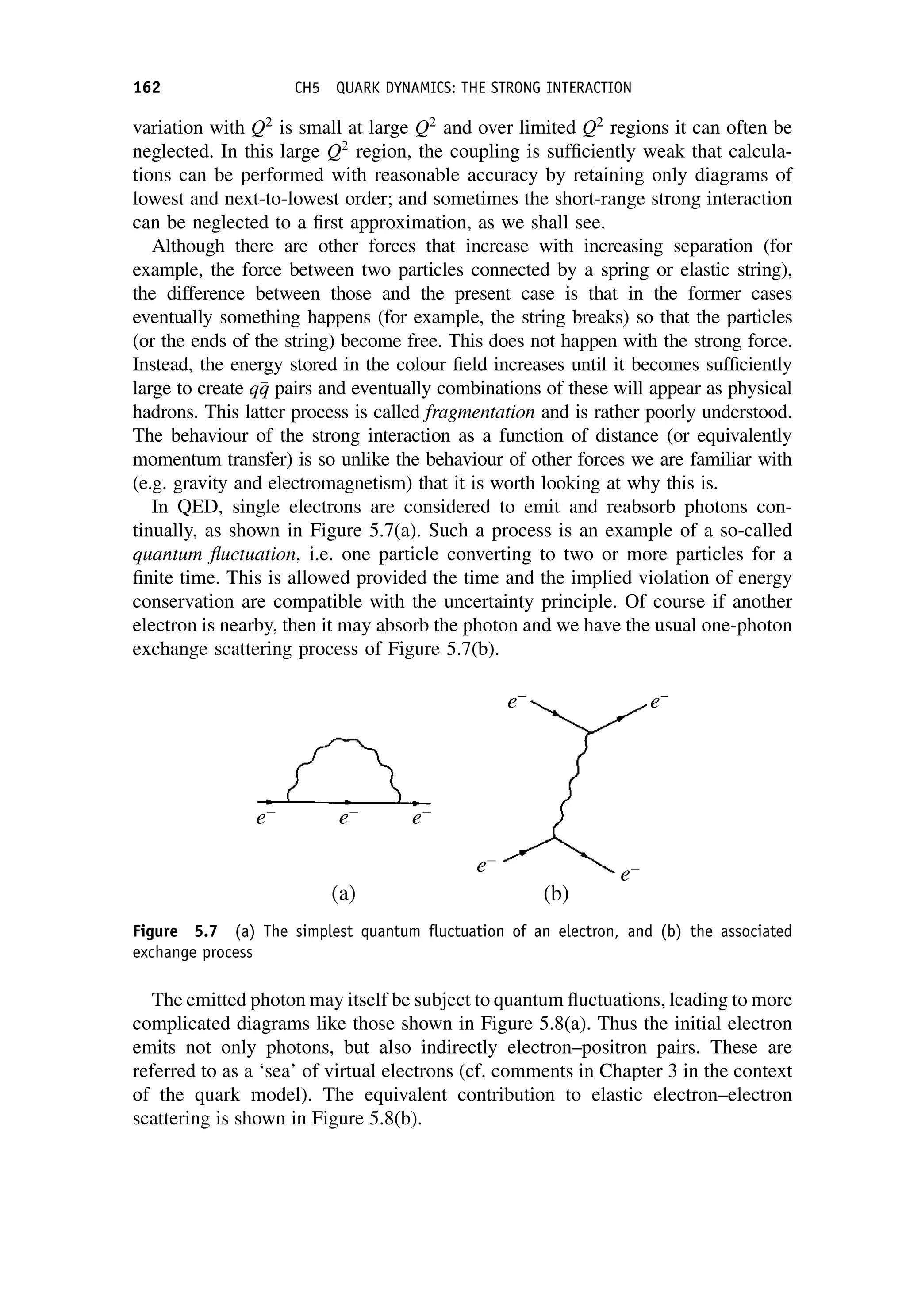
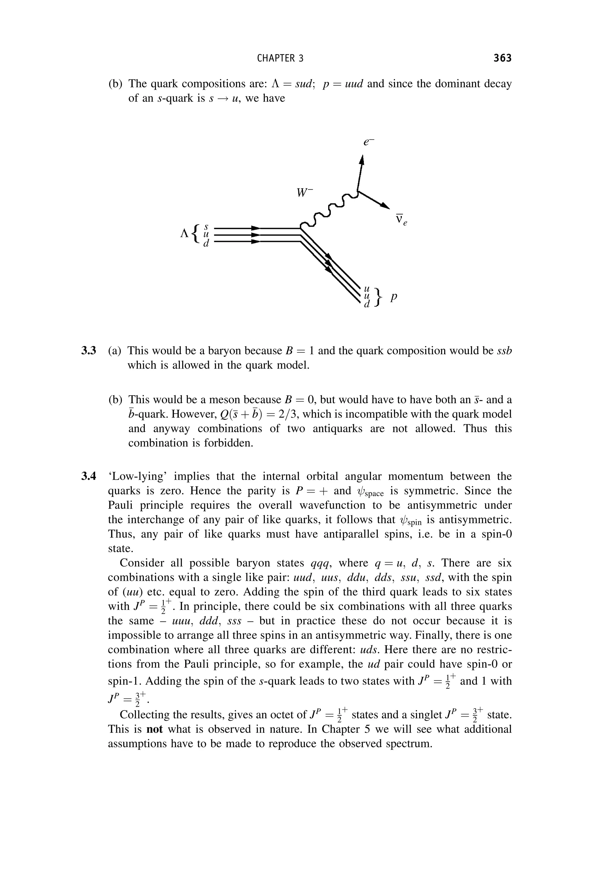
Download to read offline
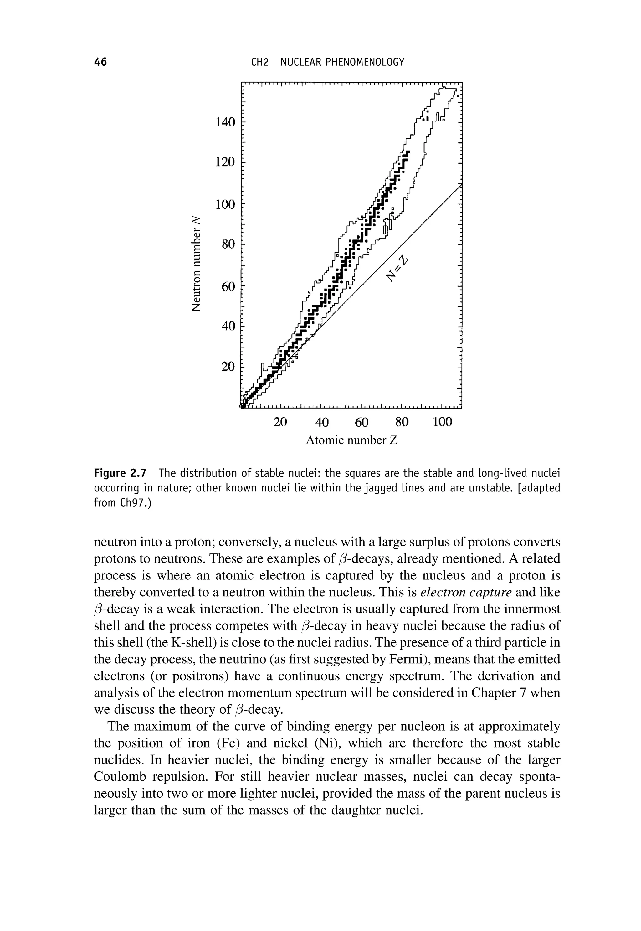
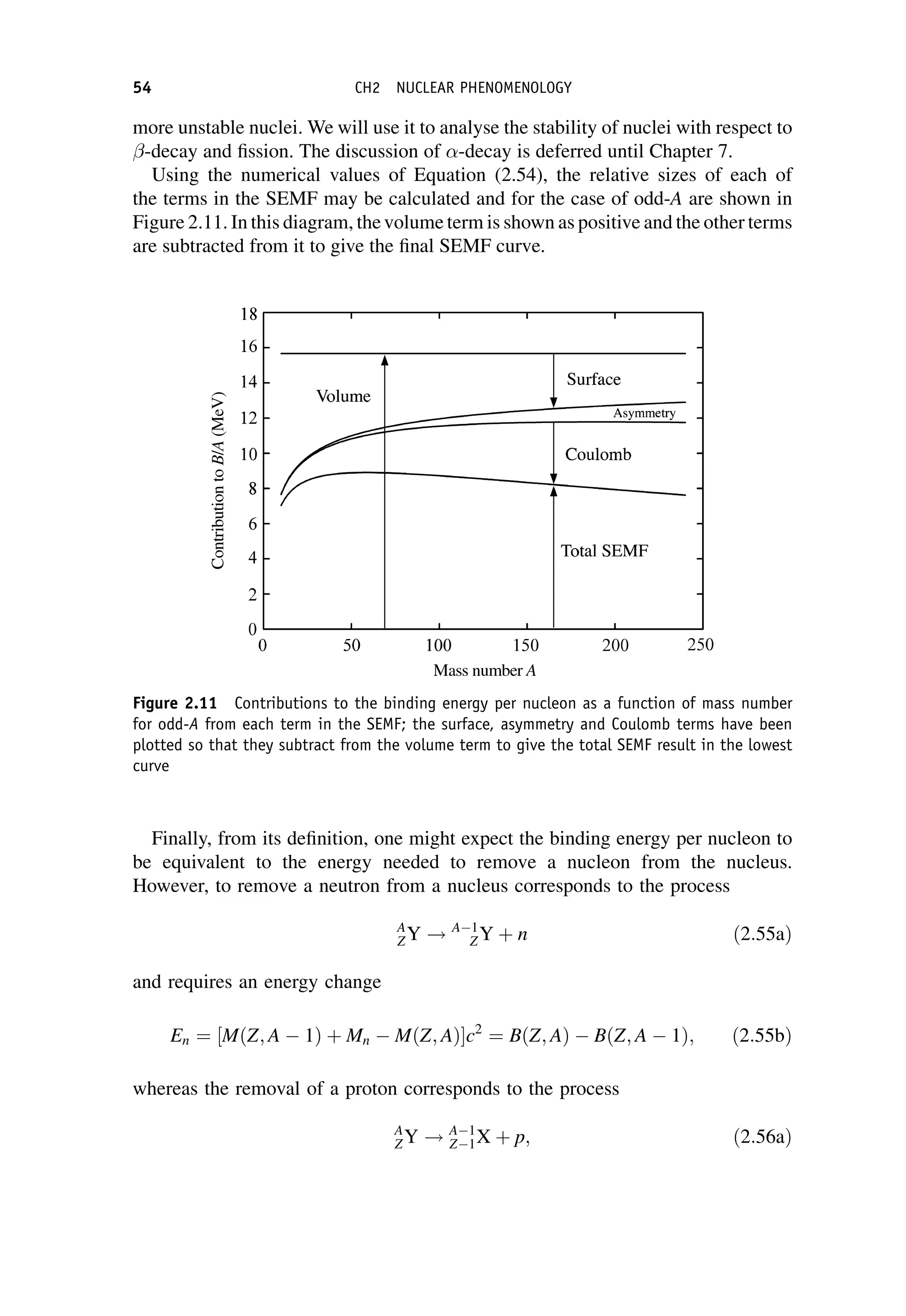

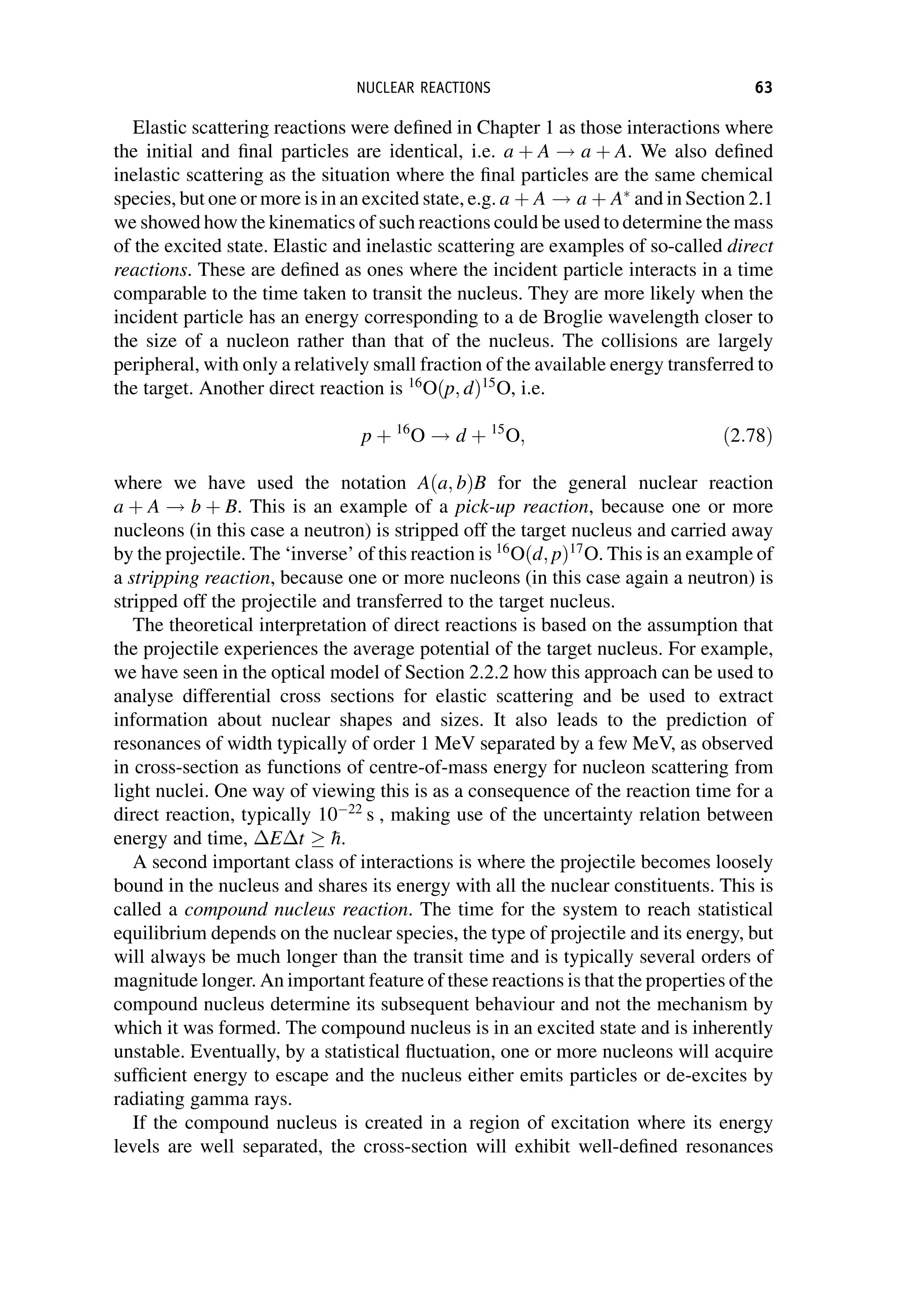

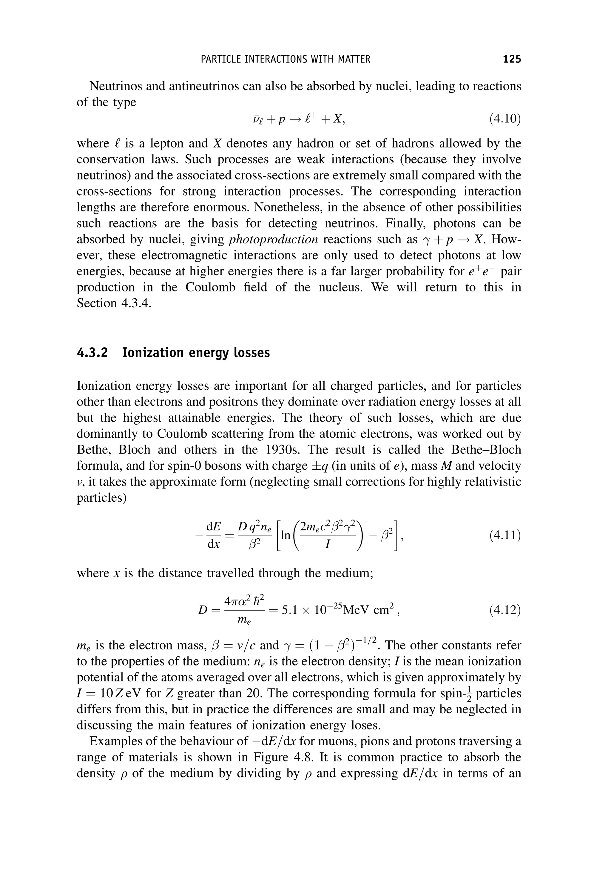
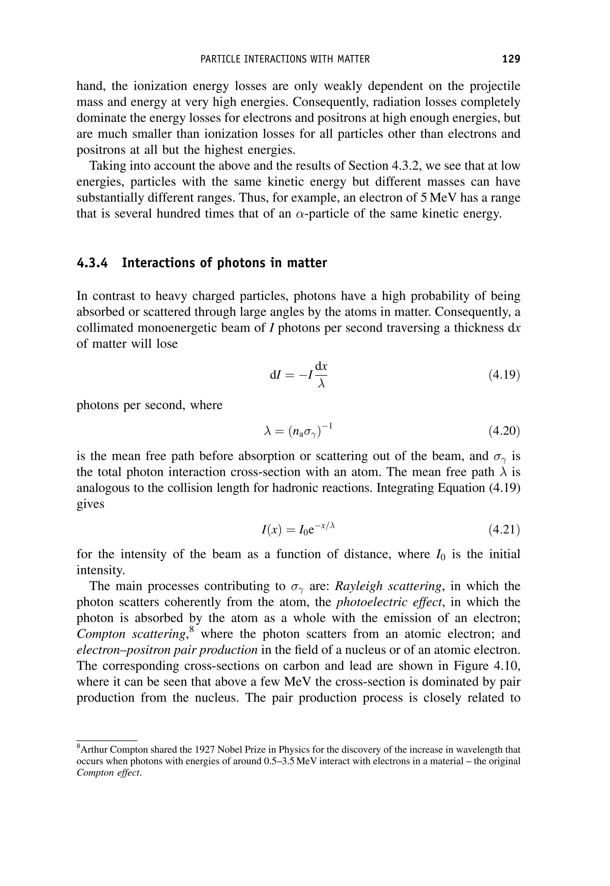

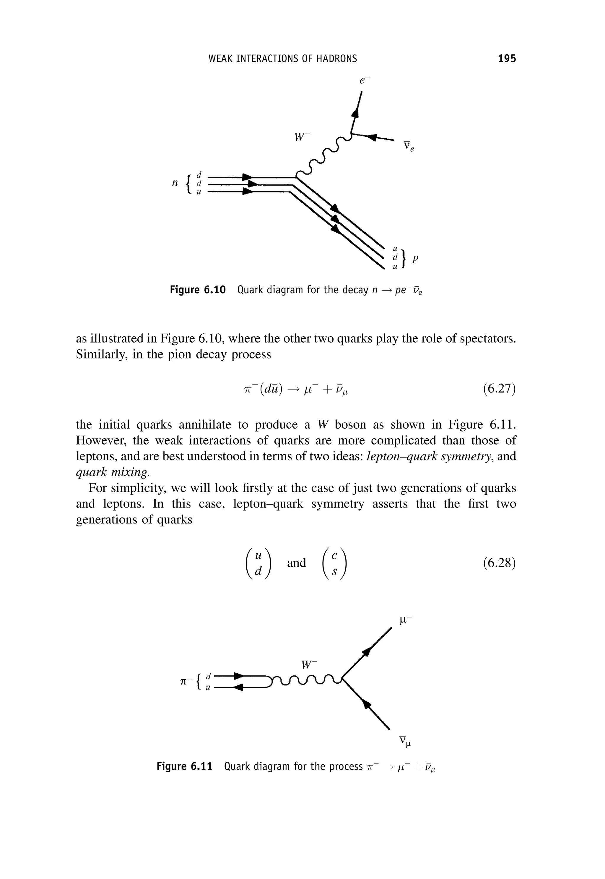
![both cases the total spin component along the z-axis is zero. This result is true for
all angles and the scattering is isotropic.
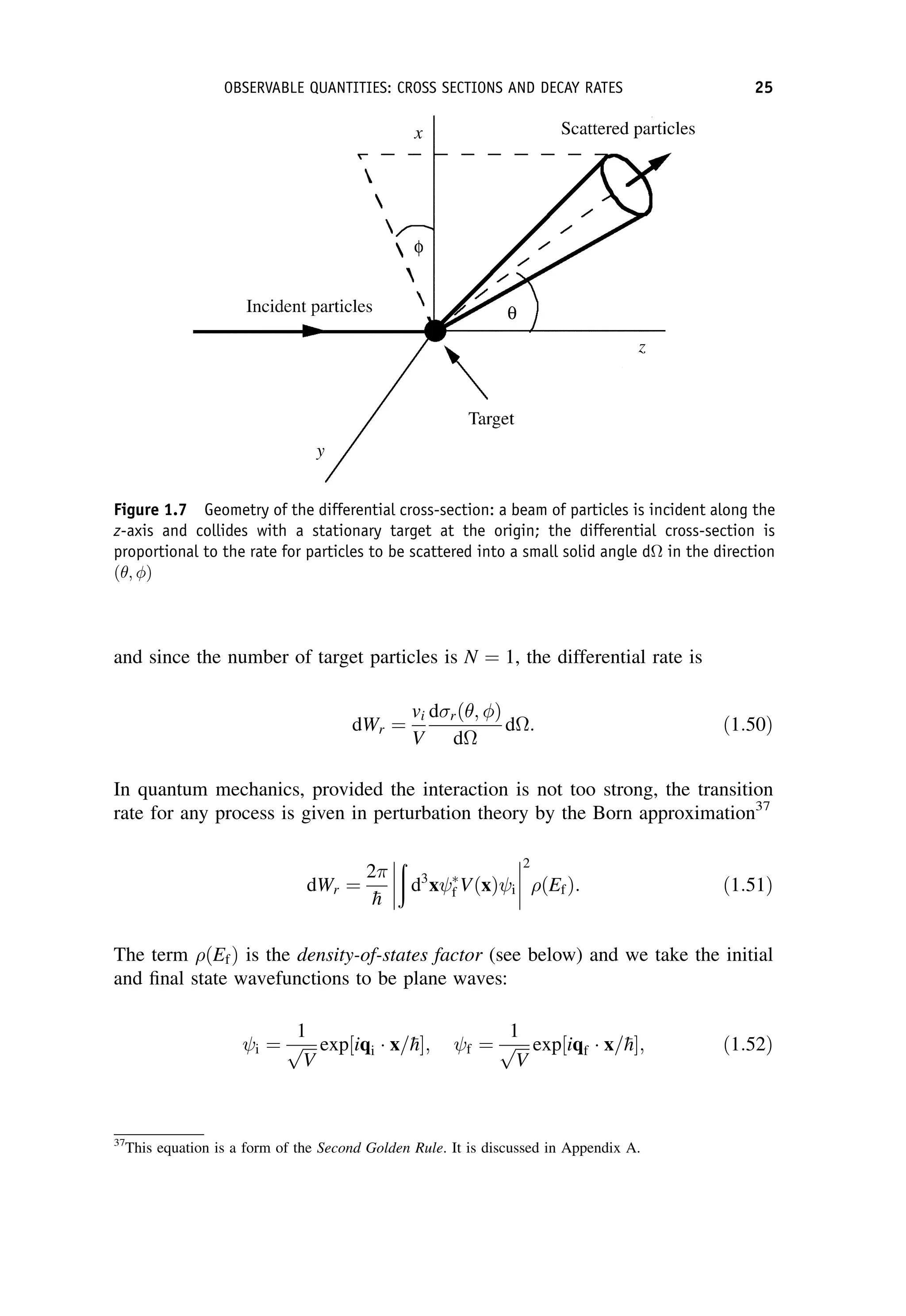
From this we can calculate the differential cross-section using the formulae of
Chapter 1. We will assume that the squared momentum transfer Q2
is such that
Q2
max M2
W c2
, so that the matrix element may be written [cf. Equation (6.1)]
fðe þ e
! e þ e
Þ ¼ GF; ð6:35Þ
where GF is the Fermi coupling constant of Equation (1.42), i.e.
GF ¼
4ð
hcÞ3
W
ðMW c2Þ2
ð6:36Þ
and W ¼ g2
=4
hc is the equivalent of the fine structure constant for charged
current weak interactions. Hence, using Equation (1.57) and recalling that the
velocities of both the neutrino and electron are equal to c,
d
d
ðee
Þ ¼
1
42
G2
F
ð
hcÞ4
E2
CM: ð6:37Þ
At high energies E2
CM is given by
E2
CM 2mec2
E; ð6:38Þ
where E is the energy of the neutrino. So finally the total cross-section is
totðee
Þ ¼
2mec2
G2
F
ð
hcÞ4
E ð6:39Þ
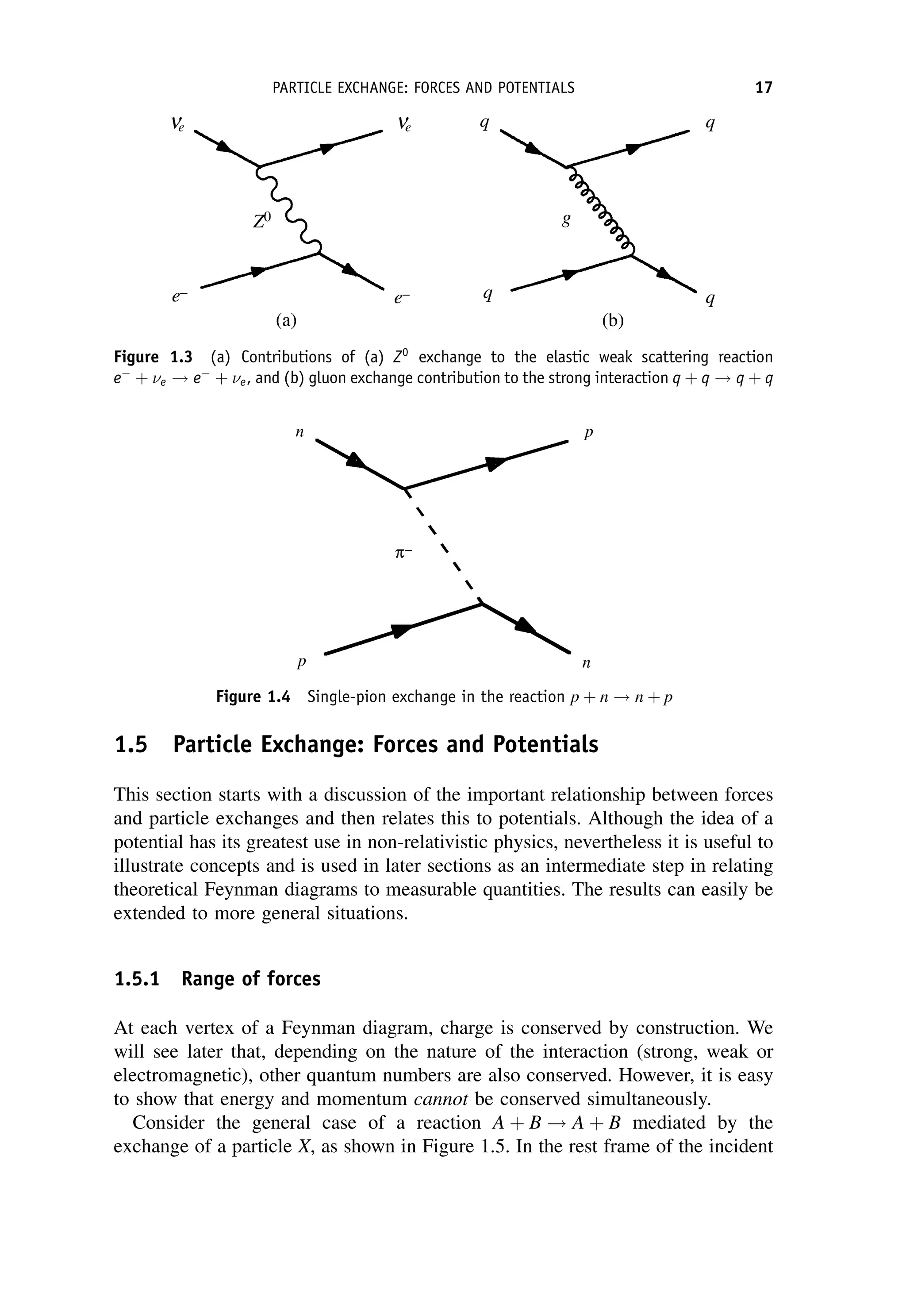
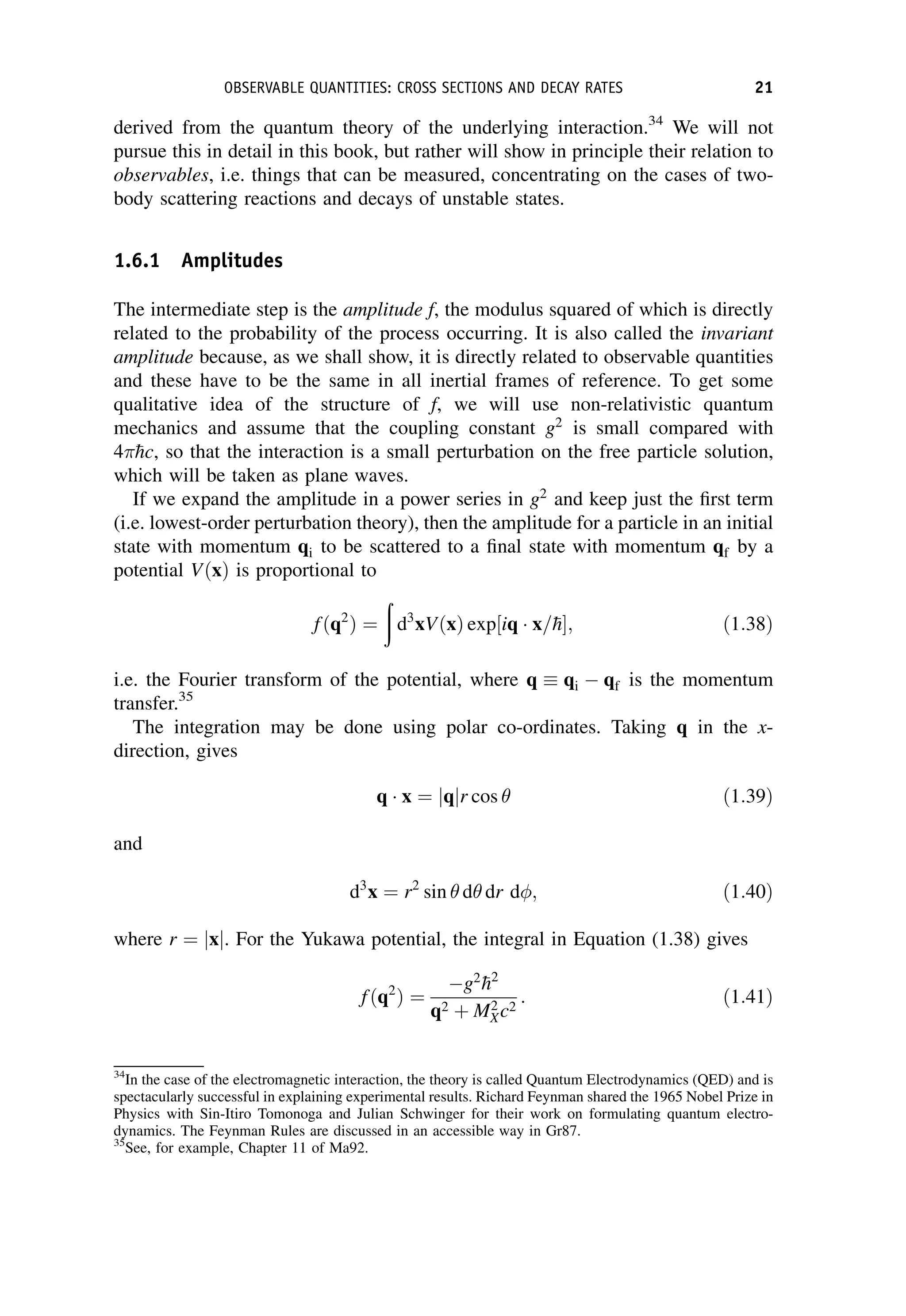
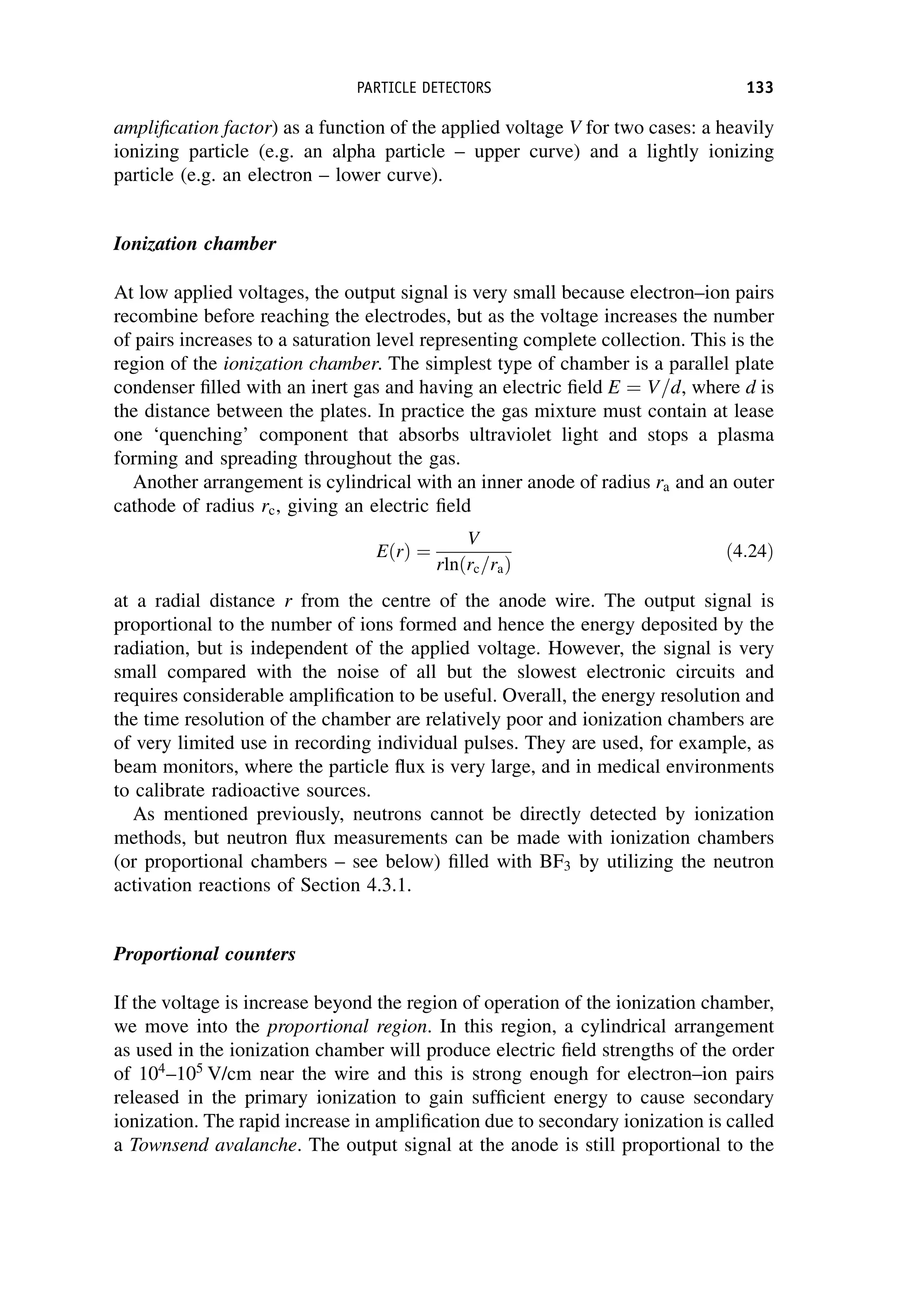
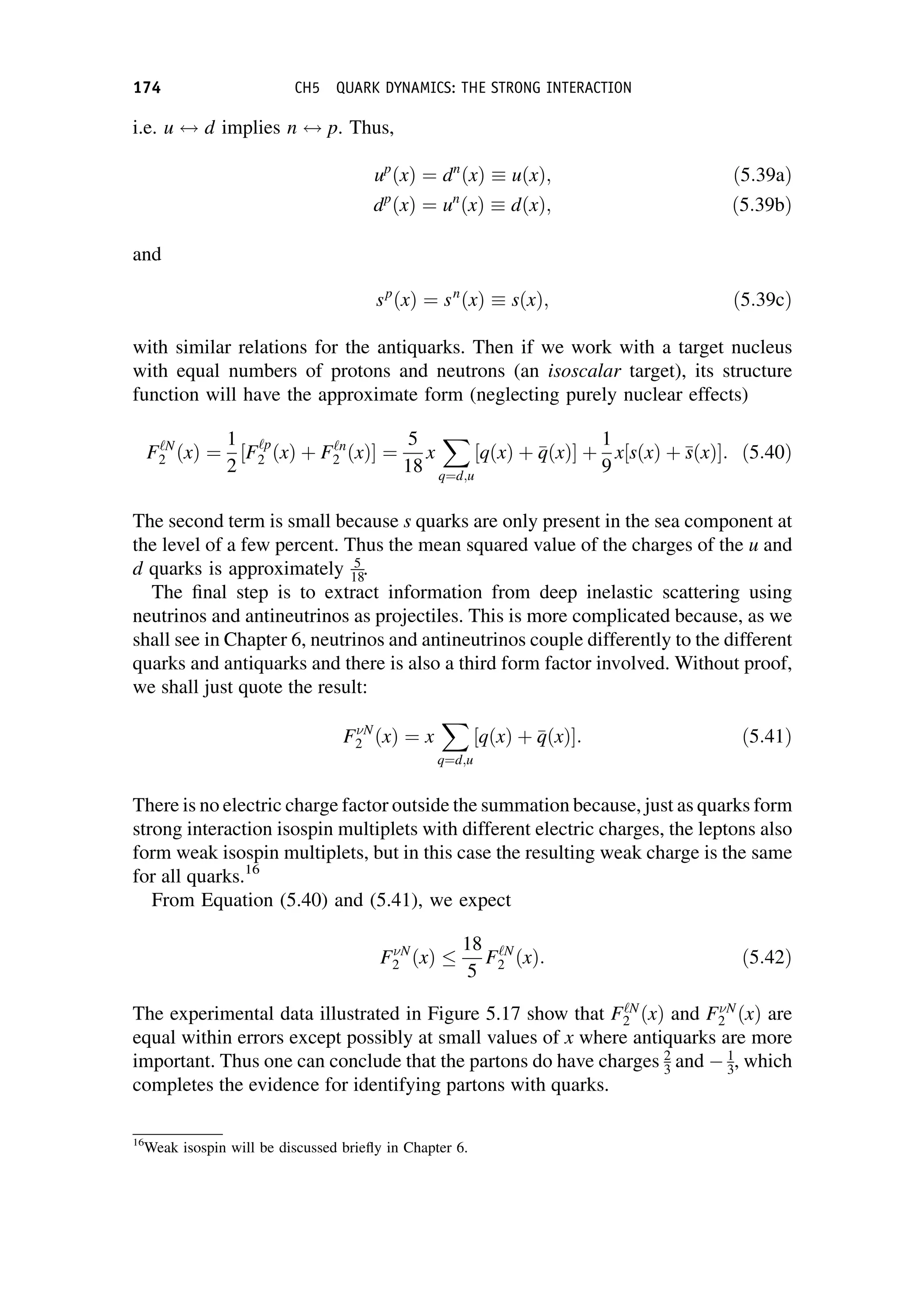
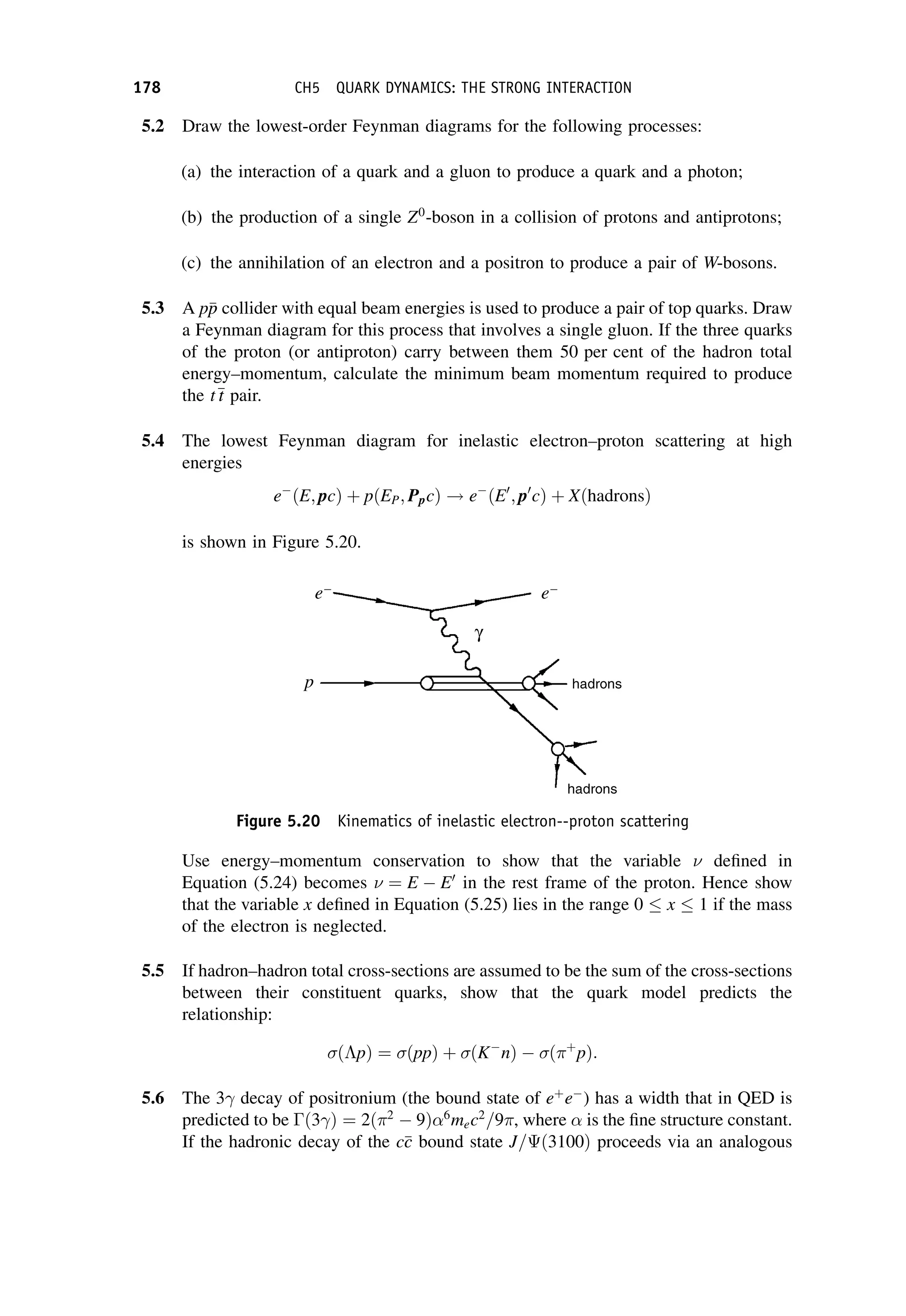
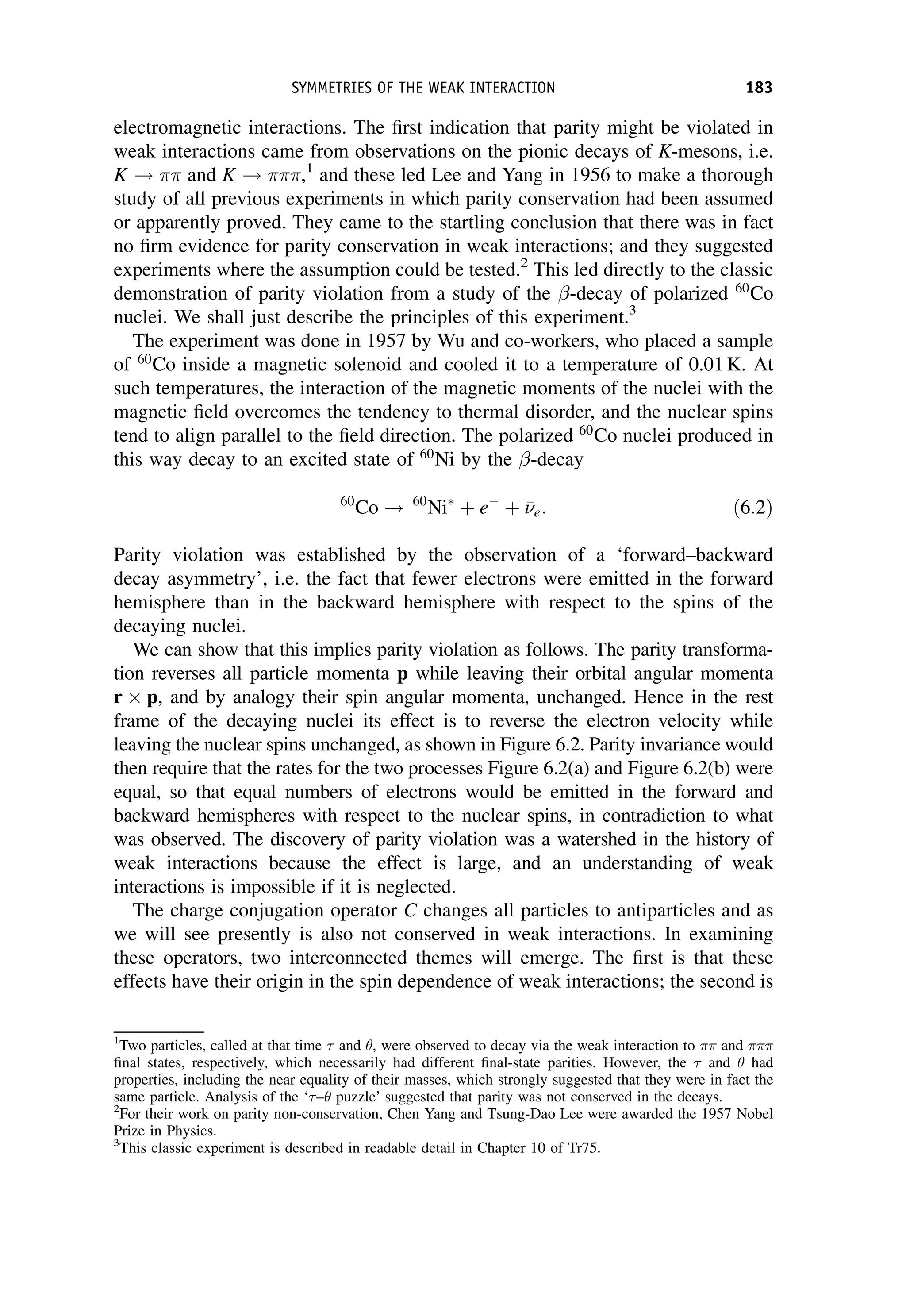
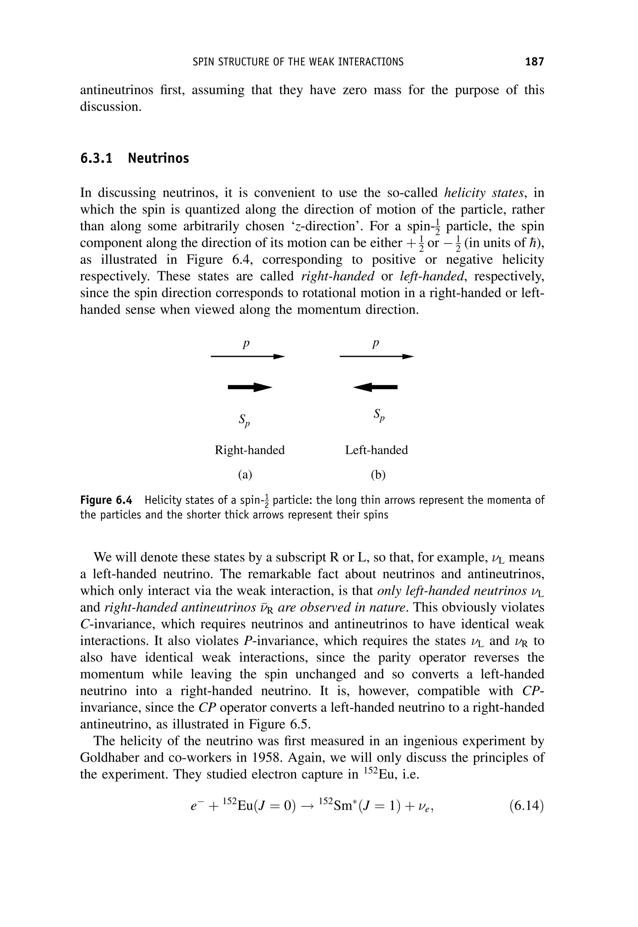
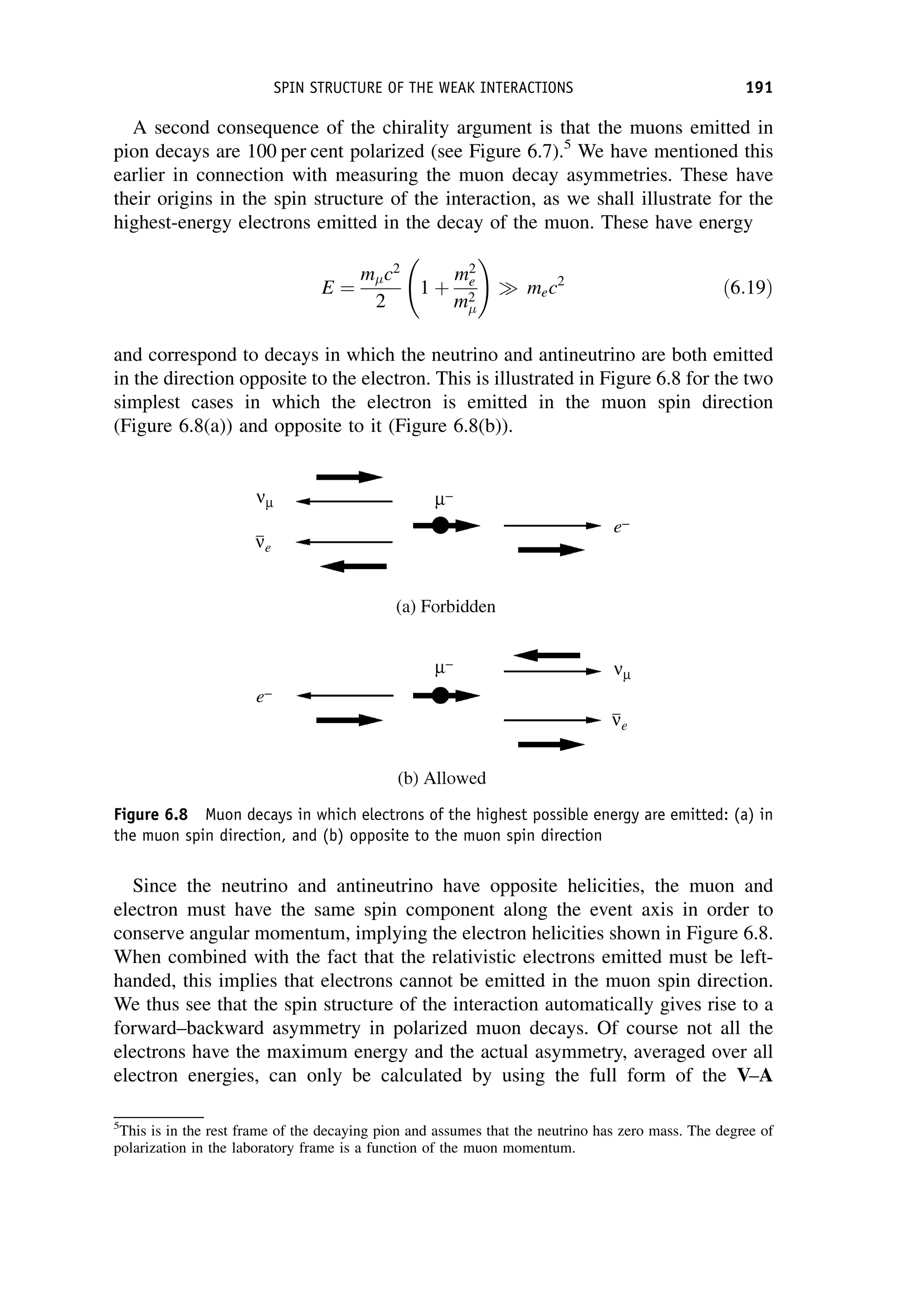
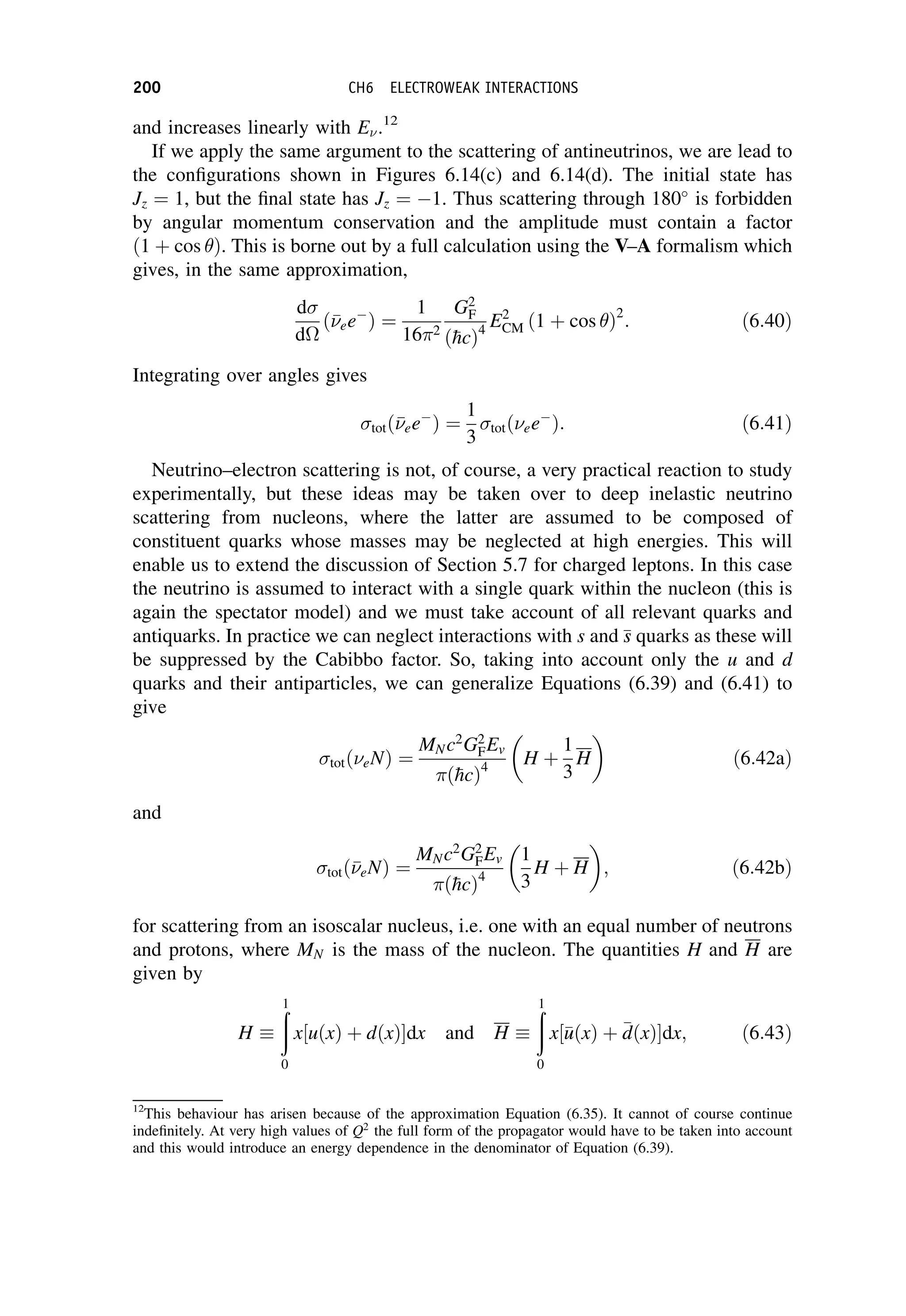
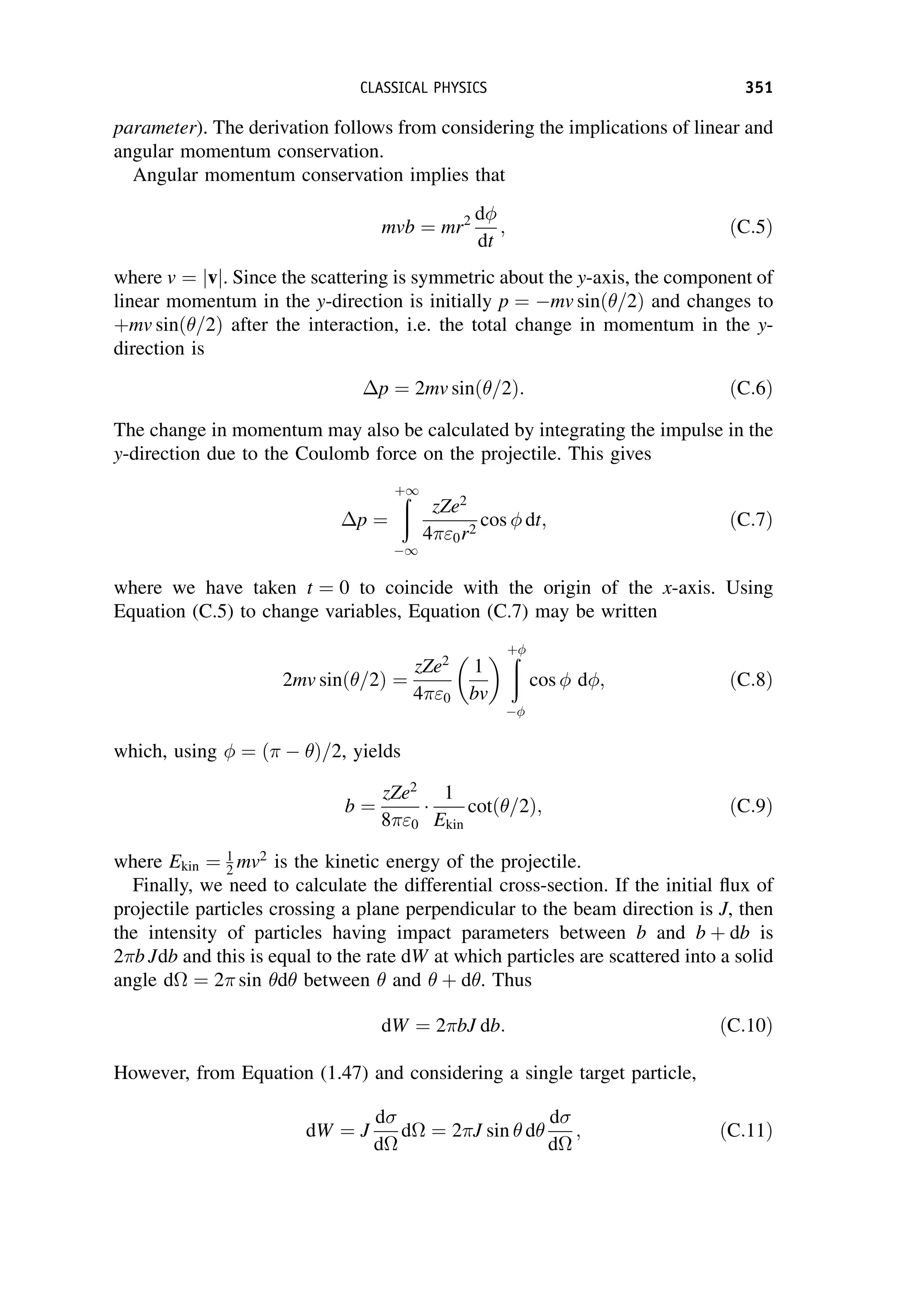
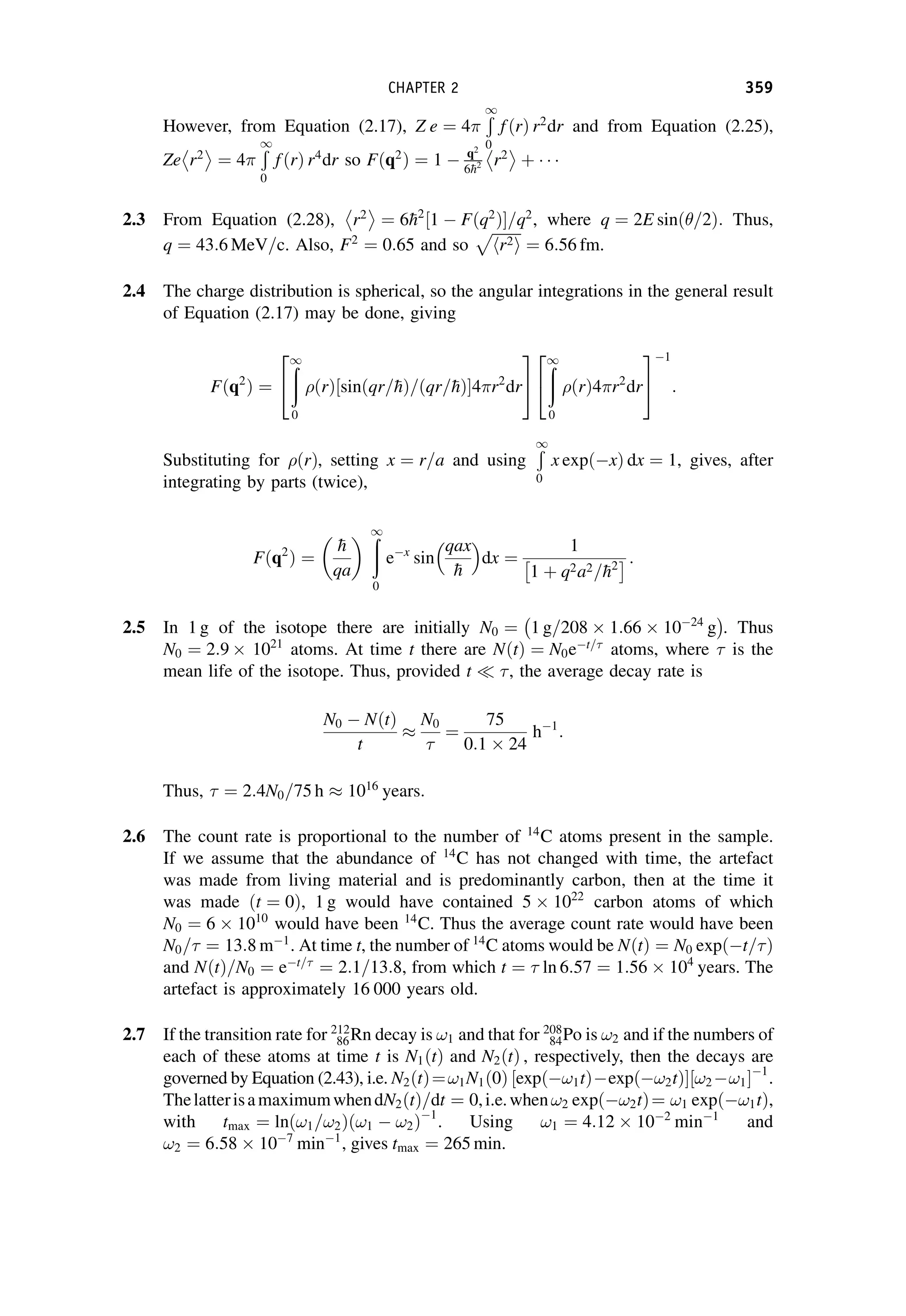
Figure 6.14 Spin (thick arrows) and momentum (thin arrows) configurations for ee
and
ee
interactions: (a) ee
before collision; (b) ee
after scattering through 180
; (c)
ee
before
collision; (d)
ee
after scattering through 180
WEAK INTERACTIONS OF HADRONS 199](https://image.slidesharecdn.com/martin-nuclearandparticlephysics-anintroduction-230216180050-11911371/75/Martin-Nuclear-and-Particle-Physics-An-Introduction-pdf-209-2048.jpg)
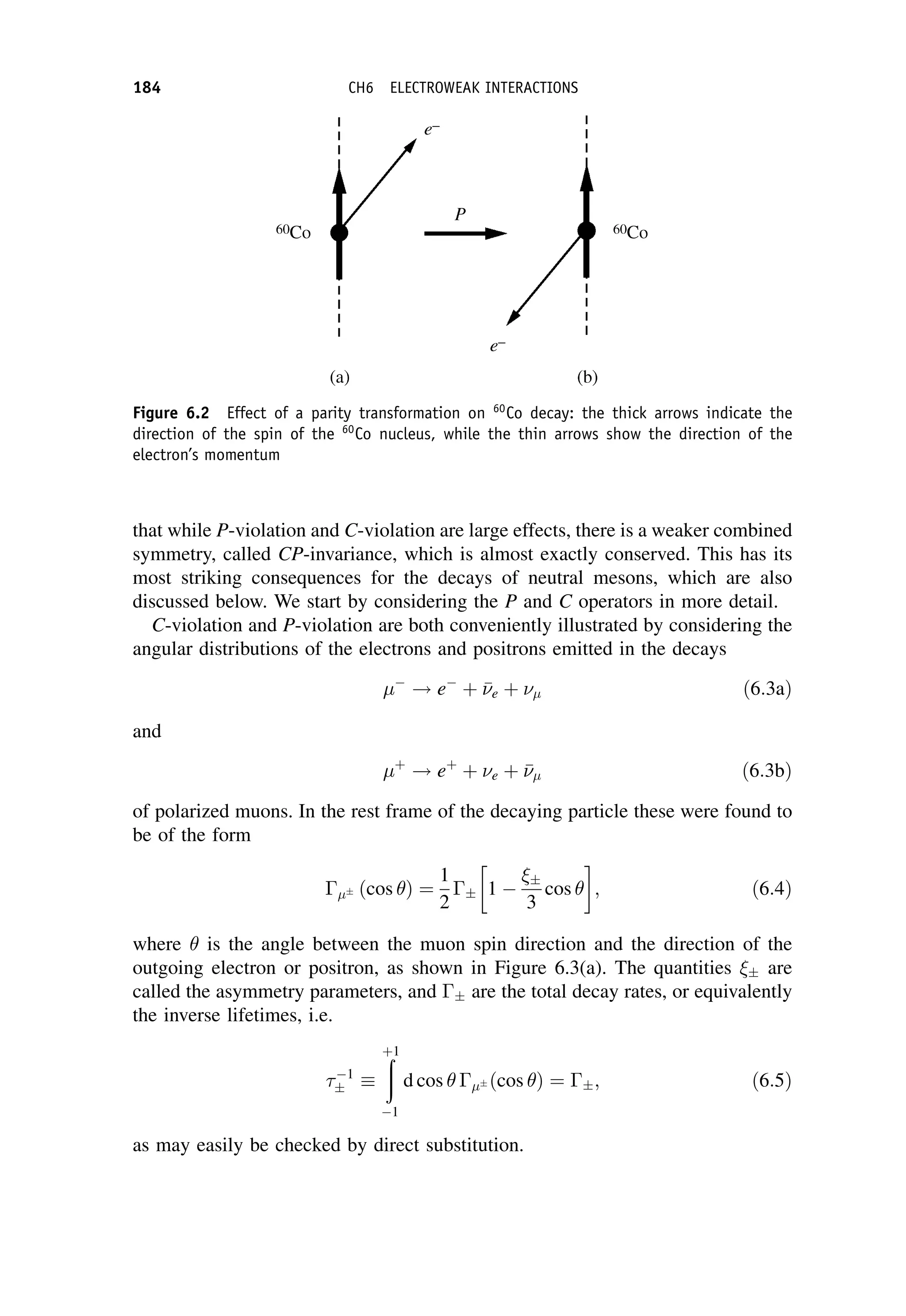
![so that
CPjK0
; 0i ¼ jK
0
; 0i; CPjK
0
; 0i ¼ jK0
; 0i: ð6:48Þ
Thus CP eigenstates K0
1;2 are
jK0
1;2; 0i ¼
1
ffiffiffi
2
p jK0
; 0i jK
0
; j0i
n o
ðCP ¼ 1Þ: ð6:49Þ
If CP is conserved, then K0
1 should decay entirely to states with CP ¼ 1 and K0
2
should decay entirely into states with CP ¼ 1. We examine the consequences of
this for decays leading to pions in the final state.
Consider the state 0
0
. Since the kaon has spin-0, by angular momentum
conservation the pion pair must have zero orbital angular momentum in the rest
frame of the decaying particle. Its parity is therefore given by [cf. Equation (1.14)]
P ¼ P2
1
ð ÞL
¼ 1; ð6:50Þ
where P ¼ 1 is the intrinsic parity of the pion. The C-parity is given by
C ¼ ðC0 Þ2
¼ 1; ð6:51Þ
where C0 ¼ 1 is the C-parity of the neutral pion. Combining these results gives
CP ¼ 1. The same result holds for the þ
final state.
The argument for three-pion final states þ
0
and 0
0
0
is more compli-
cated, because there are two orbital angular momenta to consider, If we denote by
L12 the orbital angular momentum of one pair (either þ
or 0
0
) in their
mutual centre-of-mass frame, and L3 is the orbital angular momentum of the third
pion about the centre-of-mass of the pair in the overall centre-of-mass frame, then
the total orbital angular momentum L L12 þ L3 ¼ 0, since the decaying particle
has spin-0. This can only be satisfied if L12 ¼ L3. This implies that the parity of the
final state is
P ¼ P3
1
ð ÞL12
1
ð ÞL3
¼ 1: ð6:52Þ
For the 0
0
0
final state, the C-parity is
C ¼ C0
ð Þ3
¼ 1 ð6:53Þ
and combining these results gives CP ¼ 1 overall. The same result can be shown
to hold for the þ
0
final state.
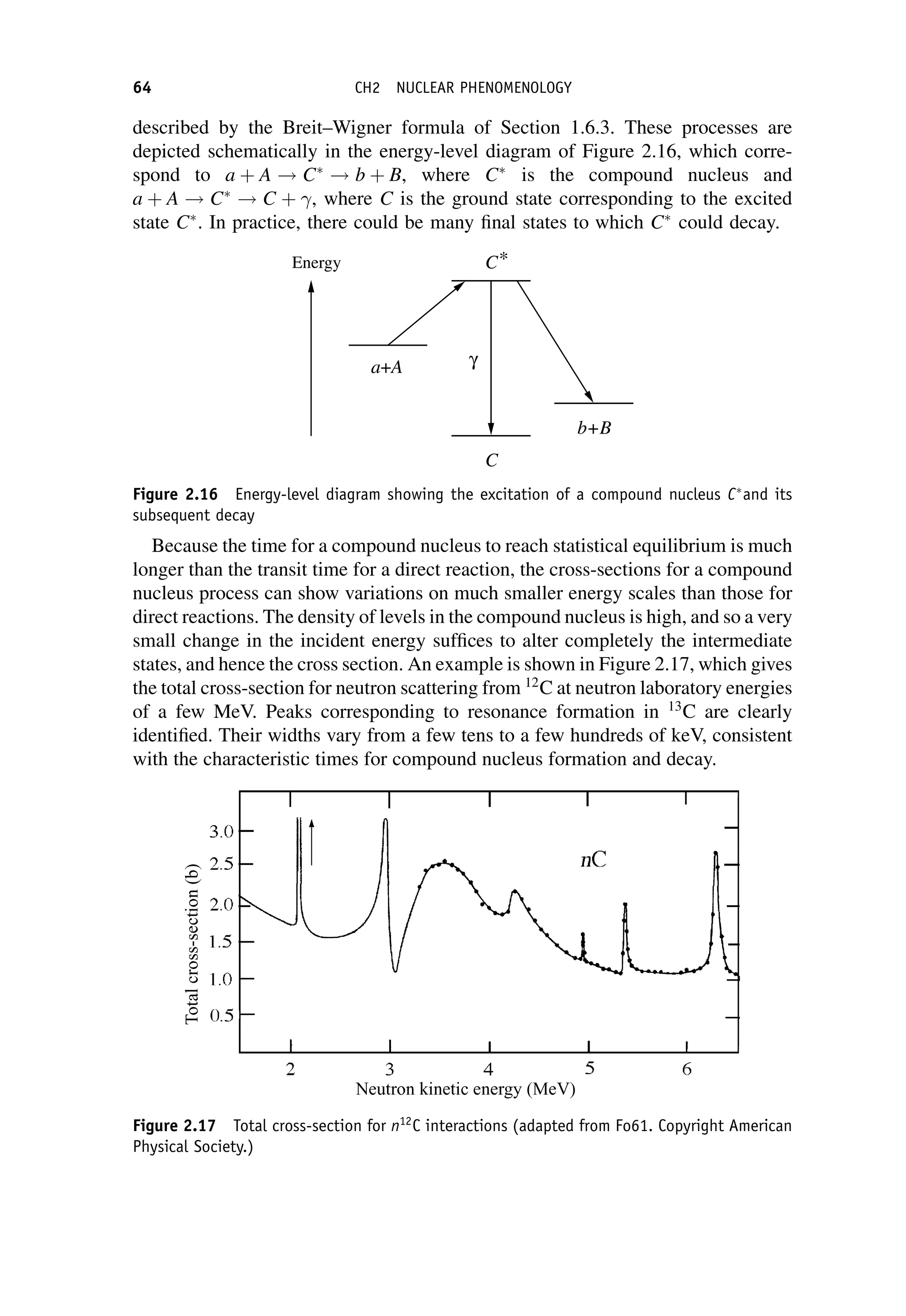
The experimental position is that two neutral kaons are observed, called K0
-short
and K0
-long, denoted K0
S and K0
L, respectively. They have almost equal masses of
about 499 MeV/c2
, but very different lifetimes and decay modes. The K0
S has a
NEUTRAL MESON DECAYS 203](https://image.slidesharecdn.com/martin-nuclearandparticlephysics-anintroduction-230216180050-11911371/75/Martin-Nuclear-and-Particle-Physics-An-Introduction-pdf-213-2048.jpg)

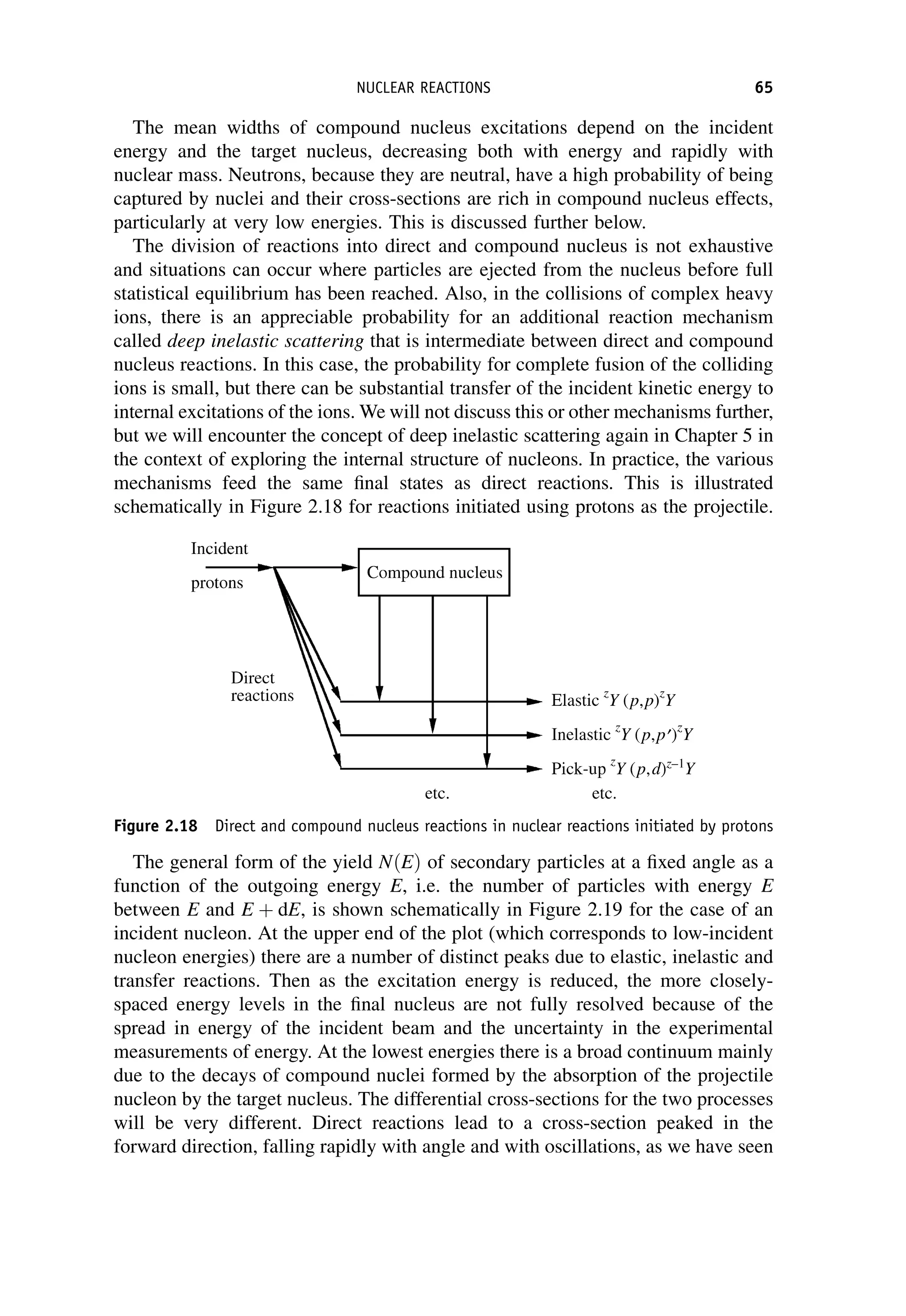
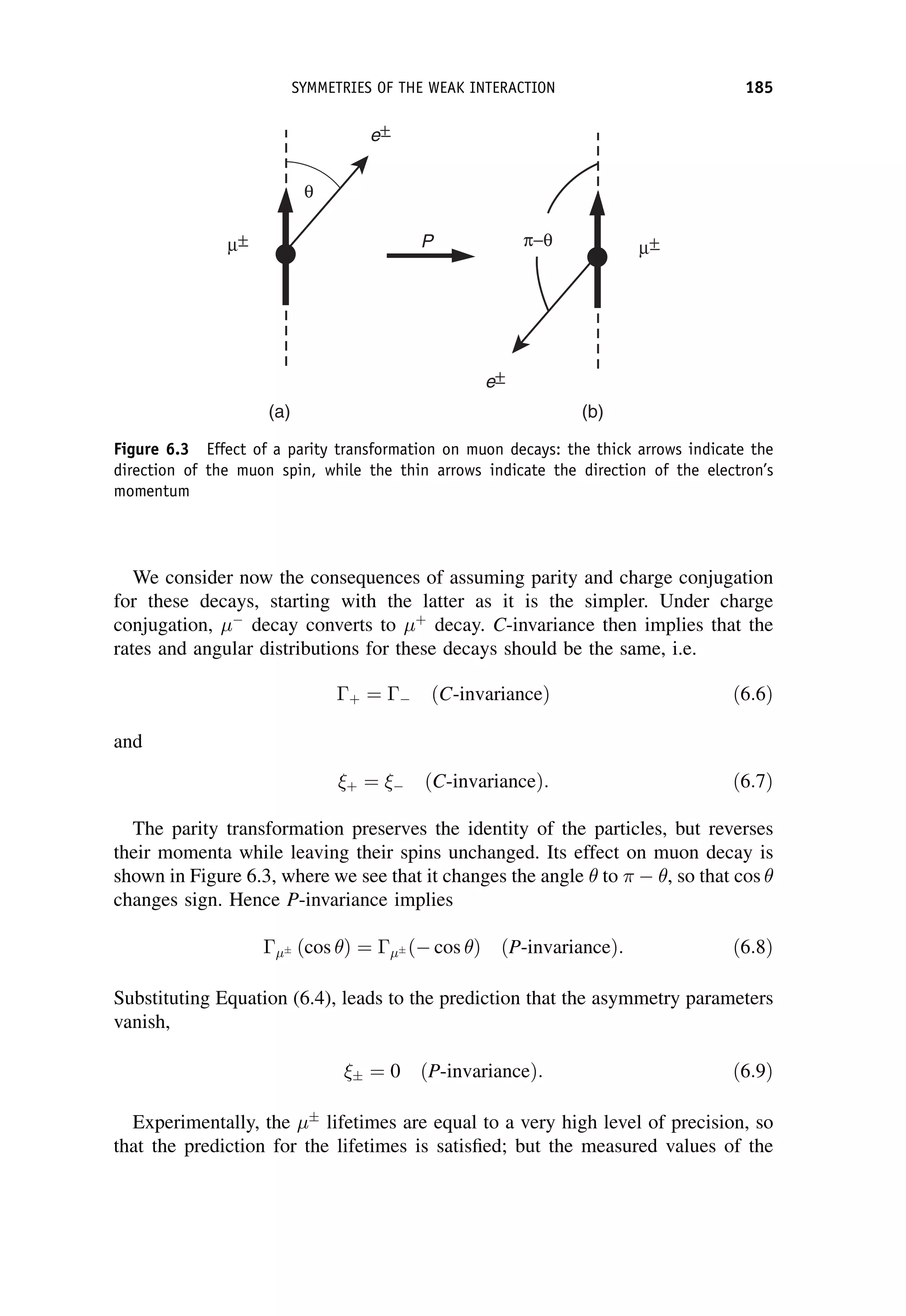
![The matrix element can in general be written in terms of five basic Lorentz
invariant interaction operators, ^
O
O:
Mfi ¼
ð
f ðg^
O
OÞi d3
x; ð7:58Þ
where f and i are total wavefunctions for the final and initial states, respectively,
g is a dimensionless coupling constant, and the integral is over three-dimensional
space The five categories are called scalar (S), pseudo-scalar (P), vector (V), axial-
vector (A), and tensor (T ); the names having their origin in the mathematical
transformation properties of the operators. (We have met the V and A forms
previously in Chapter 6 on the electroweak interaction.) The main difference
between them is the effect on the spin states of the parent and daughter nuclei.
When there are no spins involved, and at low energies, ðg^
O
OÞ is simply the interaction
potential, i.e. that part of the potential that is responsible for the change of state of the
system.
Fermi guessed that ^
O
O would be of the vector type, since electromagnetism is a
vector interaction, i.e. it is transmitted by a spin-1 particle – the photon. (Decays of
the vector type are called Fermi transitions.) We have seen from the work of
Chapter 6 that we now know that the weak interaction violates parity conservation
and is correctly written as a mixture of both vector and axial-vector interactions (the
latter are called Gamow–Teller transitions in nuclear physics), but as long as we are
not concerned with the spins of the nuclei, this does not make much difference, and
we can think of the matrix element in terms of a classical weak interaction potential,
like the Yukawa potential. Applying a bit of modern insight, we can assume the
potential is of extremely short range (because of the large mass of the W boson), in
which case we have seen that we can approximate the interaction by a point-like
form and the matrix element then becomes simply a constant, which we write as
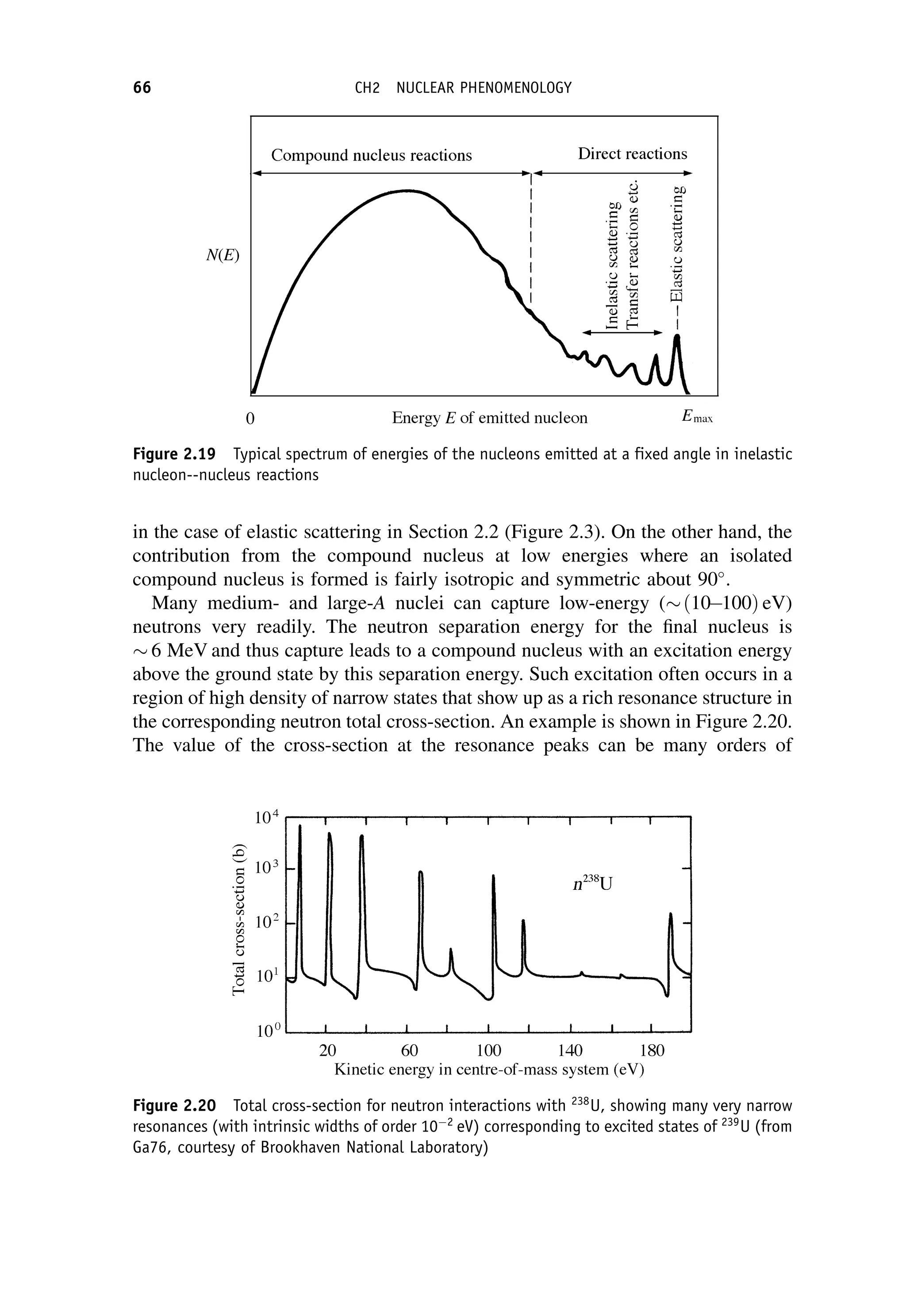
Mfi ¼
GF
V
; ð7:59Þ
where GF is the Fermi coupling constant we met in Chapter 6. It has dimensions
[energy][length]3
and is related to the charged current weak interaction coupling
W by
GF ¼
4ð
hcÞ3
W
ðMW c2Þ2
: ð7:60Þ
In Equation (7.59) it is convenient to factor out an arbitrary volume V, which is used
to normalize the wavefunctions. (It will eventually cancel out with a factor in the
density-of-states term.)
In nuclear theory, the Fermi coupling constant GF is taken to be a universal
constant and with appropriate corrections for changes of the nuclear state this
b-DECAY 243](https://image.slidesharecdn.com/martin-nuclearandparticlephysics-anintroduction-230216180050-11911371/75/Martin-Nuclear-and-Particle-Physics-An-Introduction-pdf-253-2048.jpg)
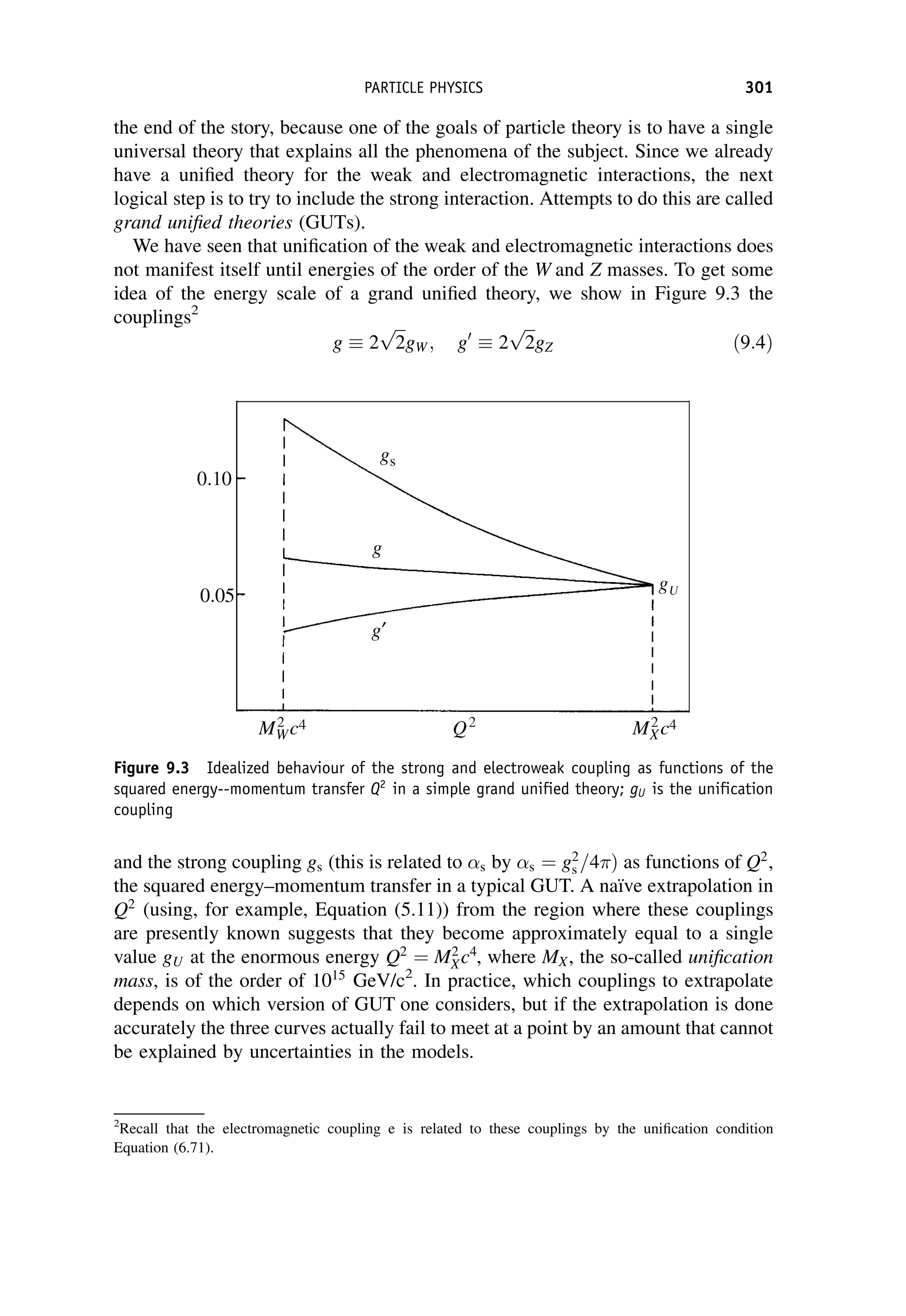
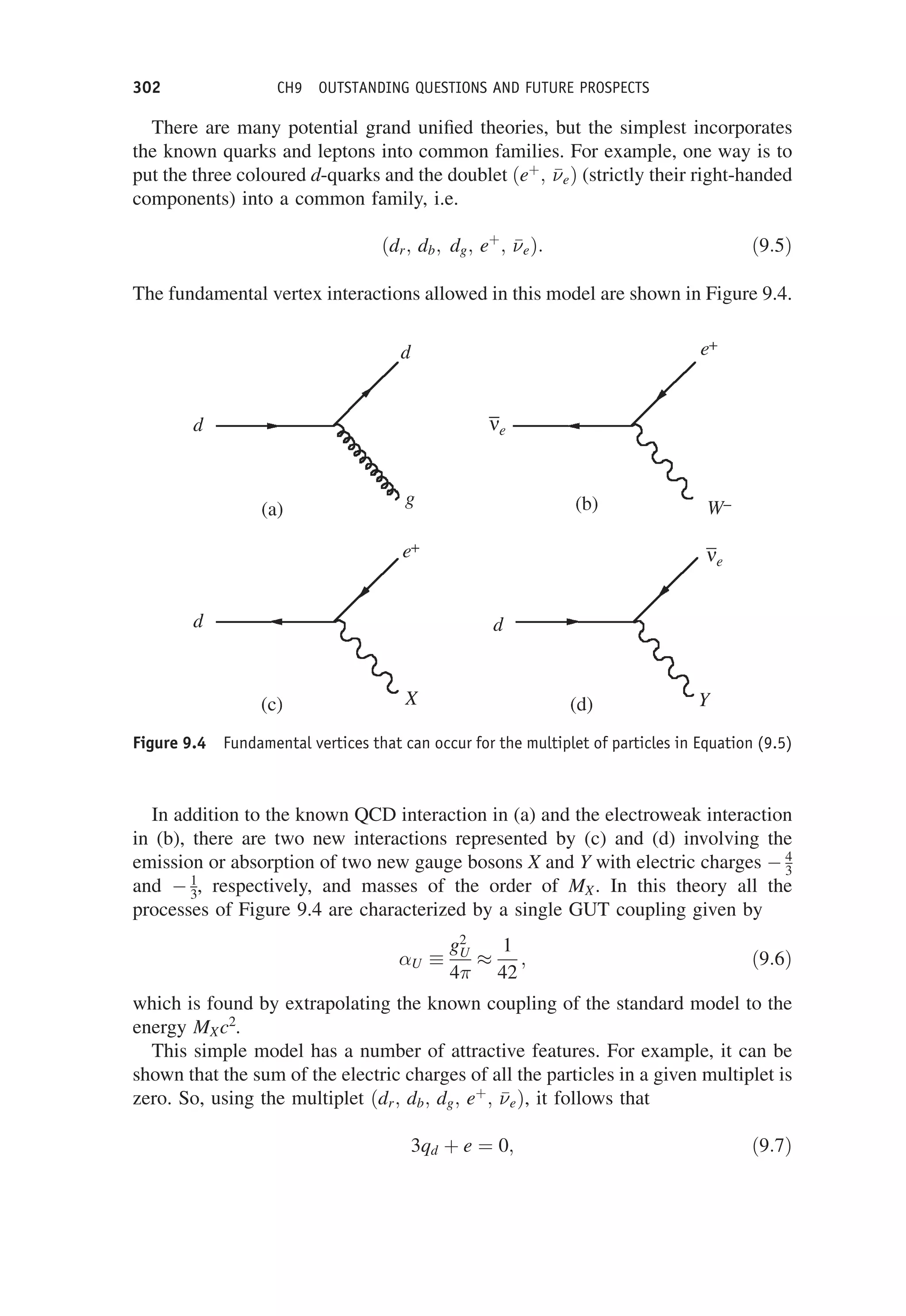
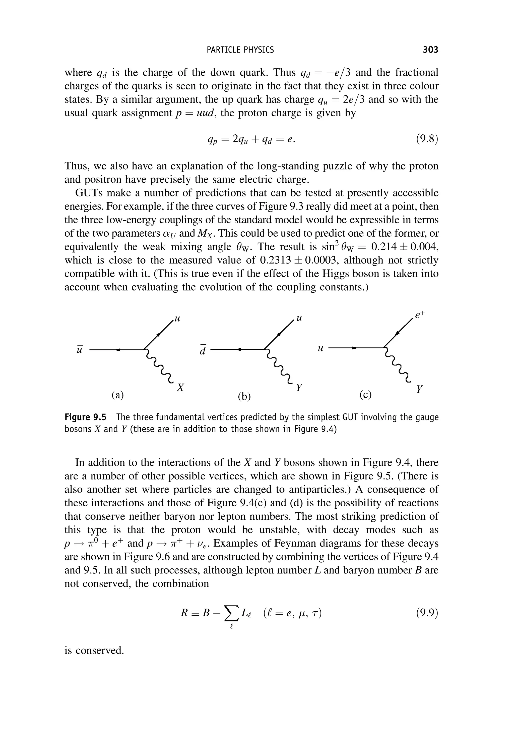
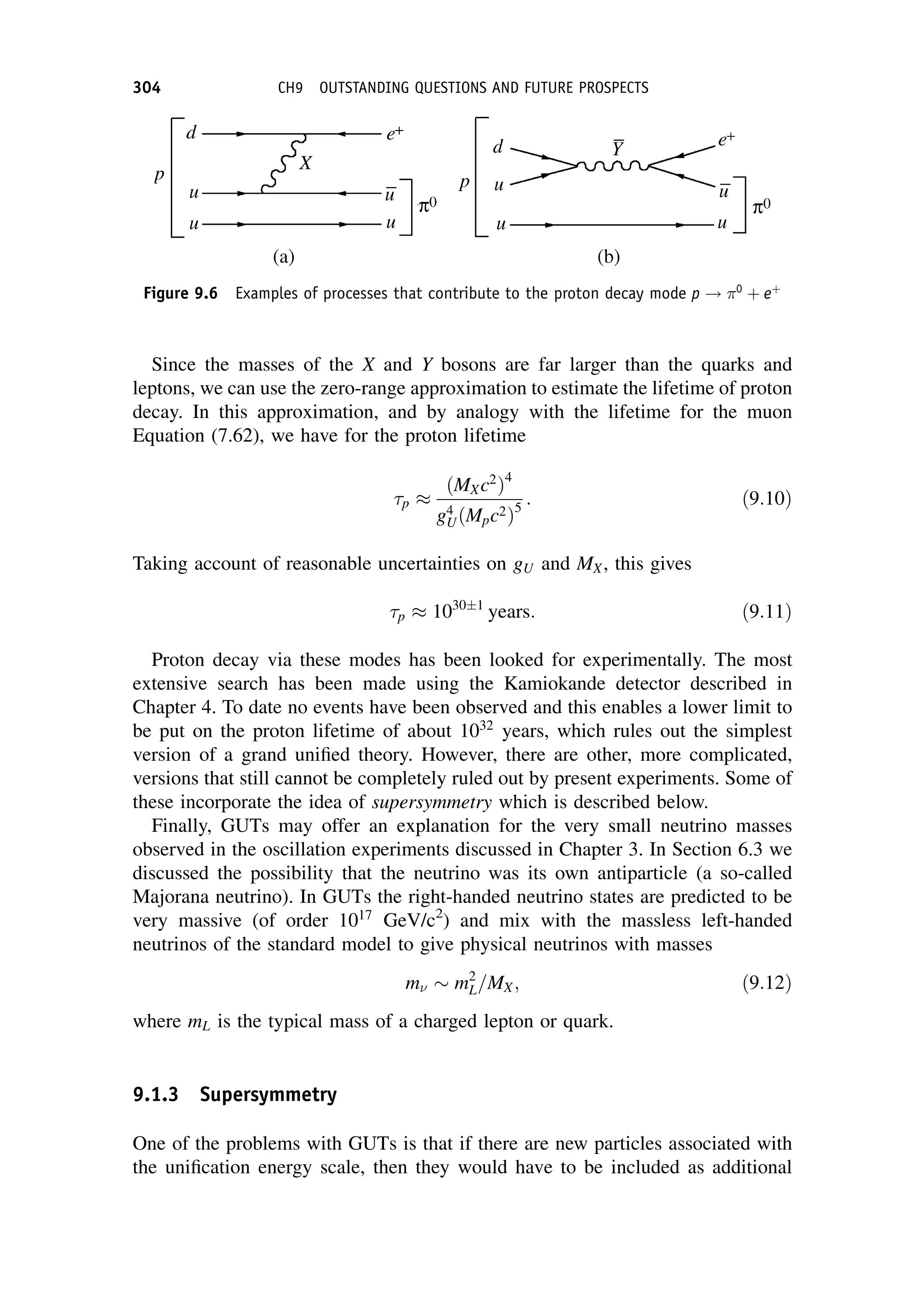

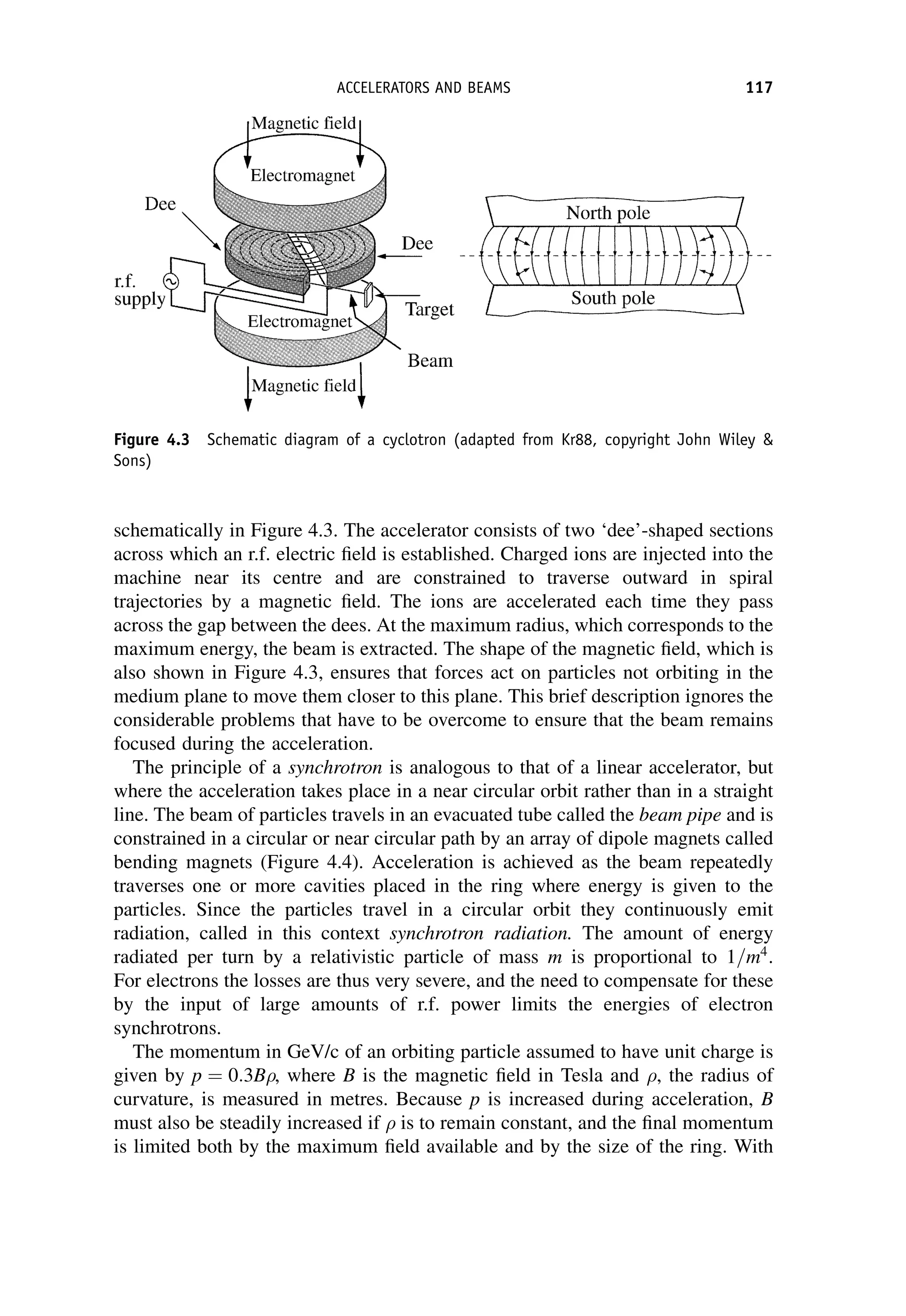
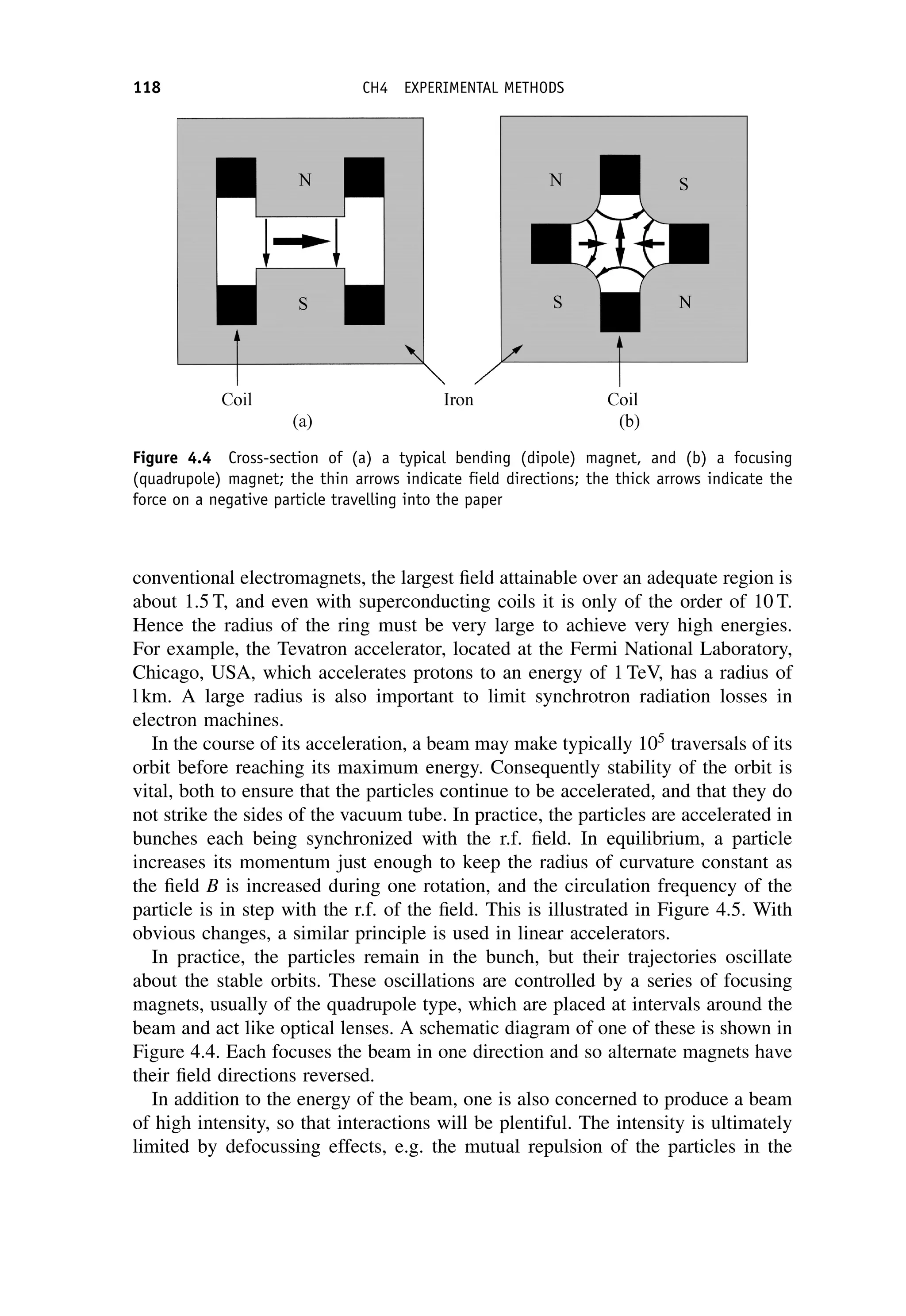
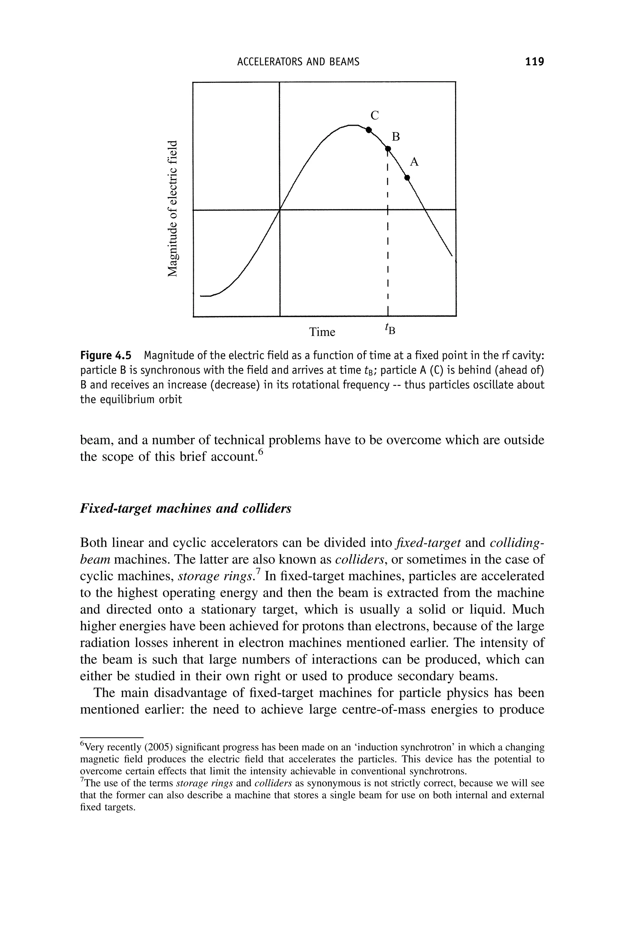
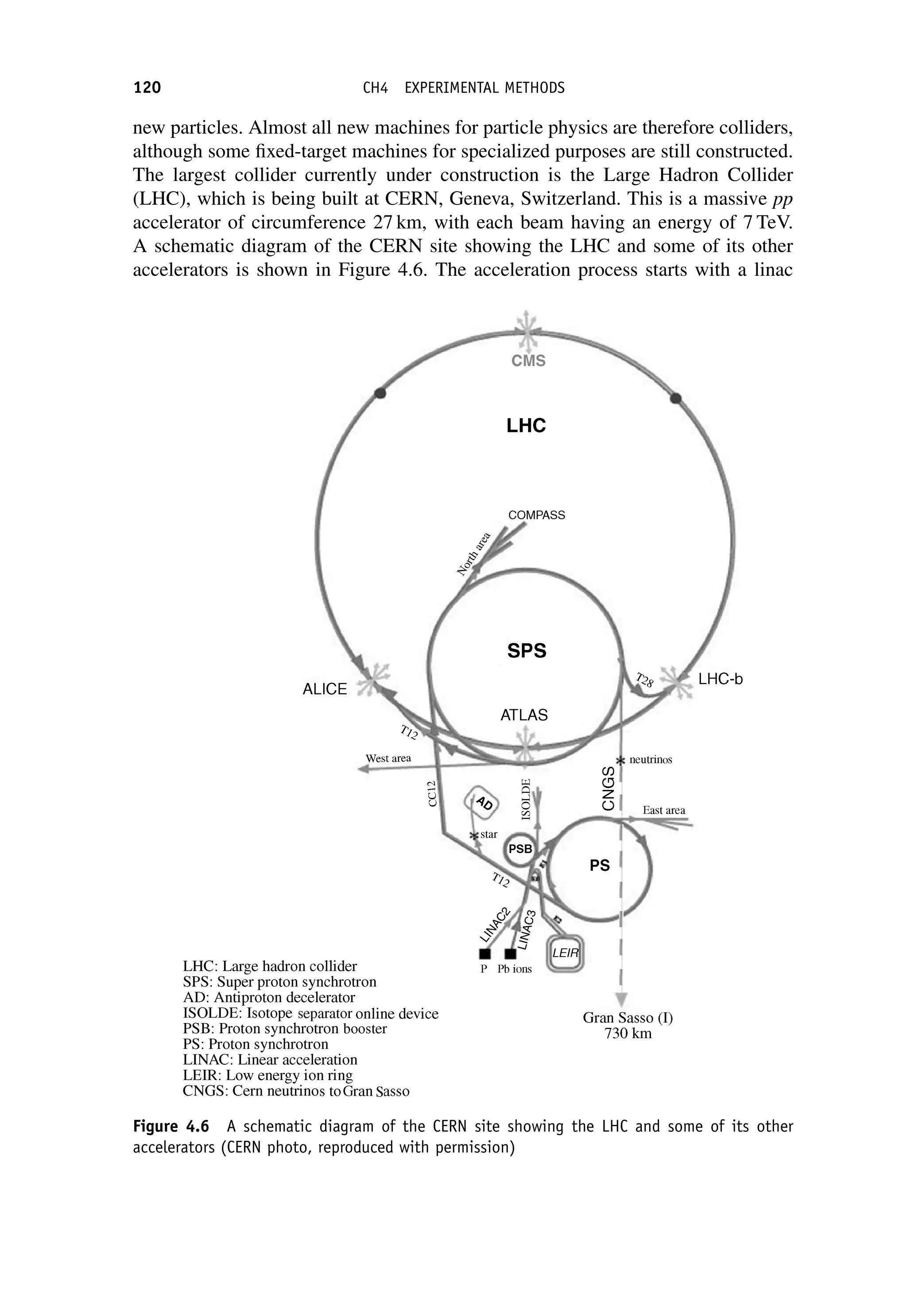
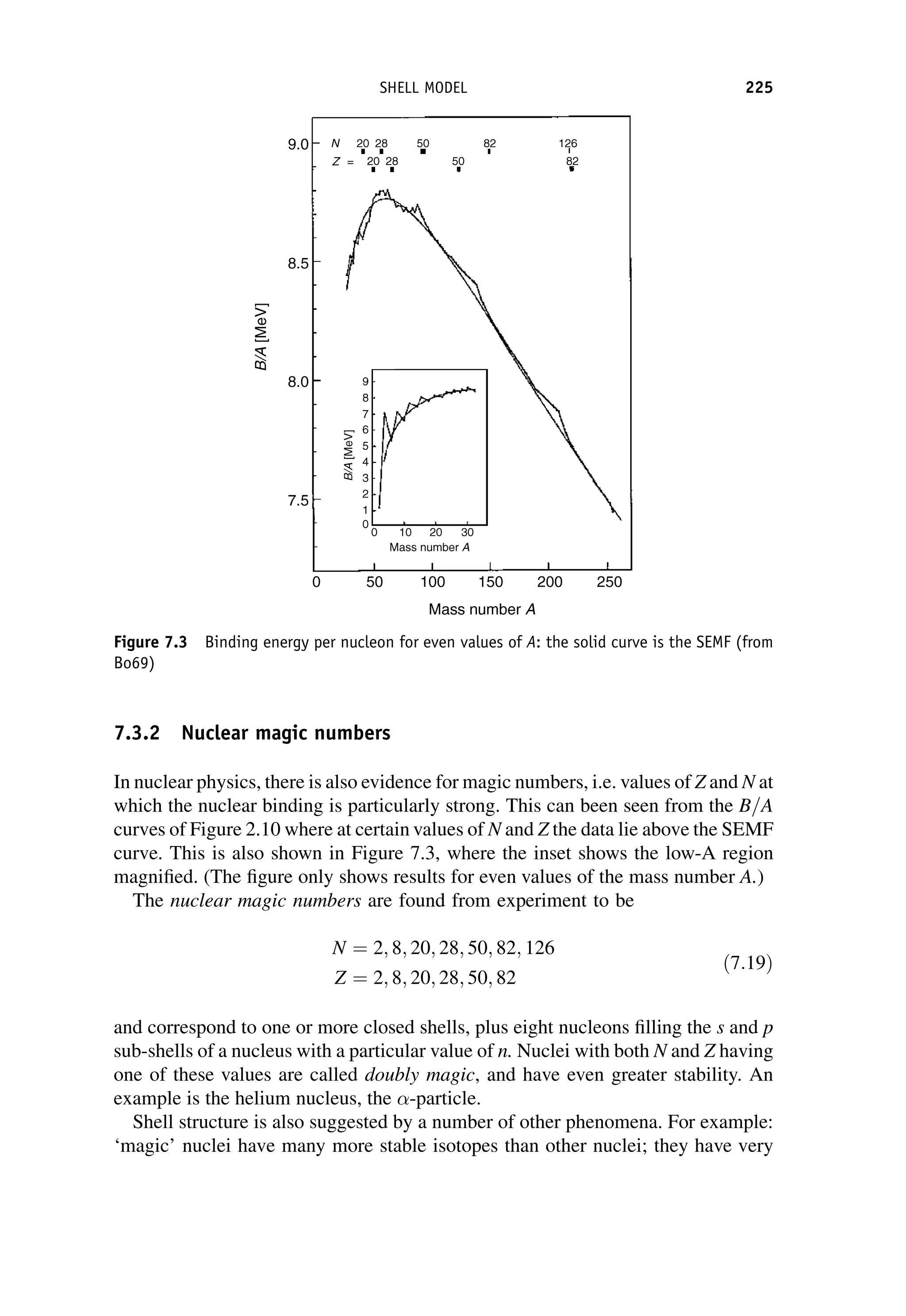
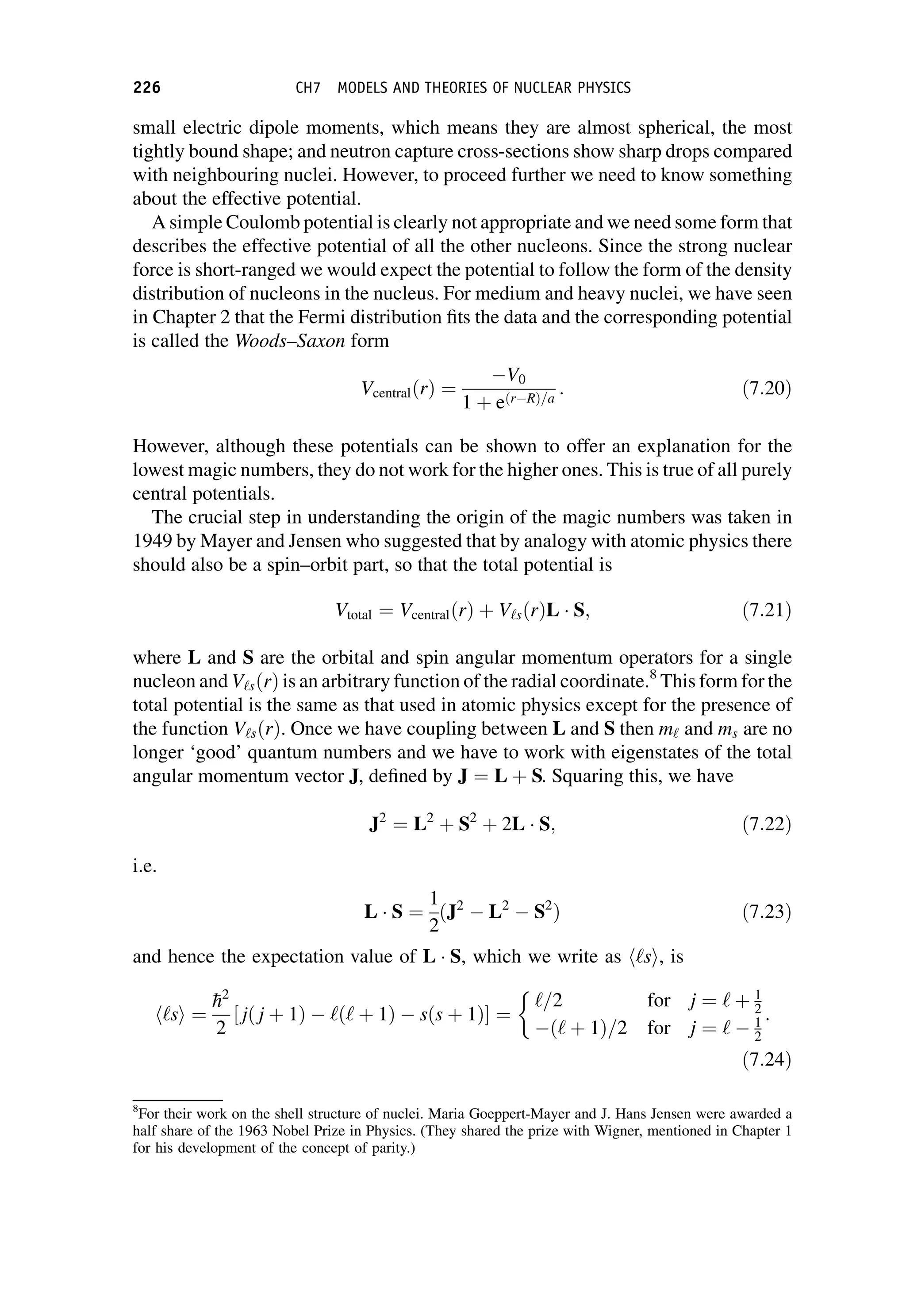
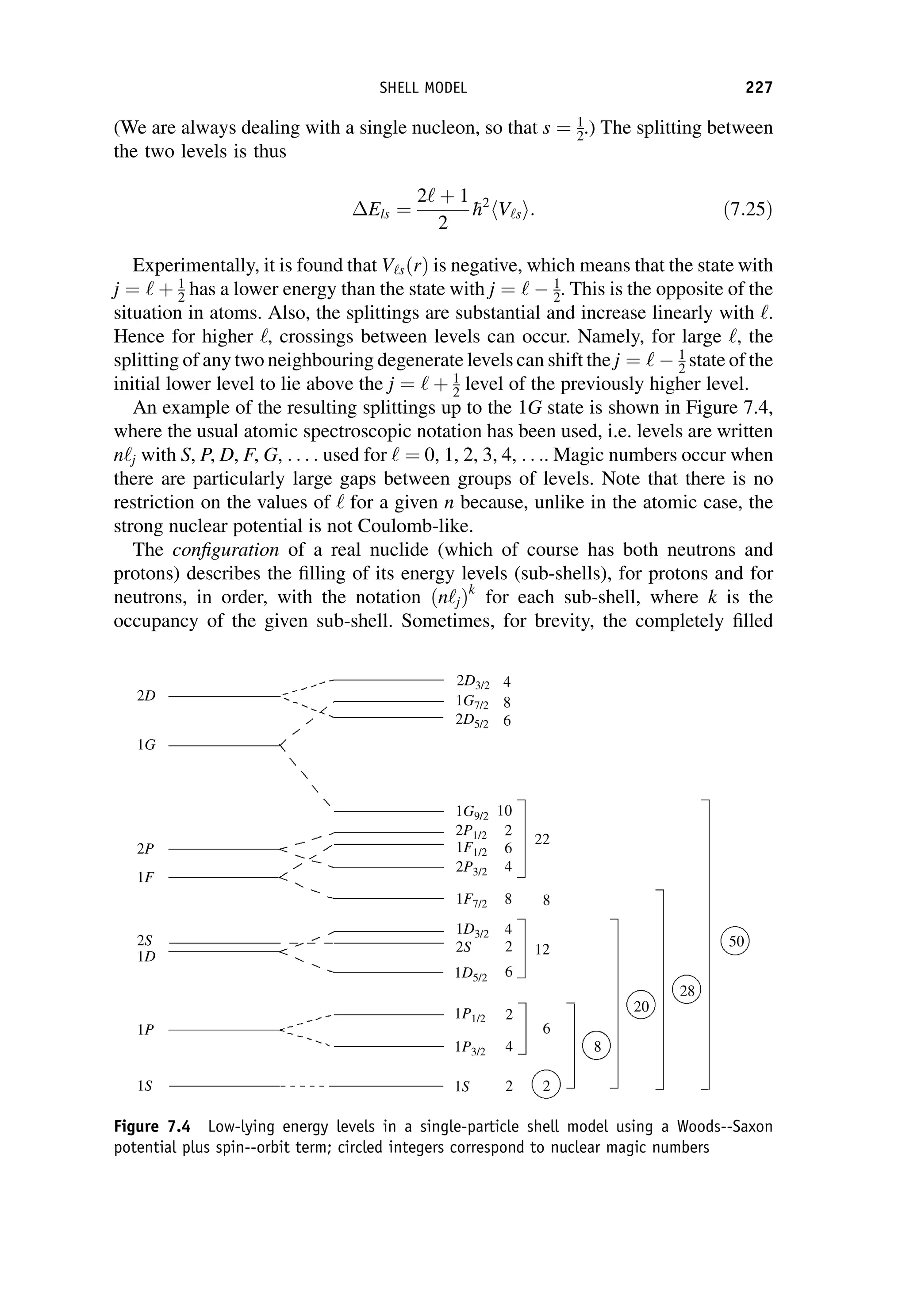
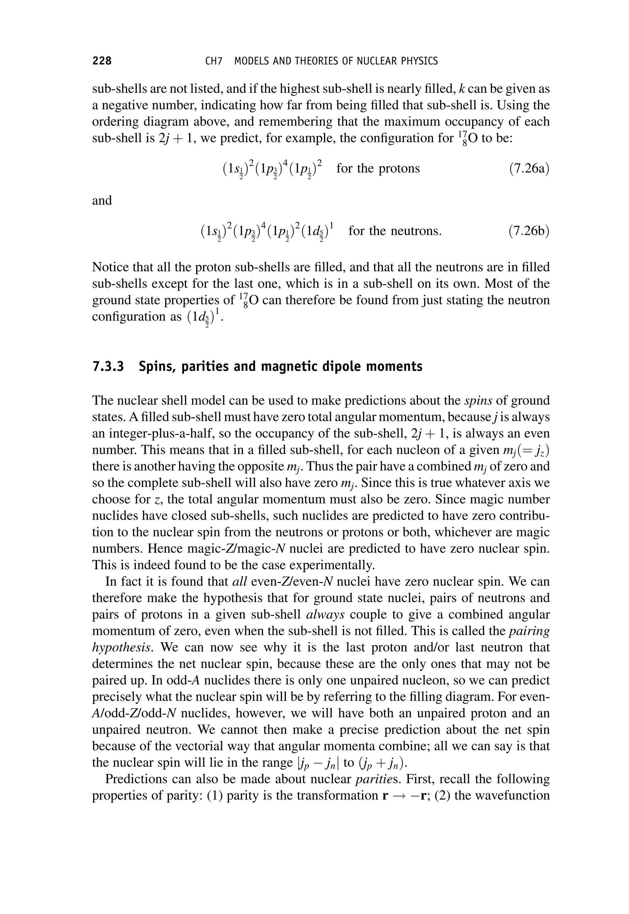
This document provides an overview of the textbook "Nuclear and Particle Physics" by B. R. Martin, which covers topics in nuclear and particle physics for an introductory course. The textbook is published by John Wiley & Sons and is intended to give students an overview of the key concepts and discoveries in nuclear and particle physics rather than rigorous proofs. It covers subjects such as the history and basic concepts of nuclear and particle physics, nuclear and particle phenomenology, experimental methods, models of the strong and electroweak interactions, applications of nuclear physics, and outstanding questions.


