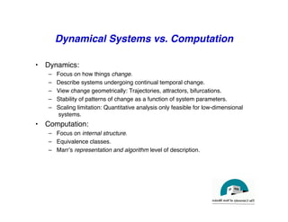
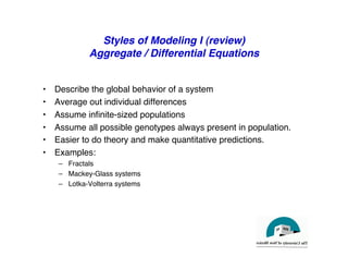
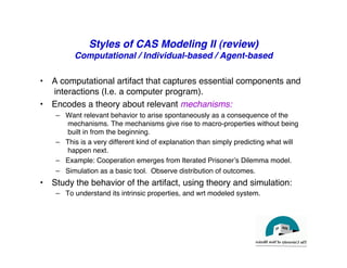
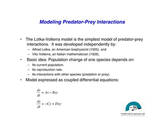
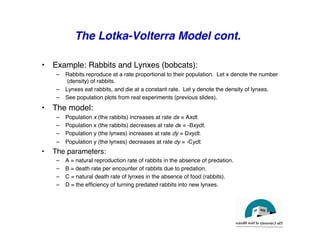
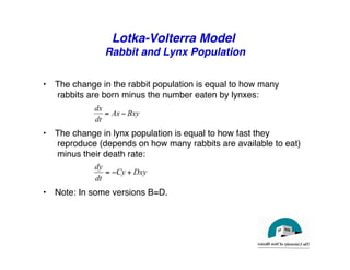
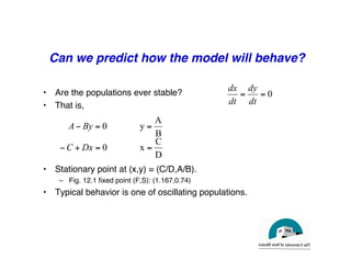
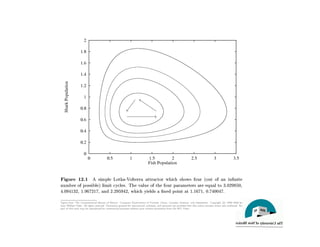
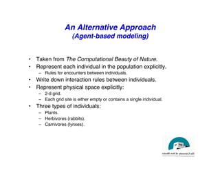
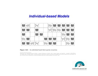
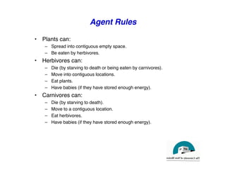
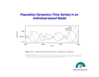
This document discusses predator-prey models including the classic Lotka-Volterra model and alternative agent-based models. The Lotka-Volterra model uses differential equations to model species populations over time, assuming homogeneous mixing and infinite population sizes. An agent-based model represents each individual explicitly on a grid and uses rules for local interactions, allowing for heterogeneity, finite populations, and spatial effects not captured by Lotka-Volterra. Both approaches can generate oscillating population dynamics resembling real predator-prey data, but the agent-based model provides a more individual-level perspective.

1. Predator-Prey Models
Stephanie Forrest
Dept. of Computer Science
Univ. of New Mexico
Albuquerque, NM
http://cs.unm.edu/~forrest
forrest@cs.unm.edu

2. Dynamical Systems vs. Computation
"
• Dynamics:"
– Focus on how things change.!
– Describe systems undergoing continual temporal change."
– View change geometrically: Trajectories, attractors, bifurcations."
– Stability of patterns of change as a function of system parameters."
– Scaling limitation: Quantitative analysis only feasible for low-dimensional
systems."
• Computation:"
– Focus on internal structure.!
– Equivalence classes."
– Marrʼs representation and algorithm level of description."

3. Styles of Modeling I (review)
Aggregate / Differential Equations
"
• Describe the global behavior of a system"
• Average out individual differences"
• Assume infinite-sized populations"
• Assume all possible genotypes always present in population."
• Easier to do theory and make quantitative predictions."
• Examples:"
– Fractals"
– Mackey-Glass systems"
– Lotka-Volterra systems"

4. Styles of CAS Modeling II (review)
Computational / Individual-based / Agent-based
"
• A computational artifact that captures essential components and
interactions (I.e. a computer program)."
• Encodes a theory about relevant mechanisms:!
– Want relevant behavior to arise spontaneously as a consequence of the
mechanisms. The mechanisms give rise to macro-properties without being
built in from the beginning."
– This is a very different kind of explanation than simply predicting what will
happen next."
– Example: Cooperation emerges from Iterated Prisonerʼs Dilemma model."
– Simulation as a basic tool. Observe distribution of outcomes."
• Study the behavior of the artifact, using theory and simulation:"
– To understand its intrinsic properties, and wrt modeled system."

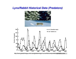
5. Lynx Historical Data (Predators)
"
[D'Ancona, 1954]"

6. Lynx/Rabbit Historical Data (Predators)
"
http://www.globalchange.umich.edu/globalchange1/current/lectures/predation/predation.html
"

7. Paramecium Data
"

8. Predator-Prey Dynamics in Demand Destruction and Oil Prices
"
The predator-prey oscillations of price increases and demand destruction/production increases
superimposed on top of a geological depletion scenario--note how the volatility fo the predator-prey
dynamic works to conceal the underlying geological and geopolitical trends. "

9. Modeling Predator-Prey Interactions
"
• The Lotka-Volterra model is the simplest model of predator-prey
interactions. It was developed independently by:"
– Alfred Lotka, an American biophysicist (1925), and"
– Vito Volterra, an Italian mathematician (1926)."
• Basic idea: Population change of one species depends on:"
– Its current population."
– Its reproduction rate."
– Its interactions with other species (predation or prey)."
• Model expressed as coupled differential equations:"
Bxy
Ax
dt
dx
−
=
Dxy
Cy
dt
dy
+
−
=

10. The Lotka-Volterra Model cont.
"
• Example: Rabbits and Lynxes (bobcats):"
– Rabbits reproduce at a rate proportional to their population. Let x denote the number
(density) of rabbits."
– Lynxes eat rabbits, and die at a constant rate. Let y denote the density of lynxes."
– See population plots from real experiments (previous slides)."
• The model:"
– Population x (the rabbits) increases at rate dx = Axdt.!
– Population x (the rabbits) decreases at rate dx = -Bxydt."
– Population y (the lynxes) increases at rate dy = Dxydt."
– Population y (the lynxes) decreases at rate dy = -Cydt."
• The parameters:"
– A = natural reproduction rate of rabbits in the absence of predation."
– B = death rate per encounter of rabbits due to predation."
– C = natural death rate of lynxes in the absence of food (rabbits)."
– D = the efficiency of turning predated rabbits into new lynxes."

11. Lotka-Volterra Model
Rabbit and Lynx Population
"
• The change in the rabbit population is equal to how many
rabbits are born minus the number eaten by lynxes:"
• The change in lynx population is equal to how fast they
reproduce (depends on how many rabbits are available to eat)
minus their death rate:"
• Note: In some versions B=D."
Bxy
Ax
dt
dx
−
=
Dxy
Cy
dt
dy
+
−
=

12. Can we predict how the model will behave?
"
• Are the populations ever stable?"
• That is,"
• Stationary point at (x,y) = (C/D,A/B)."
– Fig. 12.1 fixed point (F,S): (1.167,0.74)"
• Typical behavior is one of oscillating populations. "
0
=
=
dt
dy
dt
dx
B
A
y
0 =
=
− By
A
D
C
x
0 =
=
+
− Dx
C

14. Stability of Fixed Point
"
• What happens if we perturb the system?"
– Perturb initial conditions"
– Perturb system coefficents"
– Stability of system"
– Can analyze mathematically (compute the Jacobian and study eigenvalues)"
• Experiment with small perturbations"
– What happens if you increase A slightly (rabbit reproduction rate)?"
– What happens if you increase C slightly (lynx death rate)?"

15. Comments on the Lotka-Volterra Model
"
• Doesnʼt consider competition among prey or predators:"
– Prey population may grow infinitely without any resource limits (the rabbits never run
out of food)."
– Carrying capacity"
– Predators have no saturation: Their consumption rate is unlimited (the lynxes never get
full)."
– Only considers two interacting species."
• Nanofoxes?"
• Many extensions and refinements exist, including models of three
interacting species model. The 3-species model can have chaotic
dynamics."
• Extending Lotka-Volterra to 3 species:"
• Xi represents the i-th species."
• Aij represents the effect that species j has on species i.!
– Represent A as a matrix."
)
1
(
1
j
n
j
ij
i
i
x
A
x
dt
dx
−
= ∑
=

16. Three-Species Lotka-Volterra
Example of Chaotic Behavior
"

17. The Interaction Terms
"
• Aij represents the effect that species j has on species I:!
• This choice of A was discovered to have chaotic dynamics:"
– Tune α to see full range of dynamical behaviors."
– See Figure 12.4."
⎥
⎥
⎥
⎦
⎤
⎢
⎢
⎢
⎣
⎡
−
−
=
⎥
⎥
⎥
⎦
⎤
⎢
⎢
⎢
⎣
⎡
=
1
.
0
1
.
0
1
.
0
1
.
0
5
.
0
1
.
0
5
.
0
5
.
0
33
32
31
23
22
21
13
12
11
α
A
A
A
A
A
A
A
A
A
A

18. Three-Species Lotka-Volterra cont.
"
Stable Fixed Point
"
Simple Periodic Behavior"
Period Doubling"
Period 4 Attractor"
Chaotic"

19. An Alternative Approach
(Agent-based modeling)
"
• Taken from The Computational Beauty of Nature."
• Represent each individual in the population explicitly."
– Rules for encounters between individuals."
• Write down interaction rules between individuals."
• Represent physical space explicitly:"
– 2-d grid."
– Each grid site is either empty or contains a single individual."
• Three types of individuals:"
– Plants."
– Herbivores (rabbits)."
– Carnivores (lynxes)."

20. Individual-based Models
"

21. Agent Rules
"
• Plants can:"
– Spread into contiguous empty space."
– Be eaten by herbivores."
• Herbivores can:"
– Die (by starving to death or being eaten by carnivores). "
– Move into contiguous locations."
– Eat plants."
– Have babies (if they have stored enough energy)."
• Carnivores can:"
– Die (by starving to death)."
– Move to a contiguous location."
– Eat herbivores."
– Have babies (if they have stored enough energy)."

22. Population Dynamics (Time Series) in an
Individual-based Model
"

23. Comparison with Lotka-Volterra Model
"
• How is this model different from Lotka-Volterra?"
• How is this model the same as Lotka-Volterra?"
• Do we expect fixed points? "

24. Comparison with Lotka-Volterra Model
"
• How is this model different from Lotka-Volterra?"
– Potential for non-uniform mixing (because space is represented explicitly)"
– Non-deterministic movement into adjacent spaces."
– Discrete time."
– Discrete population values."
– Discrete threshhold for reproduction."
• How is this model the same as Lotka-Volterra?"
– Similar interaction rules. "
– Similar dynamics."
• Do we expect fixed points? "

25. How Should We Study/Analyze the Behavior
of this Agent-based Model?
"
• Look at one run carefully?"
• Look at many runs and “note” the analogy to Lotka-Volterra
models?"
• Look at many runs and compute statistics? "
• Look at very large runs?"
• Can we make the analogy more precise?"
– Suppose we ignore space and simply record the relative population values
for the entire grid, over time."
– What is the state space?"
– Record how population changes at each point in state space."
– Compare with phase portrait for Lotka-Volterra."

26. Conclusions
"
• Species eye view of the world vs. individual eye:"
– Lotka-Volterra ignores variations among individuals."
– Lotka-Volterra assumes infinite-size populations and perfect mixing."
• The agent-based alternative is not exactly a cellular automaton."
• These models form the basis of many more complicated
models."
• Examples:"
– Echo (Holland, 1994)"
• One type of agent. Agents can: mate, fight, trade."
• Agent rules and preferences can evolve over time."
– Maleyʼs models of Barrettʼs Esophagus, CancerSim."
– Disease modeling"