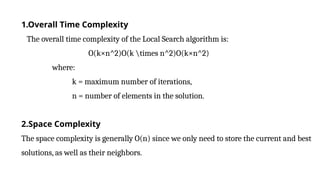
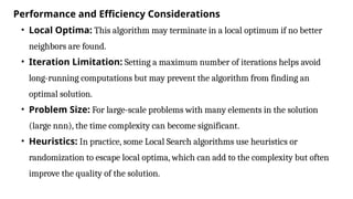
Local search algorithms are used to find approximate solutions for optimization problems by iteratively improving an initial solution through exploration of neighboring solutions. They include methods like hill climbing and simulated annealing, with a focus on performance affected by problem size and iteration limits. The algorithm's efficiency is defined by its time complexity of O(k×n^2) and is enhanced using techniques like multi-start local search.

1. Local
Search
Algorithm

2. What Are Local Search
Algorithms?
• Definition: Local search algorithms are used to find approximate
solutions for optimization problems.
• Goal: To iteratively improve an initial solution by exploring its
"neighborhood" and moving towards better solutions.
• Application: Common in combinatorial optimization, where
the search space is large and exact solutions are difficult.

3. Key Features
• Initial Solution: The starting point of the search.
• Neighboring Solutions: A set of nearby solutions
generated from the current one.
• Move to a Neighbor: Selecting a better solution from the
neighbors.
• Stopping Condition: When no further improvement is
possible, or the solution reaches an acceptable level of
quality.

4. Types of Local Search Algorithms
• Hill Climbing
• Simulated
Annealing
• Tabu Search
• Greedy Local Search

5. Workin
g
• Initialization: Start with an initial solution, which can be generated randomly or through
some heuristic method.
• Evaluation: Evaluate the quality of the initial solution using an objective function or a
fitness measure. This function quantifies how close the solution is to the desired outcome.
• Neighbor Generation: Generate a set of neighboring solutions by making minor changes
to the current solution. These changes are typically referred to as "moves."

6. • Selection: Choose one of the neighboring solutions based on a criterion, such as the
improvement in the objective function value. This step determines the direction in which
the search proceeds.
• Termination: Continue the process iteratively, moving to the selected neighboring
solution, and repeating steps 2 to 4 until a termination condition is met. This condition
could be a maximum number of iterations, reaching a predefined threshold, or finding a
satisfactory solution
Cont..,

7. Local_Search(initial_solution, max_iterations):
current_solution ← initial_solution
best_solution ← current_solution
iteration ← 0
while iteration < max_iterations do:
neighbor ← Get_Best_Neighbor(current_solution)
if neighbor is better than current_solution:
current_solution ← neighbor
if neighbor is better than best_solution:
best_solution ← neighbor
else:
break // No better neighbor found, stop search
iteration ← iteration + 1
return best_solution
Algorithm
:

8. 1.Overall Time Complexity
The overall time complexity of the Local Search algorithm is:
O(k×n^2)O(k times n^2)O(k×n^2)
where:
k = maximum number of iterations,
n = number of elements in the solution.
2.Space Complexity
The space complexity is generally O(n) since we only need to store the current and best
solutions, as well as their neighbors.

9. Performance and Efficiency Considerations
• Local Optima: This algorithm may terminate in a local optimum if no better
neighbors are found.
• Iteration Limitation: Setting a maximum number of iterations helps avoid
long-running computations but may prevent the algorithm from finding an
optimal solution.
• Problem Size: For large-scale problems with many elements in the solution
(large nnn), the time complexity can become significant.
• Heuristics: In practice, some Local Search algorithms use heuristics or
randomization to escape local optima, which can add to the complexity but often
improve the quality of the solution.

10. • Local Search’s efficiency depends on the size of the problem (n) and the maximum
iterations allowed (k).
• The time complexity of O(k×n^2)O(k times n^2)O(k×n^2) shows that the algorithm
is efficient for smaller values of n or k but may become slow for large-scale
optimization problems.
• To improve the performance, techniques like multi-start local search (restarting from
different initial solutions) or heuristic methods (like Simulated Annealing or Tabu
Search) are often used in conjunction with Local Search.
Conclusion

11. Thanks
!